Off Line Quality Control in Bioproducts Processing: A Case Study in Greece

(1)

http://dx.doi.org/10.4236/ojs.2016.62020

Off-Line Quality Control in Bioproducts

Processing: A Case Study in Greece

Ioannis S. Triantafyllou

Department of Statistics and Insurance Science, University of Piraeus, Piraeus, Greece

Received 22 January 2016; accepted 18 April 2016; published 21 April 2016

This work is licensed under the Creative Commons Attribution International License (CC BY). http://creativecommons.org/licenses/by/4.0/

Abstract

In the present article we study the production of grape molasses. Data drawn from a specified bi-olaboratory, are properly analyzed in order to detect factors that affect significantly the Brix value and the volatile acidity of the final product. The ground that is used for planting and a variety of grapes have been taken into account. Off-line statistical quality control techniques have been em-ployed and the outcomes are displayed and discussed in detail.

Keywords

Grape Molasses, Bioproduct, Statistical Quality Control, Analysis of Variance

1. Introduction

Statistical quality control is a useful tool for ensuring that the quality characteristics of a product are at the no-minal or required levels and consists of a set of statistical methods for analyzing data. The overall group of the abovementioned techniques is divided into three main subsets, namely Design of Experiments (off-line techniques), Statistical Process Control (on-line monitoring) and Acceptance Sampling. For more details for the on- line monitoring of a productive process, the interested reader is referred to the early work [1] or to the more re-cent contributions of [2]-[5] or the books [6] and [7].

The present study focuses on the quality control of the production process of a biological product called grape molasses (or petimezi). This product is made by 100% biological grapes, without using any pesticides. Grape molasses has attracted some research interest in the last decade; for example one may refer to publications

(2)

petimezi is undiluted must, produced by boiled-down grape juice and it is rich in energy, iron and calcium. It is used self-same in cooking and pastry and constitutes an ersatz of sugar or honey. Since bioproducts are not much prevalent in Greece, it is of some research interest to give space to statistical studies that aim at the devel-opment of the Greek biological cultivation.

The present study focuses on the quality improvement of the final bioproduct by examining the effect of some qualitative characteristics to volatile acidity and Brix value of grape molasses. In Section 2, the statistical me-thodology that is applied throughout this study, is presented in some detail. More specifically, statistical quality control techniques and analysis of variance models are applied in order to investigate the quality of petimezi produced in the aforementioned laboratory. Factors such as the variety of grapes used or the kind of ground, where the cultivation has taken place, are considered and properly analyzed. The results of the analysis are pre-sented comprehensively in Section 3. Finally, Section 4 offers a summary of the conclusions extracted by statis-tical analysis and formulizes several suggestions that may lead to the quality improvement of the final product.

2. Methods

The study used data drawn during 2014 from the biolaboratory of the company “KARAGGELIS OE”. The re-sponse variables of the study are determined to be the Brix value and the volatile acidity of must and grape mo-lasses. Each of the aforementioned quantitative characteristics has been examined whether is strongly affected or not, by a set of qualitative factors such as the variety of grapes and the type of ground that have been used. Analysis of Variance models have been appropriately applied in order to shed light on the above subject. Fur-thermore, multiple comparisons among the available levels of each factor have been presented by using the Tu-key method. In addition, off-line quality control tools, such as Taguchi measures (see, e.g. [11]), or linear re-gression analysis have been applied in order to detect effectively those factors that control noise or target of the bioproducts processing.

3. Main Results

In this section, we shall employ appropriate statistical methodologies in order to analyze data collected from the ad hoc laboratory, mentioned in the previous section, where the bioproduct of grape molasses is brought forth. The main objective of the present data analysis is to detect qualitative factors that have important effect on the volatile acidity and Brix value of the bioproduct of petimezi. Moreover, methods of Statistical Quality Control are also applied in order to determine the appropriate measures of noise and target, while based on the proposed measures, we shall appraise those factors that contribute significantly to the variability and central tendency of the volatile acidity and Brix value of the final bioproduct.

The laboratory that is under our study, is located in continental Greece and more specifically in Peloponnese. The grape molasses that is turned out, is affected basically by two factors; the first one refers to the variety of grape that is planted (factor A, hereafter). The second factor is associated with the ground, where the cultivation is taken place (factor B, hereafter). In the line of grape molasses production, the tilled ground is a three-level factor (lowland, semi-mountain, mountain), while the variety of grape is characterized by five levels (Merlot, Agiorgitiko, Camborne, Corinthian, Phocean).

Data have been appropriately collected so that at least two repetitions for each of the fifteen possible therapies have been accomplished. The number of available repetitions for each therapy, assures that the variance within each therapy could be estimated (see, e.g. [12]).

Let us next denote by Y1, Y2 the Brix value of must and grape molasses respectively, while Y3, Y4 express the volatile acidity of each of them. The main results section is organized as follows. At the beginning, the Brix value of must (Y1-value) is under investigation. Analysis of variance (ANOVA) is carried out and the corres-ponding results are discussed in detail. In addition, using the appropriate measures, we detect significant factors that control the variability and the central tendency of Y1-value in the bioproductive process. Similar outcomes are also reported for the rest characteristics, e.g. the Brix value of grape molasses and the volatile acidity of must and petimezi.

We next apply ANOVA model in order to divide the total variability of Brix characteristic of must, into two parts; the first one is related to measurable and manageable variables (see, e.g. factor A or B), while the second one comes unmanageable or from random causes.

(3)

and at least two repetitions for each therapy. The full-factorial model that has been initially applied is given as follows

( )

1, 2, 3, 4, 5 , 1, 2, 3

1, 2,

ijk i j ij ijk

i

y a a e j

k

µ

β

=   = + + + + _ =  =   (1)

where μ is the mean of Y1-values, ai (βj) represents the main effect of the i-th (j-th) level of factor A (B),

( )

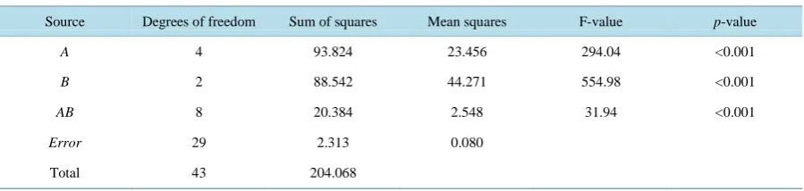
aβ _ij indicates the interaction term between the i-th level of factor A and the j-th level of factor B, while eijk is the cor-responding estimated residual. The results are summarized in Table 1.

One may easily conclude that the main effects of factors A, B and the respective interaction term are all sig-nificant at significance level 5% (p < 0.001). In words, the Brix value of must that accompanies the bioproduct, is strongly affected by the specific variety of grapes that is planted and the kind of ground that is used. In addi-tion, the effect of variety of grapes on Brix value of must, is strongly differentiated by the choice of the ground and reversely. In order to shed light on the pairwise comparisons between the mean values of different levels of each factor, the following Tukey simultaneous 95% confidence intervals are constructed.

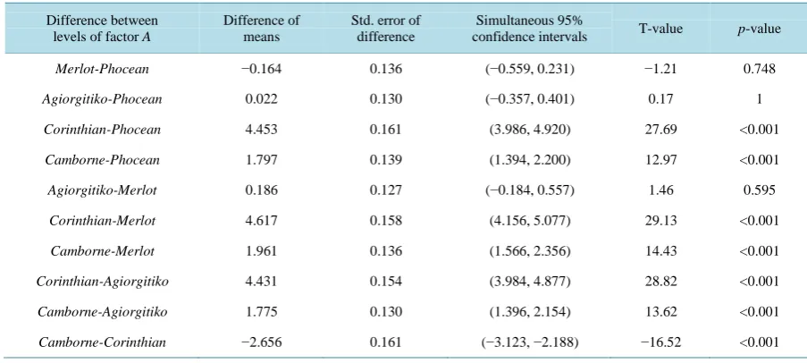
Since the larger is the Brix value, the better is the must, we may readily deduce at significance level 5% (see

Table 2) that

• Camborne variety gains the better of Phocean, Merlot and Agiorgitiko variety.

• Corinthian variety gains the better of Phocean, Merlot, Camborne and Agiorgitiko variety. In a similar way, we may conclude that at significance level 5% (see Table 3),

• mountain ground gains the better of lowland and semi-mountain ground. • semi-mountain ground gains the better of lowland ground.

In the sequel, we shall investigate whether factors A and B can be characterized as control factors of noise or control factors of target of Y1-values. According to Taguchi guidelines (see, e.g. [11] or [13]), the appropriate target measure is the average Brix value of must, while for the noise of the production, since the Brix value fol-lows the rule “the larger the better”, the proposed measure, named theta, is given as follows

2 10

1

10 log y

n

θ_{= −}  − 

 



∑

. (2)

Applying the appropriate ANOVA models for the aforementioned measures, the results are recapitulated in

Table 4 and Table 5.

Based on the above tables, we deduce that both factors A and B are characterized as control factors of noise and control factors of target. In order to bring out this confounding, an alternative measure for noise production should be used. More specifically, the proposed measure is given as follows (see, e.g. [13])

2 10 10 log b y m s   = _ _

  , (3)

[image:3.595.89.539.615.722.2]

where y, s is the sample mean and standard deviation of responses respectively, while the parameter b is re-lated to the possible existence of a functional connection between the population mean (μ) and standard devia-tion (σ). In other words, if a relation of the form σ=kµβ can be statistically affirmed, then the parameter b of

Table 1.ANOVA model: Brix value of must versus ground and variety.

Source Degrees of freedom Sum of squares Mean squares F-value p-value

A 4 93.824 23.456 294.04 <0.001

B 2 88.542 44.271 554.98 <0.001

AB 8 20.384 2.548 31.94 <0.001

Error 29 2.313 0.080

(4)

[image:4.595.85.537.100.303.2]

Table 2.Tukey pairwise comparisons: Brix value of must in terms of grapes variety.

Difference between

levels of factor A

Difference of means

Std. error of difference

Simultaneous 95%

confidence intervals T-value p-value

Merlot-Phocean −0.164 0.136 (−0.559, 0.231) −1.21 0.748

Agiorgitiko-Phocean 0.022 0.130 (−0.357, 0.401) 0.17 1

Corinthian-Phocean 4.453 0.161 (3.986, 4.920) 27.69 <0.001

Camborne-Phocean 1.797 0.139 (1.394, 2.200) 12.97 <0.001

Agiorgitiko-Merlot 0.186 0.127 (−0.184, 0.557) 1.46 0.595

Corinthian-Merlot 4.617 0.158 (4.156, 5.077) 29.13 <0.001

Camborne-Merlot 1.961 0.136 (1.566, 2.356) 14.43 <0.001

Corinthian-Agiorgitiko 4.431 0.154 (3.984, 4.877) 28.82 <0.001

Camborne-Agiorgitiko 1.775 0.130 (1.396, 2.154) 13.62 <0.001

Camborne-Corinthian −2.656 0.161 (−3.123, −2.188) −16.52 <0.001

Table 3. Tukey pairwise comparisons: Brix value of must in terms of ground.

Difference between

levels of factor B

Difference of means

Std. Error of Difference

Simultaneous 95%

Confidence Intervals T-value p-value

Semi-mountain-Lowland 1.891 0.104 (1.634, 2.149) 18.12 <0.001

Mountain-Lowland 3.825 0.115 (3.540, 4.110) 33.17 <0.001

[image:4.595.87.541.429.637.2]

Mountain-Semi-mountain 1.933 0.114 (1.652, 2.215) 16.94 <0.001

Table 4.ANOVA model: Theta measure of Brix value of must versus ground and variety.

A 4 5.0522 1.2631 11.29 0.002

B 2 4.3907 2.1953 19.62 0.001

Error 8 0.8950 0.1119

Total 14

Table 5.ANOVA model: Target measure of Brix value of must versus ground and variety.

A 4 40.375 10.094 12.08 0.002

B 2 32.694 16.347 19.57 0.001

Error 8 6.682 0.835

Total 14

the above formula should be estimated via an appropriate regression analysis. Otherwise, the parameter b shall be replaced by zero. If we denote by y_i, si the mean and standard deviation of responses in the i-th trial, the outcomes of the regression analysis between them, are summarized in Table 6.

(5)

analysis of this measure revealed that neither variety of grapes nor the ground could be characterized as control factors of noise anymore. Therefore, our final deduction is that we should adjust properly the factors A and B in order to control the target value of Brix measurements of must.

Employing analogous arguments, one may draw similar conclusions for the remaining quantitative responses of the experiment, such as the Brix value of grape molasses (Y2-value) or the volatile acidity of must (Y3-value) and petimezi (Y4-value). As far it concerns with the Brix value of grape molasses, the ANOVA disclosed that both factors A and B affect significantly the response of each trial (p < 0.001, see Table 7).

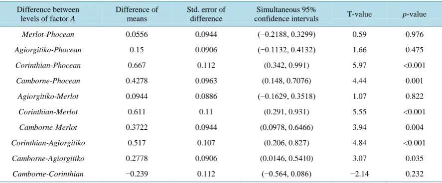
However, there seems to be a negligible interaction between them (p = 0.093). Taking a look at the pairwise comparisons between levels of factor A (see Table 8), we observe the following

• Camborne variety gains the better of Phocean, Agiorgitiko and Merlot variety. • Corinthian variety gains the better of Phocean, Merlot and Agiorgitiko variety.

In a similar way, we may conclude that at significance level 5% mountain ground gains the better of lowland and semi-mountain ground (see Table 9).

[image:5.595.87.539.317.387.2]

According to Taguchi guidelines, the appropriate target measure is the average Brix value of petimezi, while for the noise of production is given in Equation (3). Table 10 andTable 11 reveal that factors A and B can be characterized only as controllers of target value while noise of the production seems not to be controlled by them.

Table 6. Regression model for Brix value of must: Logarithm of standard deviation versus logarithm of mean.

Logarithm of mean 1 0.45518 0.45518 6.92 0.021

Error 13 0.85485 0.06576

[image:5.595.97.539.414.509.2]

Regression equation Logsi= −6.32+4.18Logyi

Table 7.ANOVA model: Brix value of grape molasses versus ground and variety.

A 4 2.036 0.5090 13.22 <0.001

B 2 1.034 0.5170 13.43 <0.001

AB 8 0.5946 0.0743 1.93 0.093

Error 29 1.1167 0.0385

Total 43 5.0480

Table 8.Tukey pairwise comparisons: Brix value of grape molasses in terms of grapes variety.

Difference between

levels of factor A

Difference of means

Simultaneous 95%

Merlot-Phocean 0.0556 0.0944 (−0.2188, 0.3299) 0.59 0.976

Agiorgitiko-Phocean 0.15 0.0906 (−0.1132, 0.4132) 1.66 0.475

Corinthian-Phocean 0.667 0.112 (0.342, 0.991) 5.97 <0.001

Camborne-Phocean 0.4278 0.0963 (0.148, 0.7076) 4.44 0.001

Agiorgitiko-Merlot 0.0944 0.0886 (−0.1629, 0.3518) 1.07 0.822

Corinthian-Merlot 0.611 0.11 (0.291, 0.931) 5.55 <0.001

Camborne-Merlot 0.3722 0.0944 (0.0978, 0.6466) 3.94 0.004

Corinthian-Agiorgitiko 0.517 0.107 (0.206, 0.827) 4.84 <0.001

Camborne-Agiorgitiko 0.2778 0.0906 (0.0146, 0.5410) 3.07 0.035

[image:5.595.94.538.537.721.2]

(6)

Table 9.Tukey pairwise comparisons: Brix value of grape molasses in terms of ground.

Difference between

levels of factor A

Difference of means

Simultaneous 95%

Semi-mountain-Lowland 0.12 0.0725 (−0.059, 0.299) 1.65 0.24

Mountain-Lowland 0.41 0.0801 (0.2123, 0.6077) 5.12 <0.001

Mountain-Semi-mountain 0.29 0.0793 (0.0943, 0.4857) 3.66 0.003

Table 10.ANOVA model: Noise measure of Brix value of petimezi versus ground and variety.

A 4 11.172 2.793 2.23 0.156

B 2 0.424 0.212 0.17 0.847

Error 8 10.038 1.255

Total 14 21.633

Table 11.ANOVA model: Target measure of Brix value of petimezi versus ground and variety.

A 4 0.8184 0.2046 8.79 0.005

B 2 0.3841 0.19206 8.25 0.011

Error 8 0.1863 0.02328

Total 14 1.3888

On the other hand, the volatile acidity of must (Y3-values) is not affected by the ground that has been used for planting, since the corresponding observed significance is equal to 0.979 (see Table 12).

Grapes variety seems to affect significantly the response Y3 (p = 0.002) of the experiment. Based on multiple comparisons between levels of factor A displayed in Table 13, one may readily deduce the following

• Phocean grapes variety gains the better of Agiorgitiko and Camborne grapes variety. • Corinthian grapes variety gains the better of Camborne and Agiorgitiko grapes variety.

According to Taguchi guidelines, the appropriate target measure is the average volatile acidity of must, while for the noise of measurements, based on the rule “the smaller the better”, is given as

2 10

1

10 log .

h y

n

 

= − _ _



∑

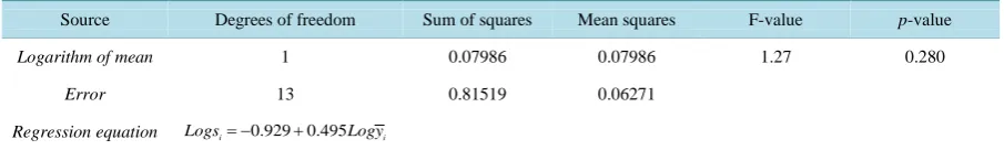
 (4) The analysis of the above measures, leads to the conclusion that grapes variety seems to control both target and noise (see Table 14 and Table 15).

Following similar methodology as before, we construct an alternative measure for noise (see Equation (3)), where the parameter b has been proved non-significant (p = 0.28, Table 16).

Therefore the proposed measure m is given as

10 20 log .

m= − s (5)

Based on the above measure, factors A and B do not seem to control noise, while factor A remains as the one that controls central tendency of the Y3 responses (see Table 17).

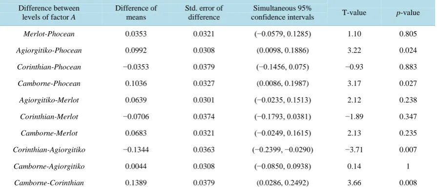
Finally, the volatile acidity of petimezi is not affected by the ground that has been used for planting, since the corresponding observed significance is equal to 0.958 (see Table 18).

(7)

[image:7.595.89.538.101.199.2]

Table 12.ANOVA model: Volatile acidity of must versus ground and variety.

A 4 0.127454 0.031864 5.54 0.002

B 2 0.000248 0.000124 0.02 0.979

AB 8 0.076828 0.009604 1.67 0.149

Error 29 0.166758 0.00575

[image:7.595.101.537.224.409.2]

Total 43 0.374891

Table 13.Tukey pairwise comparisons: Volatile acidity of must in terms of grapes variety.

Difference between

levels of factor A

Difference of means

Simultaneous 95%

Merlot-Phocean 0.0436 0.0365 (−0.0624, 0.1496) 1.2 0.754

Agiorgitiko-Phocean 0.1094 0.035 (0.0077, 0.2111) 3.13 0.030

Corinthian-Phocean −0.0381 0.0432 (−0.1635, 0.0874) −0.88 0.901

Corinthian-Merlot −0.0817 0.0425 (−0.2053, 0.042) −1.92 0.330

Camborne-Merlot 0.0681 0.0365 (−0.0380, 0.1741) 1.87 0.358

Corinthian-Agiorgitiko −0.1475 0.0413 (−0.2675, −0.0275) −3.57 0.010

Camborne-Agiorgitiko 0.0022 0.0350 (−0.0995, 0.1039) 0.06 1

[image:7.595.87.540.436.516.2]

Camborne-Corinthian 0.1497 0.0432 (0.0243, 0.2752) 3.47 0.013

Table 14.ANOVA model: Noise measure h of volatile acidity of must versus ground and variety.

A 4 50.462 12.6155 4.16 0.041

B 2 1.922 0.9610 0.32 0.737

Error 8 24.246 3.0308

Total 14 76.630

Table 15.ANOVA model: Target measure of volatile acidity of must versus ground and variety.

A 4 0.04584 0.01146 3.83 0.050

B 2 0.00036 0.00018 0.06 0.942

Error 8 0.02395 0.00299

Total 14 0.07015

Table 16.Regression model for volatile acidity of must: Logarithm of standard deviation versus logarithm of mean.

Error 13 0.81519 0.06271

[image:7.595.89.538.543.626.2] [image:7.595.87.540.652.720.2]

(8)

[image:8.595.88.537.101.185.2]

Table 17.ANOVA model: Noise measure m of volatile acidity of must versus ground and variety.

A 4 90.12 22.53 1.38 0.323

B 2 13.7.19 68.60 4.20 0.057

Error 8 130.70 16.34

[image:8.595.89.539.214.317.2]

Total 14 358.02

Table 18.ANOVA model: Volatile acidity of petimezi versus ground and variety.

A 4 0.108403 0.027101 6.10 0.001

B 2 0.000378 0.000189 0.04 0.958

AB 8 0.063741 0.007968 1.79 0.119

Error 29 0.128858 0.004443

Total 43 0.304173

Table 19.Tukey pairwise comparisons: Volatile acidity of petimezi in terms of grapes variety.

Difference between

levels of factor A

Difference of means

Simultaneous 95%

Merlot-Phocean 0.0353 0.0321 (−0.0579, 0.1285) 1.10 0.805

Agiorgitiko-Phocean 0.0992 0.0308 (0.0098, 0.1886) 3.22 0.024

Corinthian-Phocean −0.0353 0.0379 (−0.1456, 0.075) −0.93 0.883

Corinthian-Merlot −0.0706 0.0374 (−0.1793, 0.0381) −1.89 0.347

Camborne-Merlot 0.0683 0.0321 (−0.0249, 0.1615) 2.13 0.235

Corinthian-Agiorgitiko −0.1344 0.0363 (−0.2399, −0.0290) −3.71 0.007

Camborne-Agiorgitiko 0.0044 0.0308 (−0.0850, 0.0938) 0.14 1

Camborne-Corinthian 0.1389 0.0379 (0.0286, 0.2492) 3.66 0.008

• Phocean grapes variety gains the better of Agiorgitiko and Camborne grapes variety. • Corinthian grapes variety gains the better of Camborne and Agiorgitiko grapes variety.

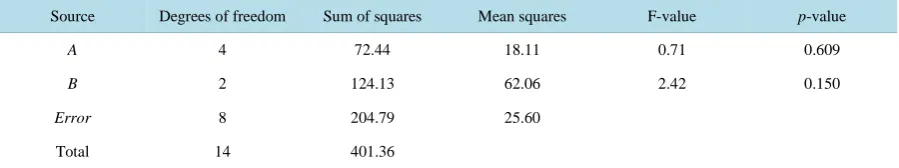
The analysis of measures proposed by Taguchi, leads to the conclusion that grapes variety seems to control both target and noise. Following similar methodology as before, we construct an alternative measure for noise (see Equation (3)), where the parameter b is non-significant (p = 0.354, Table 20).

Therefore the proposed measure takes on the form presented in Equation (5). Based on the aforementioned measure, there is no factor that seems to control noise, while factor A remains as the one that controls central tendency of the response Y4 (see Table 21).

4. Conclusion

[image:8.595.92.540.347.543.2]

(9)

[image:9.595.85.539.101.171.2]

Table 20.Regression model for volatile acidity of petimezi: Logarithm of standard deviation versus logarithm of mean.

Error 13 0.93693 0.07207

Regression equation Logsi= −1.019 0.424+ Logyi

Table 21.ANOVA model: Noise measure of volatile acidity of petimezi versus ground and variety.

A 4 72.44 18.11 0.71 0.609

B 2 124.13 62.06 2.42 0.150

Error 8 204.79 25.60

Total 14 401.36

of grapes that are planted and the ground where the cultivation is taken place, have been proved significant fac-tors for the quality of the final product. Corinthian and Camborne varieties of grapes seem to lead to the opti-mum result as far it concerns the Brix value of must and grape molasses, while Phocean and Corinthian varieties of grapes are the best choices in order to abate their volatile acidity. On the other hand, mountain ground has been proved as the one that is capable to optimize Brix value of must and grape molasses. It is of some interest for future research, to depict and analyze additional characteristics of grapes molasses in order to enhance the quality of the bioproductive process of it.

Acknowledgements

The author wish to thank the anonymous referees for their useful comments and suggestions which improved the presentation of the paper.

References

[1] Shewhart, W.A. (1926) Quality Control Charts. Bell System Technical Journal, 2, 593-603.

http://dx.doi.org/10.1002/j.1538-7305.1926.tb00125.x

[2] Balakrishnan, N., Triantafyllou, I.S. and Koutras, M.V. (2009) Nonparametric Control Charts Based on Runs and Wil-coxon-Type Rank-Sum Statistics. Journal of Statistical Planning and Inference, 139, 3177-3192.

http://dx.doi.org/10.1016/j.jspi.2009.02.013

[3] Balakrishnan, N., Triantafyllou, I.S. and Koutras, M.V. (2010) A Distribution-Free Control Chart Based on Order Sta-tistics. Communication in Statistics—Theory and Methods, 39, 3652-3677.

http://dx.doi.org/10.1080/03610920903324858

[4] Chakraborti, S. (2011) Nonparametric (Distribution-Free) Quality Control Charts. Encyclopedia of Statistical Sciences, 1-27. http://dx.doi.org/10.1002/0471667196.ess7150

[5] Chowdhury, S., Mukherjee, A. and Chakraborti, S. (2015) Distribution-Free Phase II CUSUM Control Chart for Joint Monitoring of Location and Scale. Quality and Reliability Engineering International, 31, 135-151.

http://dx.doi.org/10.1002/qre.1677

[6] Gibbons, J.D. and Chakraborti, S. (2010) Nonparametric Statistical Inference. 5th Edition, Marcel Dekker, New York.

[7] Balakrishnan, N. and Ng, H.K.T. (2006) Precedence-Type Tests and Applications. John Wiley & Sons, Hoboken.

http://dx.doi.org/10.1002/0470037849

[8] Toker, O.S. and Dogan, M. (2013) Effect of Temperature and Starch Concentration on the Creep/Recovery Behavior of the Grape Molasses: Modelling with ANN, ANFIS and Response Surface Methodology. European Food Research and Technology, 236, 1049-1061. http://dx.doi.org/10.1007/s00217-013-1959-0

[image:9.595.89.539.199.283.2]

(10)

[10] Erdogrul, O. (2008) Pesticide Residues in Liquid Pekmez (Grape Molasses). Environmental Monitoring and Assess-ment, 144, 323-328. http://dx.doi.org/10.1007/s10661-007-9995-5

[11] Taguchi, G. (1986) Introduction to Quality Engineering: Designing Quality into Products and Processes. Asian Produc-tivity Organization, Tokyo.

[12] Montgomery, D.C. (2012) Design and Analysis of Experiments. 8th Edition, John Wiley & Sons, New York. [13] Logothetis, N. and Wynn, H.P. (1989) Quality through Design: Experimental Design, Off-Line Quality Control and