Munich Personal RePEc Archive
Simulation Based Estimation of Discrete
Sequential Move Games of Perfect
Information
Wang, Yafeng and Graham, Brett
Wang Yanan Institute for Studies in Economics, Xiamen University
8 July 2010
Online at
https://mpra.ub.uni-muenchen.de/69281/
Simulation Based Estimation of Discrete Sequential
Move Games of Perfect Information
∗
Yafeng Wang
and
Brett Graham
†Wang Yanan Institute for Studies in Economics (WISE) Xiamen University
Abstract
We propose simulation based estimation for discrete sequential move games of perfect information which relies on the simulated moments and importance sampling. We use importance sampling techniques not only to reduce computational burden and simulation error, but also to overcome non-smoothness problems. The model is identified with only weak scale and location normalizations, monte Carlo evidence demonstrates that the estimator can perform well in moderately-sized samples.
Keywords: Game-Theoretic Econometric Models; Sequential-Move Game; Method of Simulated Moments; Importance Sampling; Conditional Moment Restrictions.
JEL Classification Numbers: C01, C13, C35, C51, C72.
∗Preliminary version, comments are welcome.
†We would like to thank participants at Chinese Economists Society 2010 Annual Conference for
1
INTRODUCTION
Nash equilibrium is one of the cornerstones of modern economic theory, with substantive application in all major fields in economics, particularly industrial organization. It is the benchmark theoretical model for analyzing strategic interactions among a handful of players. Given the importance of gaming in economic theory, the empirical analysis of games has been the focus of a recent literature in econometrics and industrial organization, such as Tamer (2003), Berry & Tamer (2007), Aguirregabiria & Mira (2007), Aradillas-Lopez (2007, 2008), Ciliberto & Tamer (2009), Bajari, Hong, Krainer & Nekipelov (2010) and Bajari, Hong & Ryan (2010) (hereafter BHR).
(Geweke (1989, 1991), Hajivassiliou & McFadden (1998) and Keane (1990, 1994)), which he called as ”sequential GHK”. The estimator provided by Maruyama (2009) essentially is a maximum simulated likelihood (MSL) estimator, As is well known, MSL is biased for any fixed number of simulations, in order to obtain √T consistent estimators, one needs to increase the number of draws N S so that N S√
T → ∞. Wang & Graham (2009) provides
a generalized maximum entropy (GME) estimator for this class of games which avoids the usual multidimensional integrals by using the data constraints instead of the mo-ment constraints, they reformulate the estimation problem as a mixed-integer nonlinear optimization problem since there are logical connections between endogenous variables among the equilibrium conditions, although the computational burden is acceptable for most applications, it is hard to construct large sample properties for this GME estimator, since essentially it is a nonsmooth estimation1
.
In this paper, we propose a simulation based estimator for discrete sequential move games of perfect information which relies on the simulated moments and importance sampling. As noted by Maruyama (2009), the estimation of sequential games has some distinctive features and advantages over simultaneous games, the most advantage is that perfect information sequential games can utilize the notion of subgame perfection, which guarantees the existence of unique equilibria, however, in simultaneous games of complete information, the existence of multiple equilibria is sometimes considered problematic or at least an issue to deal with (see for example, Ciliberto & Tamer, 2007; BHR, 2010).
The moment conditions implied by the model equilibrium conditions in discrete se-quential move games of perfect information contain multidimensional integrals, in princi-ple, one can use straightforward Monte Carlo simulations to get unbiased estimators for such multidimensional integrals, but there are several problems that can arise with estima-tors based on such simulations. First, there are discrete parts of the model, the objective
1
function in the estimation procedure is typically discontinuous in the parameter vector, making it hard to minimize (maximize) correctly; Second, the straightforward Monte Carlo simulations need to solve the game numerous times, typically once for every draw, for every observation, for every parameter vector that is ever evaluated in an optimization procedure. If we have T observations, performs N S simulation draws, and optimization requires R function evaluations, estimation requires solving the modelN S∗T ∗R times, this can be computationally time consuming sinceRcan be quite large. In spirit of Acker-berg (2009) and BHR (2010), we make use of importance sampling to overcome both of the problems, by finding the right change of variables to do the importance sampling over, the simulated approximation of the multidimensional integral (expectation) will generally be continuous in the parameter vector, and also one reduce the times of solving the game fromN S∗T∗R toN S∗T.2
In order to make use of importance sampling, it is important to make sure that the tails of the importance density are not too thin in a neighborhood of the parameter that minimizes (maximizes) the objective function in the estimation procedure, the GME estimator proposed by Wang & Graham (2009) can be used to con-struct the importance density, or one can make use of the MSL estimator proposed by Maruyama (2009). Based on such simulated moments, we propose two estimators for the discrete sequential move games of perfect information, one is the method of simulated moments (MSM), which is same as the usual GMM estimation but use the simulated mo-ments instead of the true momo-ments. Given that the equilibrium conditions are conditional moment restrictions, same as the GMM estimation, MSM estimation may induce incon-sistent estimates due to the number of arbitrarily chosen instruments is finite, we make use of the always consistent estimation procedure that is directly based on the definition of the conditional moments proposed by Dominguez & Lobato (2004). Our monte Carlo experiments show that the always consistent estimator performs better than the MSM
2
estimator, especially in the small sample size.
The paper is organized as follows. In section 2 we outline the general discrete sequential-move games to be estimated and formulate its equilibrium conditions, the as-sumptions for the identification and estimation also are presented. Section 3 formalizes our simulation and estimation approach. Monte Carlo simulations are conducted in sec-tion 4. Secsec-tion 5 concludes, and provides limitasec-tions and future work.
2
THE MODEL
We use the strategic environment of BHR (2010) to develop our estimation method. In the model, there are T independent repetitions of a sequential move game of perfect information (extensive form game). In each game there are i = 1, ..., Nt players, each
with the finite set of actionsAit. DefineAt=×iAit and letat= (a1t, ..., ait, ...aN t) denote
a generic element of At. Without loss of generality, the order of subscripts for players
(1, ..., Nt) also represents the decision order of the sequential move game in each repetition,
that means player 1 makes decision first and playerNtat the end. Playeri’s von
Neumann-Morgenstern (vNM) utility is a map uit : At → R, where R is the real line. Since we
study the sequential move game, the corresponding equilibrium concept is the subgame perfect equilibria (SPE), this can be achieved when every player expects no gain from individually deviating from its equilibrium strategy in its every subgame, the standard technique for solving the SPE is backward induction, furthermore, the finite sequential move game of perfect information where there is no player is indifference between any two outcomes has a unique SPE. We will sometimes drop the subscript t for simplicity when no ambiguity would arise.
The vNM utility of player i is assumed to be:
In Equation (1), player i’s vNM utility from action a is the sum of two terms. The first term Πi(x, a;θ) is a function which depends ona, the vector of actions taken by all of the
players, covariatesx, the players’ characteristics and some other variables which influence the utility, and parametersθ, covariatesxare observed to the econometrician. The second term isϵi(a), a random preference shock which reflects the information about utility that
is common knowledge to the players but not observed by the econometrician. Unlike Maruyama (2009), here the preference shocks depend on the entire vector of actionsa, not just the actions taken by playeri. As argued by BHR (2010), this is a more general setting and seems straightforward within the game framework, think about a simple entry game, the unobserved information of one player to econometrician may be different not only among players but also action vector dependent3
. ϵi(a) are assumed to be independent,
let ϵi denote the vector of the individual ϵi(a) and ϵi denote the vector of all the shocks.
we will discuss more about the structure ofϵi in the model assumptions.
As noted above, the equilibrium concept corresponding to the sequential move game of perfect information, SPE, is a equilibrium strategy profile which means that every player expects no gain from individually deviating from its equilibrium in every subgame. A strategy of player i ∈ N is a function that assigns an action in Ai to each nonterminal
history, a player’s deviation form equilibrium holding other’s decisions fixed does not mean that all the others make the same decision, it means the others follow the same strategy. But what can be observed is only the equilibrium actions (i.e., equilibrium outcome). Thus, for deriving the equilibrium conditions in our econometric model, we should make the others’ action profile when one player deviating as endogenous variable. Formally, an SPE action profile,aSP E = (aSP E
1 , ...aSP Ei , ...aSP EN ), is any solution for the decisions of the
3
players that satisfies:
ui(aSP Ei , a SP E
−i , x, ϵi;θ)−ui(ai, aSP E<i , a∗>i(a SP E
<i , ai), x, ϵi;θ)≥0 (2)
for all i= 1, ..., N and all ai ̸=aSP Ei .
where a∗
>i(aSP E<i , ai) is a SPE action profile for the subgame that starts from player i+ 1
given the decisions of the preceding players,a≤i. This equilibrium conditions are defined
recursively and the solution can be easily calculated by the backward induction for any given parameters θ, observed covariates, x, and unobservable shocks ϵ. Kuhn’s theorem ensures the existence of solutions of the inequality system (2) but makes no claim of uniqueness, thus we can conclude that every finite sequential move game of perfect infor-mation has a SPE. As noted by Berry & Tamer(2007), dealing with multiple equilibria complicate the identification problem, fortunately, a modified version of Kuhn’s theorem ensures the uniqueness of equilibria of finite sequential move games of perfect information, which is presented in theorem 1.
Theorem 1 Every finite sequential move game with perfect information in which no
player is indifference between any two outcomes has a unique subgame perfect equilibrium.
Proof. See Osborne & Rubinstein (1994).
Obviously, the indifference case can be ignored in our econometric model since we work with continuous latent payoffs (ϵi(a) has an atomless distribution). Given such
structure of the discrete choice sequential move game, our task is to estimate and draw an inference about the parameters of payoff functions, θ, with the observation of action profileao, some covariates which have effect on the payoffs, x, and an exogenous decision
2.1
Assumptions
Assumption 1 (Exogenous Decision Order) The decision order of agents in the
se-quential move game is exogenous.
Although the exact decision order of agents is rarely observed, we can estimate se-quential move games by imposing different decision order assumptions, this restriction only excludes the endogenous decision order which may alter the uniqueness of the game structure.
Assumption 2 (Scale and Location Normalizations) The payoff of one action for
each player is fixed at a known constant.
As argued by BHR (2010), this restriction is similar to the argument that we can normalize the mean utility from the outside good equal to a constant, usually zero, in a standard discrete choice model. One clearly find that from the equilibrium condition (2) that adding a constant to all deterministic payoffs does not perturb the set of equilib-ria, so a location normalization is necessary. A scale normalization is also necessary, as multiplying all deterministic payoffs by a positive constant does not alter the SPE. This restriction is subsumed in the following assumption about the distribution of the error terms.
Assumption 3 (Regularity Conditions of Random Shocks) The joint distribution
of ϵ= (ϵi(a)), G(ϵ|β) is independent and known to all agents and the
econometri-cian.
3
ESTIMATION
Next, we propose computationally efficient simulation based estimators for θ and β, the parameters governing agents’ deterministic payoffs and the error terms’ distribution, given the observations of a sequence (at, xt) of action profiles and covariates. To form the
estimation framework, enumerate the elements of A from k = {1, ...,#A}. Denote the observation at tth repetition of the game with y
t and
yt=
I(at= 1)
.
I(at =k)
.
I(at = #A)
=f(xt, ϵt, θ0) (3)
where I(·) is the usual indicator function, f(xt, ϵt, θ) is an algorithm which solves the
game for any given xt, ϵt and θ, obviously, it is corresponding to the model equilibrium
conditions (2). Denote the probability that a specific action profilek is played implied by the model as P(k|xt;θ) and collect them into a vector P(a|xt;θ), where
P(a|xt;θ, β) =E[f(xt, ϵt, θ)|xt] =
∫
f(xt, ϵt, θ)dG(ϵ, β) (4)
At the true parameters of the data-generating process the predicted probability of each action equals its empirical probability of each actionk:
E[(yt−P(a|xt;θ, β))|xt] = 0 atθ =θ0, β =β0 (5)
1 conditional moment restrictions. Obviously, the expectation of any function w(xt)
of the conditioning variables multiplied by the difference between yt and the predicted
probabilities is identically zero at the true parameters, i.e.
E[w(xt)∗(yt−P(a|xt;θ, β))] =0 atθ =θ0, β =β0 (6)
In principle, the value ofθ and β, say ˆθ and ˆβ, that set the sample analog of this moment
GT(θ, β) =
1
T
∑
t
[w(xt)∗(yt−P(a|xt;θ, β))]
equal to zero or as close as possible to zero is a consistent estimator of θ0 and β0.
Un-der appropriate regularity conditions, one obtains asymptotic normality of the estimators (Hansen, 1982), and as the number of moments used increases, one can approach asymp-totic efficiency by the right choice of instruments (i.e. thew function).
To make use of such GMM estimation, we should overcome some obstacles, the first obstacle is that the predicted probabilitiesP(a|xt;θ, β) which defined by (4) is not easily
computable, since it involves a multidimensional integral, thus simulation enters the pic-ture. As can be found below, a straightforward Monte Carlo procedure is not practical due to the computational burden and discreteness in f(xt, ϵt, θ), we make use of importance
sampling to overcome such problems.
3.1
Simulation
The straightforward way of simulating
P(a|xt;θ, β) =E[f(xt, ϵt, θ)|xt] =
∫
is by averagingf(xt, ϵt, θ) over a set ofN Srandom draws (ϵ1, ..., ϵN S) from the distribution
of ϵt, G(ϵ|β), i.e.
˜
P(a|xt;θ, β) =
1
N S
∑
ns
f(xt, ϵt, θ) (7)
˜
P(a|xt;θ, β) is trivially an unbiased simulator of the true expectation P(a|xt;θ, β) =
E[f(xt, ϵt, θ)|xt]. McFadden (1989) and Pakes & Pollard (1989) prove statistical properties
of the MSM estimator that set the simulated moment:
˜
GT(θ, β) =
1
T
∑
t
[w(xt)∗(yt−P˜(a|xt;θ, β))]
= 1
T
∑
t
[w(xt)∗(yt−
1
N S
∑
ns
f(xt, ϵt, θ))] (8)
as close as possible to zero. The most important of these statistical properties is the fact that these estimators are typically consistent for finite N S. The intuition behind this is that simulation error averages out over observations as T → ∞. This consistency property gives the estimator an advantage over alternative estimation approaches such as maximum simulated likelihood (MSL), which typically is not consistent for a finite number of simulation draws. Another nice property of these estimators is that the extra variance imparted on the estimates due to the simulation is relatively small, asymptotically it is 1/N S. As noted above, an important obstacle of making use of MSM estimation procedure in our sequential game estimation is that f(xt, ϵt, θ) typically is not continuous in θ,
since the algorithm for solving the discrete sequential move game of perfect information essentially is a combination of several indicator functions, which is not continuous in θ. The discreteness in f(xt, ϵt, θ) will generate the discreteness in ˜P(a|xt;θ, β), as can be
found via a simple entry game conducted in example 1. Thus the simulated moments, ˜
GT(θ, β), will tend not to be continuous in θ, typically having both flats and jumps.
This can be very problematic in the numeric minimization of ˜GT(θ, β), derivative based
Example 1 To illustrate the discreteness problem, consider a simple two-firm sequential
entry game, where firm 1 moves first. Each firm has the following profit function:
ui(x, a, ϵi;θ) = 1(ai = 1){xiθ1 +N(a)θ2+ϵi(a)}
where ai ∈ {0,1} is firm i’s action, N(a) is the number of entrants for a action profile a.
Function f maps (x, ϵ, θ) into the market structure (outcome)y,
y=
I(0,0)
I(0,1)
I(1,0)
I(1,1)
=f(x, ϵ, θ)
For exposition we focus on the 2nd element of y, we can write this out explicitly as:
y2 =I(0,1) =I
[0> x1θ1+θ2+ϵ1(1,0) ∩ 0> x2θ1+ 2θ2+ϵ2(1,1)]
∪
[0> x1θ1+ 2θ2+ϵ1(1,1) ∩ 0≤x2θ1+ 2θ2+ϵ2(1,1)]
∩
x2θ1 +θ2+ϵ2(0,1)≥0
Obviously, function f is not continuos in θ. The straightforward simulator
˜
P((0,1)|xt;θ, β) =
1 N S ∑ ns I
[0> x1θ1+θ2 +ϵ1,ns(1,0) ∩ 0> x2θ1+ 2θ2+ϵ2,ns(1,1)]
∪
[0> x1θ1+ 2θ2+ϵ1,ns(1,1) ∩ 0≤x2θ1+ 2θ2+ϵ2,ns(1,1)]
∩
x2θ1+θ2+ϵ2,ns(0,1)≥0
is also not continuos in θ.
In spirit of Ackerberg (2009) and BHR (2010), we make use of importance sampling to reduce the non-smoothness problem4
. Importance sampling is most noted for its ability to reduce simulation error and computational burden, and was first used in game-theoretic models estimation by BHR (2010), who estimated norm form complete information games. First, we change the variable of integration in Equation (4) from ϵ to u. Let h(u|x, θ, β) denote the density of u, conditional on x, θ and β, and g(ϵi(a)|β) the density of ϵi(a).
Then the densityh(u|x, θ, β) is:
h(u|x, θ, β) = ∏
i
∏
a∈A
g(ui(a, x, ϵi;θ)−Πi(x, a;θ)|β) (9)
If we change the variable of integration in
P(a|xt;θ, β) =E[f(xt, ϵt, θ)|xt] =
∫
f(xt, ϵt, θ)dG(ϵ, β)
=
∫
f(xt, ϵt, θ)g(ϵ|β)dϵ
fromϵ to u, thenP(a|xt;θ, β) becomes:
P(a|xt;θ, β) =
∫
f(u)h(u|xt, θ, β)du (10)
In order to use importance sampling, introduce the importance density q(u), rewrite Equation (10) as:
P(a|xt;θ, β) =
∫
f(u)h(u|xt, θ, β)
q(u) q(u)du (11)
We can then simulate P(a|xt;θ, β) by draw random variables u1, ...uN S fromq(u) and
4
construct
ˆ
P(a|xt;θ, β) =
1
N S
N S
∑
ns=1
f(uns)
h(uns|xt, θ, β)
q(uns)
(12)
Note that
E[ ˆP(a|xt;θ, β)] =E[f(u)
h(u|xt, θ, β)
q(u) ] =
∫
f(u)h(u|xt, θ, β)
q(u) q(u)du =E[f(xt, ϵt, θ)|xt]
≡P(a|xt;θ, β)
So the importance sampling simulator ˆP(a|xt;θ, β) is an unbiased simulator for the true
expectation. The most important property of this simulator is that ˆP(a|xt;θ, β) will
generally be continuous in θ and β since it only depends on θ and β through h(u|xt, θ, β)
which is continuous in θ and β given that g(ϵ|β) is continuous, this can be revealed by using this simulator in the simple two-player entry game which conducted in Example 1.
Example 2 (Ex.1 Cont’) Consider the two-player entry game conducted in Example 1.
For exposition we also only focus on the 2nd element of y:
y2 =I(0,1) =I
[0> x1θ1+θ2+ϵ1(1,0) ∩ 0> x2θ1+ 2θ2+ϵ2(1,1)]
∪
[0> x1θ1+ 2θ2+ϵ1(1,1) ∩ 0≤x2θ1+ 2θ2+ϵ2(1,1)]
∩
x2θ1 +θ2+ϵ2(0,1)≥0
A change of variables from ϵ to u resulting in
ˆ
P((0,1)|xt;θ, β) =
1 N S ∑ ns I
[0> u1,ns(1,0) ∩ 0> u2,ns(1,1)]
∪
[0> u1,ns(1,1) ∩ 0≤u2,ns(1,1)]
∩
u2,ns(0,1)≥0
h(uns|xt, θ, β)
q(uns)
obviously, given that g(ϵ|β) is continuous, this simulator is smooth in the underlying parameters.
Although the theory of importance sampling proves that ˆP(a|xt;θ, β) is a smooth and
unbiased simulator for any choice of the importance density q(u) which has sufficiently large support. However, as noted by BHR(2010), as a practical matter, it is important to make sure that the tails of the importance densityq(u) are not too thin in a neighborhood of the parameter that minimizes the objective function in our estimator. One natural choice of q(u) is h(u|x,˚θ,˚β) where ˚θ and ˚β are some guess or preliminary estimate of θ
and β. To ensure that the importance density q(u) are not too thin in a neighborhood of the estimated parameters, we found that the generalized maximum entropy (GME) estimator proposed by Wang & Graham (2009) is a good choice for ˚θ and ˚β, also we can set the importance density equals to the distribution of utilities conditional on x in the GME estimation, this means that for each value ofxwe simulate the GME estimationN S
times. At the same time, since ˆP(a|xt;θ, β) only depends onθ andβ through h(u|xt, θ, β)
which is continuous inθ andβ given thatg(ϵ|β) is continuous, in computations, thef(uns)
and q(uns) should be stored as they do not vary as the underlying parameters changes
3.2
The Estimator
Given the importance simulator ˆP(a|xt;θ, β), we can replace the moment conditions in
Equation (6) by its simulation analog:
ˆ
GT(θ, β) =
1
T
∑
t
[w(xt)∗(yt−Pˆ(a|xt;θ, β))]
Then for a positive definite weighting matrix WT, the MSM estimator is:
(ˆθM SM,βˆM SM) = arg min {θ,β}
ˆ
GT(θ, β)
′
WTGˆT(θ, β) (13)
The asymptotic theory for estimating discrete choice models using MSM is well developed by McFadden (1989) and Pakes & Pollard (1989). Christian Gouri´eoux & Alain Mon-fort (2002) has done a formal analysis of the MSM estimation in the GMM framework, involved the optimal choice of the weighting matrix WT and instrumental matrix w(xt).
However, this MSM estimator which relies on the conditional moment restrictions (5), just as the GMM, can render inconsistent estimates since the number of arbitrarily cho-sen instruments is finite. In fact, consistency of the GMM estimators relies on additional assumptions that imply unclear restrictions on the data generating process. To avoid such inconsistent case, we can make use of the consistent estimation of models defined by conditional moment restrictions proposed by Dominguez & Lobato (2004)5
, but use the simulation analog instead of the usual sample analog. The always consistent estimator can be defined as:
(ˆθAC,βˆAC) = arg min {θ,β}
1 T3 T ∑ l=1 ( T ∑ t=1 ˆ
m(yt, xt)I(xt≤xl)
)′( T ∑
t=1
ˆ
m(yt, xt)I(xt≤xl)
)
(14)
5
The main idea behind this estimation is that use the whole information about the parameters contained in the conditional moments E[h(Yt, θ0)|Xt] = 0 by the fact: E[h(Yt, θ0)|Xt] = 0 ⇐⇒
where
ˆ
m(yt, xt) = yt−Pˆ(a|xt;θ, β) (15)
This estimator is always consistent but inefficient since it does not control the minimiza-tion of the covariance, Dominguez & Lobato (2004) briefly discussed that by carrying out a single Newton-Raphson step in the direction of the efficient GMM estimator, an asymptotically efficient estimator can be constructed. Another choice of the efficient estimation is Kitamura, Tripathi & Ahn (2004)’s local estimation, but it needs to intro-duce a bandwidth number, although this bandwidth number allows the estimator to be
root−n asymptotically normal and efficient, statistical inference with this estimator can be sensitive to the selection of the bandwidth number.
4
MONTE CARLO
To demonstrate the performance of our estimator in finite samples, we conducted a simple Monte Carlo experiment using the simple sequential entry game introduced in Example 1. There are two players and each player has the following profit function:
ui(x, a, ϵi;θ) = 1(ai = 1){θ1xi1+θ2xi2 +θ3xi3+ϵi(a)} (16)
where player 1 moves first. We assume that
x11 ∼N(20,1)
x12 ∼N(11,3)
x21 ∼N(26,1)
xi3 =N(a)
where N(a) is the number of entrants for a action profile a, and ϵit(a), the idiosyncratic
error term, are drawn from standard normal distribution. As discussed previously, our model requires both scale and location normalizations, so we assume the variance of the error terms is one and the payoffs of not entering are zero. Thus our game has three un-known parameters: θ1, θ2 and θ3. We generated 1000 samples of size T = 25,50,100,200
and 400 to assess the finite sample properties of our estimator, first use importance sim-ulator (12) get ˆP(a|xt;θ, β) for each t then generate the simulated analog (15). The true
parameter vector was chosen as
θ1 = 1, θ2 =−1, θ3 =−8
the random draws in the importance sampling, N S, is 1000.
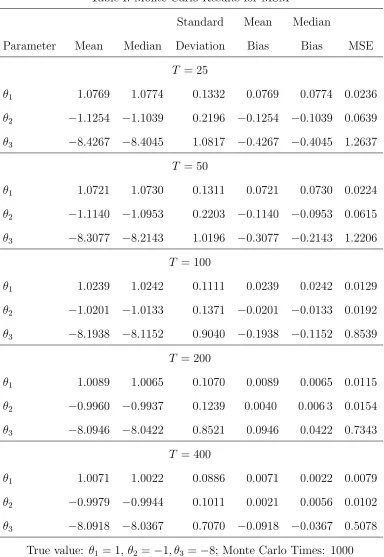
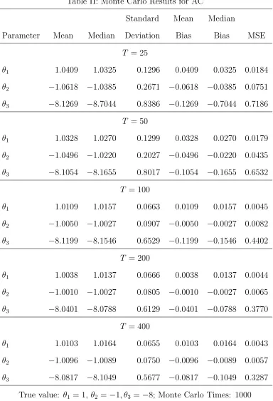
In Table I we report the mean, median, standard deviation, mean bias, median bias and mean square error (MSE) for the MSM estimator defined in (13) for five sample sizes,
T = 25,50,100,200 and 400 and Table II for the AC estimator defined in (14), which show that both estimators can perform well in moderately-sized samples, the payoff parameters are estimated near their true values, and as the sample size increase, the estimates become more precisely. The comparison between the MSM estimator and AC estimator shows the superiority of AC estimator, especially in small samples. One may find that parameters are estimated much less precision when sample size is 400, this may due to the large scale non-linear algorithm we’ve chosen. Actually, since the objective function of our estimate is not globally convex, we choose the global optimization algorithm ”LGO”6
in GAMS, a more meticulous modification on the algorithm details should increase the performance of our estimation in large samples.
6
Table I: Monte Carlo Results for MSM
Standard Mean Median
Parameter Mean Median Deviation Bias Bias MSE
T = 25
θ1 1.0769 1.0774 0.1332 0.0769 0.0774 0.0236
θ2 −1.1254 −1.1039 0.2196 −0.1254 −0.1039 0.0639
θ3 −8.4267 −8.4045 1.0817 −0.4267 −0.4045 1.2637
T = 50
θ1 1.0721 1.0730 0.1311 0.0721 0.0730 0.0224
θ2 −1.1140 −1.0953 0.2203 −0.1140 −0.0953 0.0615
θ3 −8.3077 −8.2143 1.0196 −0.3077 −0.2143 1.2206
T = 100
θ1 1.0239 1.0242 0.1111 0.0239 0.0242 0.0129
θ2 −1.0201 −1.0133 0.1371 −0.0201 −0.0133 0.0192
θ3 −8.1938 −8.1152 0.9040 −0.1938 −0.1152 0.8539
T = 200
θ1 1.0089 1.0065 0.1070 0.0089 0.0065 0.0115
θ2 −0.9960 −0.9937 0.1239 0.0040 0.006 3 0.0154
θ3 −8.0946 −8.0422 0.8521 0.0946 0.0422 0.7343
T = 400
θ1 1.0071 1.0022 0.0886 0.0071 0.0022 0.0079
θ2 −0.9979 −0.9944 0.1011 0.0021 0.0056 0.0102
θ3 −8.0918 −8.0367 0.7070 −0.0918 −0.0367 0.5078
Table II: Monte Carlo Results for AC
Standard Mean Median
Parameter Mean Median Deviation Bias Bias MSE
T = 25
θ1 1.0409 1.0325 0.1296 0.0409 0.0325 0.0184
θ2 −1.0618 −1.0385 0.2671 −0.0618 −0.0385 0.0751
θ3 −8.1269 −8.7044 0.8386 −0.1269 −0.7044 0.7186
T = 50
θ1 1.0328 1.0270 0.1299 0.0328 0.0270 0.0179
θ2 −1.0496 −1.0220 0.2027 −0.0496 −0.0220 0.0435
θ3 −8.1054 −8.1655 0.8017 −0.1054 −0.1655 0.6532
T = 100
θ1 1.0109 1.0157 0.0663 0.0109 0.0157 0.0045
θ2 −1.0050 −1.0027 0.0907 −0.0050 −0.0027 0.0082
θ3 −8.1199 −8.1546 0.6529 −0.1199 −0.1546 0.4402
T = 200
θ1 1.0038 1.0137 0.0666 0.0038 0.0137 0.0044
θ2 −1.0010 −1.0027 0.0805 −0.0010 −0.0027 0.0065
θ3 −8.0401 −8.0788 0.6129 −0.0401 −0.0788 0.3770
T = 400
θ1 1.0103 1.0164 0.0655 0.0103 0.0164 0.0043
θ2 −1.0096 −1.0089 0.0750 −0.0096 −0.0089 0.0057
θ3 −8.0817 −8.1049 0.5677 −0.0817 −0.1049 0.3287
5
CONCLUSION
References
Aguirregabiria, V. & P. Mira (2007). ”Sequential Estimation of Dynamic Discrete Games.”
Econometrica 75 : 1-53.
Ackerberg, D. A. (2009). ”A New Use of Importance Sampling to Reduce Computational Burden in Simulation Estimation.” Quantitative Marketing and Economics 7 (4): 343– 376.
Bajari, P. & H. Hong, et al. (2010). ”Estimating Static Models of Strategic Interactions.” forthcoming Journal of Business and Economic Statistics.
Bajari, P. Han Hong & Stephen Ryan (2010). ”Identification and Estimation of a Discrete Game of Complete Information.” forthcoming Econometrica.
Berry, Steven T. (1992). ”Estimation of a Model of Entry in the Airline Industry.” Econo-metrica 60 (4): 889-917.
Berry, Steven T. & Tamer, E. (2007). ”Identification in Models of Oligopoly Entry.” in Advanced in Economics and Econometrics: Theory and Application, vol. II, chap. 2, pp.46-85. Cambridge University Press, Ninth World Congress.
Bresnahan, T. F. & P. C. Reiss (1990). ”Entry in Monopoly Markets.”Review of Economic Studies 57 : 531-553.
Bresnahan, T. F. & P. C. Reiss (1991). ”Empirical models of Discrete Games.” Journal of Econometrics 48 : 57-81.
Ciliberto & Tamer, E. (2009). ”Market Structure and Multiple Equilibria.”Econometrica, 77 (6): 1791-1828.
Dominguez, M. A. & I. N. Lobato (2004). ”Consistent Estimation of Models Defined by Conditional Moment Restrictions.”Econometrica 72 (5): 1601-1615.
Christian Gouri´eoux & Alain Monfort (2002).Simulation-based econometric methods. Ox-ford university press.
Haile, P., & A. Hortacsu, et al. (2003). ”On the Empirical Content of Quantal Response Equilibrium.” Working Paper.
Hansen, L. P. (1982). ”Large Sample Properties of Generalized Method of Moments Es-timators.” Econometrica 50 (4): 1029-54.
Aradillas-Lopez (2007). ”Pairwise Difference Estimation of Incomplete Information Games.” Working Paper.
Aradillas-Lopez (2008). ”Semiparametric Estimation of a Simultaneous Game with In-complete Information.” Working Paper.
Maruyama, S. (2009). ”Estimating Sequential-move Games by a Recursive Conditioning Simulator.” Working Paper.
Mazzeo, Michael J. (2002). ”Product Choice and Oligopoly Market Structure.” Rand Journal of Economics 33 (2): 221-242.
Martin J. Osborne & Ariel Rubinstein. (1994).A Coure in Game Theory. The MIT Press.
McFadden, D. (1989). ”A Method of Simulated Moments for Estimation of Discrete Re-sponse Models without Numerical Integration.” Econometrica 57 (5): 995-1026.
Klaus Ritzberger (2002).Foundations of Non-Cooperative Game Theory. Oxford Univer-sity Press.
Pakes, A. & D. Pollard (1989). ”Simulation and the Asymptotics of Optimization Esti-mators.” Econometrica 57 (5): 1027-57.
Schmidt-Dengler, P. (2006). ”The Timing of New Technology Adoption: The Case of MRI.” Working Paper.
Seim,. K. (2005). ”An Empirical Model of Firm Entry with Endogenous Product-Type Choices.” Rand Journal of Economics 37 (3): 619-640.
Tamer, E. (2003). ”Coordination Games, Multiple Equilibria and the Timing of Radio Commercials.” Working Paper.