A novel kernel PLS method for object tracking

Journal of Chemical and Pharmaceutical Research, 2014, 6(7):659-669

Research Article

_{CODEN(USA) : JCPRC5}

ISSN : 0975-7384

A novel kernel-PLS method for object tracking

Yi Ouyang*, Yun Ling and Biyan Wu

School of Computer and Information Engineering, Zhejiang Gongshang University, Hangzhou, China

___________________________________________________________________________________________

ABSTRACT

In this paper, we propose a On-line kernel-PLS approach to improving both the robustness and accuracy of object tracking which is appropriate for real-time video surveillance. Typical tracking with color histogram matching provides robustness but has insufficient accuracy, because it does not involve spatial information. On the other hand, tracking with pixel-wise matching achieves accurate performance but is not robust against deformation of a target object. To tackle these problems, this paper presents a tracking method that combine histogram-wise matching and pixel-wise template matching via leans a robust object representation by Kernel-PLS analysis and adapts to appearance change of the target. In this paper, we propose a novel On-line Kernel-PLS analysis, for generating a low-dimensional discriminative feature subspace. As object appearance is temporally correlated and likely to repeat over time, we learn and adapt multiple appearance models with On-line Kernel-PLS analysis for robust tracking. Key words: Image processing; PLS; Object Tracking; Classification; Feature spaces

_____________________________________________________________________________________________

INTRODUCTION

Target tracking has been an important topic in computer vision for several years. Recent years have been significant progress in tracking. To distinguish targets with backgrounds and with each other, most visual tracking methods focus on tracking target appearance separately; they usually try to find proper appearance models that distinguish object with all other targets or backgrounds, and adopt meanshift or particle filtering like approach to online adjust target appearance models, and use updated models to continuously track targets.

The most tracking methods reported to handle this difficulty, thus far, is to adaptively update the target appearance model at each frame: learn a new appearance model with time invariant characteristics extracted from historic observed target samples, and adopt the model to the current frame. Such as, IVT [1] algorithm uses a subspace model by adding adaptively modify the appearance of the model. Tracking-Learning-Detection (TLD) [2] method to track task is decomposed into three sub-processes: tracking, learning and learning, each sub- task as a separate task , each sub-task can be performed s tracking will fail . (2 ) the target disappeared, detection operator continues . (3 ) less real-time tracking and other issues . In order to solve the above problems , Kalal [3] analyze a variety of information in video images and proposed a new learning framework called P-N Learning for training a binary classifier from labeled and unlabeled examples. The learning process is guided by positive experts and negative experts constraints which restrict the labeling of the unlabeled set. P-N learning evaluates the classifier on the unlabeled data, identifies examples that have been classified in contradiction with structural constraints and augments the training set with the corrected samples in an iterative process. Learning processes for any errors exist , the expert operator P-N due to mutual compensation of the error probability is limited within a certain range in order to achieve stability. Based on P-N learning method, Saigo [4] proposed PLS method to obtain a better target tracking. The Fragment-based tracker [11] aims to solve partial occlusion with a representation based on histograms of local patches. The tracking task is carried out by combing votes of matching local patches using a template. There are some sparse matrixes combined with particle filter for target tracking applications L1 [5].

(KPCA)[16] and Kernel-Partial Least Squares analysis (KPLS) [17,18] have previously been applied in a multitude of contexts for exploratory analysis and classification, including biological applications [19].

Target tracking problem is challenging as tracking processing needs to deal with appearance variations caused by many factors such as illumination, pose deformation, occlusion, background clutter, and camera motion. This paper focuses on the issue of nonlinear K PLS analysis for target tracking. To tackle these challenges, we present a tracking method that learns a robust object representation by Kernel partial least squares analysis and adapts to appearance change of the target. Firstly, we extend these earlier works[4] by embedding nonlinear kernel analysis for PLS tracking. To improve the existing work, we perform the color histogram probability density function for the object color constraint is modeled as a smooth function that indicates how well the candidate set images and target is met. To improve stability for standard belief propagation, the color constraint function node is connected to four gradient variable nodes.

Although detection results can be improved by utilizing overlapping blocks for low-level feature extraction within the detection window, the dimensionality of the feature vector becomes extremely high. As a result, the speed of the human detector decreases significantly due to the time needed to extract features and project them. To overcome this problem, we employ a On-line learning approach. In a fast first stage, based on a small number of features, the majority of detection windows (those with low probability of containing humans) are discarded. The remaining windows are evaluated during a second stage where the complete set of features allows challenging samples to be correctly classified.

ON-LINE KERNEL-PLS ANALYSIS(KPLS)

The PLS method employs the descriptor matrix

X

∈

R

N K× , where N denotes the number of samples and K the number of variables in X, to predict the response matrix

Y

∈

R

N M× , where M denotes the number of variables in Y. The unique property of the PLS method compared to other linear regression methods is its ability to separate the modeling of covariation from structured noise, defined as systematic Y-orthogonal variation, while simultaneously maxim the covariance between X and Y.

The K-PLS algorithm follows the principles of the linear PLS algorithm while it is written in dual form. This implies

that all expressions have been rewritten so that the input matrix X is expressed as the outer product

XX

T in all instances. The outer product

XX

T is subsequently replaced by the kernel matrix K in the K-PLS algorithm. K is deflated for the Y-orthogonal components. In simple terms, in the algorithm for model estimation, K consists of two instances of the transformed data matrix. One of these instances represents the predictive weights W and should thus be retained throughout the calculations, whereas the other should be deflated accordingly by the Y-orthogonal

variation. Subsequently,

XX

T

is substituted for the kernel Gram matrix K with entries

K

i j,

=

k x x

( ,

i j

)

_{, where}

x

i _and

x

j _{corresponds to the i-th}

and j-th row vector in the descriptor matrix X, respectively, and

k x x

( ,

i j

)

represents the kernel function. Hence, one can avoid explicitly mapping X to higher-dimensional spaces as well as computing dot products in the feature space, which is computationally beneficial. The transformation to higher dimensional spaces is performed implicitly by the kernel

function

k x x

( ,

i j

)

; where common kernel functions use Gaussian functions as follow:

2 2

( , )

( ||

|| /2

)

k x y

=

exp

−

x

−

y

σ

_(0.1)

stage is given by the vector

u

j, which is in the primal space while we must work in dual space,and express a multiple

of

u

j as

T j j j j

a u

=

X

β

(0.2)

which is clearly consistent with the derivation of

u

j in the primal PLS algorithm. For the dual PLS algorithm we must implement the deflation of Y. This redundant step for the primal will be needed to get the required dual

representations. We use

Y

j _{to denote the j-th deflation.}

T T T

j j j j j j j

Y Y X X

Y Y K

β

=

β

=

β

_(0.3)

with the normalization

||

||

β

β

β

=

,then compute a rescaled

t

j _and

c

j_. T

j j j j j j j j j

T T

j j j j j j

j T T T

j j j j j j j j

t

a X u

X X

K

Y t

Y X u

c

c

t t

a u X X u

a

β

β

′

=

=

=

=

=

=

(0.4)

where

c

j′ denotes the same weight vectors c in PLS algorithm.

t

j can be consider as a rescaled dual representation of the output vector

c

j′.

Let

u v

j

,

j

,

σ

j be the first singular vector of

T j

X Y

,the deflation of

X

j as

1

(

)

T j j

j T j

j j

t t

X

I

X

t t

+

= −

(0.5)

with an equivalent deflation of the kernel matrix

1 1 1

(

)

(

)

T T

j j j j T

j j j T j T

j j j j

t t

t t

K

X

X

I

K I

t t

t t

+

=

+ +

= −

−

(0.6)

In this paper, we formulate object tracking as a classification problem with On-line Kernel PLS analysis to learn a low-dimensional and discriminative feature subspace. S.Wold et al. [12,13]were the first to extend the linear PLS model to its nonlinear form. They have done this by replacing the linear inner relation between the score vectors t and u by a nonlinear model.

( )

( , )

u

=

k t

+ =

e

k X w

+

e

_(0.7)

where k represents a continuous nonlinear function,

e

denotes a vector of residuals. The relation between each pair of latent variables is modeled separately. We use radial basis function to model k. It can be observed that the vector of weights of

w

, computed in the first step of the NIPALS algorithm, represents the sample covariance between the

output space score vector

u

and the input space data matrix

X

. However, the use of a nonlinear model to relate the score vectors in the inner relation affects the computation of

w

. Although w represents the association among variables of X and u also in nonlinear PLS, this association will be closely related to covariance values only if the nonlinear mapping between latent variables is monotonic and slightly nonlinear.

used to update w. So, consider the nonlinear inner relation, where

k t

( )

=

k X w

( , )

is continuous and differentiable with respect to w. The second-order Taylor expansion of has the form

0

ˆ

k

u

u

w

w

∂

= +

∂

(0.8)

where

u

0

=

k t

( )

_{is the value of g at the known value of t. Similarly,}

k

w

∂

∂

stands for the partial derivatives of g numerically evaluated at the same known value of t. The second term of 12 can be written element-wise as

1 N i i

k

k

w

w

₌

w

∂

₌

∂

∂

∑

∂

_(0.9)

At this point several different methods to compute the correction

w

were proposed. To simplify further notation

consider the matrix form of the linear approximation

u

ˆ

ˆ

u

=

Zv

_(0.10)

where

0

[

k

]

Z

u

w

∂

=

∂

and

[1

]

T

v

=

w

_{. The following variants to compute}

_w

_{were suggested:}

1

( , )

( ) ( )

( )

( )

( ),

( )

D T i i

k x y

x

y

x

y

x

y

α φ φ

=

=

= Φ

Φ

=< Φ

Φ

>

∑

(0.11)

where

{ }

φ

i _{is a sequence of linearly independent functions,}

{ }

α

i _{are positive numbers and}

D

≤

N

_{is the}

dimension of the space H. Following this relation the feature map

Φ

can be written as

: X

F

Φ

→

(0.12)

1 1 2 2

( )

(

( ),

( ),...,

_{N N}

( ))

x

→ Φ

x

=

a

φ

x

a

φ

x

a

φ

x

(0.13)

Thus, if we are only interested in the computation of dot products in F, it does not matter how F was constructed and simply all dot products can be replaced by a unique kernel function associated with F . This is important to note because different feature spaces associated with the same kernel function can be constructed. In literature, this replacement of a dot product with the kernel function value is known as the kernel trick method.

A modified version of the NIPALS algorithm where steps 1 and 3 are merged and the score vectors t and u are scaled to unit norm instead of scaling the weight vectors w and c. The obtained kernel form of the NIPALS algorithm is as follows

Step1:

t

= ΦΦ =

T

u

Ku

Step2:

|| ||

t

→

1

Step3:

c

=

Y t

T Step4:

u

=

Yc

Step5:

|| ||

u

→

1

applications where an analogous kernel mapping

Φ

of the Y-space data is considered; that is, the Gram matrix

T y

K

= ΦΦ

of the cross dot products between all mapped output data is constructed. Then, the kernel NIPALS algorithm consists of the following four steps. Step 3 and 4 can be further merged which may become useful in applications where an analogous kernel mapping

Φ

of the Y-space data is considered; that is the Gram matrix

T y

K

= ΦΦ

of the cross dot products between all mapped output data is constructed. Then, the kernel NIPALS algorithm consists of the following four steps

Step1:

t

=

Ku

Step2:

|| ||

t

→

1

Step3:

u

=

K t

y Step4:

|| ||

u

→

1

The On-line KPLS algorithm learns a threshold in linear function in a kernel-defined feature space.

( )

, ( )

h x

=

sgn

<

w

φ

x

>

_(0.14)

If the weight vector after t updates is denoted by

w

t _{then the update rule for the (t+1) update when an sample}

( ,

x y

_{i i}

)

is misclassified is given by

1

( )

t t i

w

₊

=

w

+

y

φ

x

(0.15)

Hence, the corresponding dual update rule is simple

1

i i

a

= +

a

(0.16)

if we assume that the weight vector is expressed as

1

( )

N

t i i i i

w

a y

φ

x

=

=

∑

(0.17)

Once the weight matrix

W

=

[

w

1

,...,

w

k

]

_{is computed, the initial appearance model can be denoted by} 1

{

p

, ,

ˆ

}

A

=

x x W

, where

x

p _{is the mean of the positive samples. A test sample,}

x

∈

R

m_{, can be projected onto the}

learned latent feature space specified by

A

1 _{to get a latent feature vector}

(

ˆ

)

T

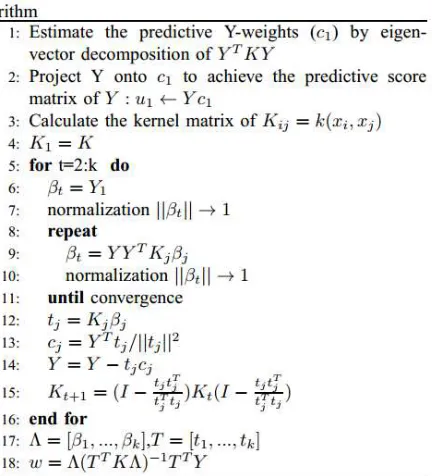
[image:6.595.199.415.87.325.2]

Figure 1.Pseudo-code for the On-line KPLS algorithm

TARGET APPEARANCE MODEL

Since the appearance change of an object during a long period of time may be quite nonlinear and complex, one linear appearance model is not likely to suffice. However, appearance of a target object may be temporally correlated and may repeat over time. We therefore learn multiple appearance models for more effective object representation.

Video sequence of a target over a long period can be divided into multiple sets. Within the i-th set, the object appearance dosed not change much and we use KPLS analysis to learn a discriminative appearance model

{

p

, ,

}

i i i i

A

=

x

x W

. Therefore, the appearance of a target object can be represented by multiple appearance models

1

{ ,...,

_k

}

A

=

A

A

, where k is the number of appearance models. The proposed representation scheme is more effective than existing methods base on single linear appearance model.

In this paper, the distance between a test sample

x

∈

R

m and the learned appearance model set A is defined as

2 2 1

| |

(

)

(

) ||

k

T T p

i i

i

Dist

W

x

x

W

x

x

=

=

∑

− −

−

(0.18)

where

x

p is the mean of the positive samples used in training

A

i_,

x

i _{is the mean of all the samples in training}

A

i_,

and

|| . ||

2 _{is Euclidean norm.}

The target and background appearances may change due to factors such as illumination, pose, occlusion, camera motion, and so on. To deal with this problem, we propose an adaptive object representation method. Let the current set

of appearance models be

A

=

{

A i

i

|

=

1,..., ,

k k

≤

K

}

_.

When the tracking result at time t is obtained, we use the corresponding target observation

x

t _{to update}

A

_{. Since we}

have computed the distances from the target observation

x

t _{to all the appearance models in}

A

_{for determining the}

tracking result, we select the appearance model

A

s _{with the smallest distance}

d

s _{and the appearance model}

A

l

The update process includes three components: the mean of the positive sample

p i

x

,the mean of all the training

samples

x

, and the weight matrix

W

.

x

p can be updated by using a random update probability.

Both

ˆx

and

W

can be updated by KPLS method with the positive and negative samples. If

||

A

s

−

A

l

||

_{is larger}

than the predefined threshold and

k

<

K

, a new appearance model

A

k+1 _{is added to A. If}

||

A

s

−

A

l

||

_{is larger}

than the predefined threshold and

k

=

K

, a new appearance model is initialized to replace

A

l _{in A. The proposed}

adaptive appearance model is summarized as follow:

Figure 2.Adaptive Appearance Model Based on KPLS analysis

ON-LINE KPLS TRACKING METHOD VIA MAP

Given the observation set of the target

x

1:t

=

[ ,... ]

x

1

x

t _{up to time t, the tracking result}

s

t _{can be determined by the}

Maximum A Posteriori (MAP) estimation,

1:

( |

)

t t t

s

=

argmax p s x

(0.19)

where

p s x

( |

t 1:t

)

_{is inferred by the Bayes}

theorem recursively with follow equation.

1: 1:

( |

_{t t}

)

(

_t

| ) ( |

_{t t t}

)

p s x

∝

p x s p s x

(0.20)

1: 1 1 1 1: 1 1

( |

_{t t}

)

(

|

_t

) (

_t

|

_t

)

_t

p s

x

₋

=

∫

p s t s

−

₋

p s

₋

x

₋

ds

₋

This inference is governed by the dynamic model

p s s

( |

t 1: 1t−

)

_{which describes the temporal correlation of the}

tracking results in consecutive frames, and the likelihood function (i.e., observation model)

p x s

(

t

| )

t _which

denotes the likelihood of

s

t _observing

x

t _.

The main issue for any adaptive appearance model is that it is likely to use noisy or mis-aligned observations for update, thereby causing tracking drift gradually. For online tracking, the only ground truth at our disposal is the labeled target object in the first frame.

Let X as random variable of a video sequence, defining the state vector

X

t

=

{

L

( , )x y

, }

s

t ,where

L

( , )x y is the target center location,

s

t _{is the scale factor,}

p y x

(

t

| )

_{denotes the probability of cliques belongs to target. Motion model}

1

(

_t

|

_t

)

p x x

₋

generate a predict x, which denotes the correlation of target's temporal structure in the video. We assume that the motion model obeys Gaussian distribution:

1 1

(

_t

|

_t

)

( ( ,

_{t t}

), )

p x x

₋

=

N m x x

₋

Λ

(0.22)

where

Λ

is the diagonal covariance matrix,

m x x

( ,

t t−1 _{denotes the means of two random variable. We use Bayes}

filtering method to track target .

Prediction stage:

1 1 1

( )

(

_t

|

_t

)

(

_t

)

_t

Bel x

=

∫

p x x

₋

Bel x

₋

dx

₋

Update stage:

( )

_{t t}

(

_t

|

_t

)

( )

_t

Bel x

∝

a p y x Bel x

Observation Markov assumptions: Observation depends only on the state of the current observations, i.e.

1: 1: 1

(

_t

|

_t

)

(

_t

|

_t

) (

_t

|

_t

)

p y

x

=

p y x p z

₋

x

, the filtering process is mainly determined by the dynamic model

1

(

_t

|

_t

)

p x x

₋

, which describes the state temporal correlation of the target between frames .

EXPERIMENTAL ANALYSIS

To evaluate On-line KPLS, we compile a set of 15 challenging tracking sequences (e.g. car4, woman) that are publicly available online. Due to space constraints, we will only show results on 4 of these sequences. These videos are recorded in indoor and outdoor environments and include challenging appearance variations due to changes in pose, illumination, scale, and the presence of occlusion. The center distance error results of proposed tracking method are compared with that of current state-of-the-art methods IVT [1], TLD [2], LOT [7] and ROT [8]. Experimental video sequences singer1 and basketball from VTD[9], lemming and liquor from PROST[10], woman from FragTrack[11] and girl_mov from SPT [6]. Implemented in MATLAB on an Intel Core 2.26 GHz computer with 4GB RAM and no code optimization.

Table 1. The mean of Center D denote average errors of center position

Seq\Method IVT TLD SPT LOT ROT OUR

Basketball 94 7 5 6 6 7

Girl_mov 216 128 26 36 105 31

Bolt 83 - 7 12 150 25

Liquor 54 30 8 9 34 12

[image:9.595.77.539.67.436.2] [image:9.595.154.432.464.696.2]

woman girl_mov basketball liquor

Figure 3. Tracking results comparison during tracking process

Figure 4. CDE results comparison during tracking process

tracking method considers local and environmental features surrounding, and adaptively adjusting the target appearance model, which can more accurately distinguish target and improve tracking accuracy.

In Figure3 basketball sequence, because the target of the block is not serious, the proposed method and SPT almost unanimously, in girl_mov, when traced to 115. In liquor object appears in a similar situation, the proposed method with SPT similar. The presence of the target under occlusion, the proposed method is superior to other methods.

In Table-1and Figure 4, the paper uses Center Distance Error (CDE)to analysis the tracking performance, where '-' indicates partial frame detection failure tracking process.CDE represents the center position coordinates errors between the tracking results and the reference standard (ground truth) , where$||.||$ is the Euler distance, '-' indicates some frames tracking failure in the tracking process.

The target objects are partially occluded in the woman sequences, which has a partially occlusion phenomenon. Using On-line KPLS method can eliminate the target because of changes in background appearance model for the impact, and the adaptive appearance learning approach through dynamic update appearance models, target tracking accuracy of better than TLD, IVT, LOT and ROT methods to detect and deal with serious obscured targets.

The results (Figure 4) show that it is normal condition in the center and the ground truth detection frame error is basically the same, when there is heavy occlusion, our method is significantly better than other tracking algorithms.

CONCLUSION

This paper presents a novel On-line Kernel PLS analysis method for object tracking, and utilizes the positive samples and negative samples for adaptively updated information on the target - background appearance model. To solving the these problems, such as occlusion, illumination changing, and the shape changing during the process of the target tracking. We employ the image KPLS weight scores as confidence response map to determine the target location information. Although traditional tracking method tracking detection results can be improved by utilizing overlapping blocks for low-level feature extraction within the detection window, the dimensionality of the feature vector becomes extremely high. As a result, the speed of the human detector decreases significantly due to the time needed to extract features and project them.

To overcome this problem, we employ a On-line learning approach. In a fast first stage, based on a small number of features, the majority of detection windows (those with low probability of containing humans) are discarded. The remaining windows are evaluated during a second stage where the complete set of features allows challenging samples to be correctly classified.

Acknowledgment

The authors would like to thanks the anonymous reviewers for their constructive and useful comments, which helped in improving the presentation of our work.

REFERENCES

[1]Ross D A ,Lim J , Lin R S, et al. International Journal of Computer Vision, 2008, 77(1-3): 125-141.

[2]Kalal Z, Mikolajczyk K and Matas J. IEEE Transactions on. 2012, 34(7): 1409-1422.

[3]Kalal Z ,Matas J and Mikolajczyk K. Pn learning: Bootstrapping binary classifiers by structural constraints, Computer Vision and Pattern Recognition (CVPR), 2010 IEEE Conference on, 2010: 49-56.

[4]Saigo H, Kr mer N and Tsuda K. Partial least squares regression for graph mining. Proceedings of the 14th ACM SIGKDD international conference on Knowledge discovery and data mining, 2008: 578-586.

[5]Wang Yu-Xiang, Xu Han and Ma Ting-Huai. Journal of Electronics & Information Technology,2012,V34(1): 223-226.

[6]Wang S ,Lu H and Yang F, et al. Superpixel tracking[C].Computer Vision (ICCV), 2011 IEEE International Conference on, 2011: 1323-1330.

[7]Oron S ,Bar-Hillel A and Levi D, et al. Locally orderless tracking. Computer Vision and Pattern Recognition (CVPR), 2012 IEEE Conference on, 2012: 1940-1947.

[8]Ning J, Zhang L, Zhang D and Wu C. Robust object tracking using joint color-texture histogram. International Journal of Pattern Recognition and Artificial Intelligence. 2009, 23(07): 1245-1263.

[9]Kwon J and Lee K M. Visual tracking decomposition. Computer Vision and Pattern Recognition (CVPR), 2010 IEEE Conference on, 2010: 1269-1276.

[11]Adam A ,Rivlin E and Shimshoni I. Robust Fragments-based Tracking using the Integral Histogram.Computer Vision and Pattern Recognition 2006 IEEE Computer Society Conference on, 2006:798-805.

[12]Trygg J, Wold S. Journal Chemometrics,2002, 16:119-128.

[13]Trygg J, Wold S. Journal Chemometrics,2003, 17:53-64

[14]Shawe-Taylor J, Cristianini N: Kernel methods for pattern analysis, Cambridge University Press; 2004:462.

[15] Schölkopf B, Smola A: Learning with Kernels: Support Vector Machines, Regularization, Optimization, and Beyond.Cambridge , MIT Press; 2001.

[16]Rosipal R, Girolami M,Trejo LJ, Cichocki A: Neural Comput Appl 2001, 10(3):231-243.

[17]Lindgren F, Geladi P, Wold S: Journal Chemometrics,1993, 7(1):45-59.

[18]Rosipal R, Trejo LJ: J Mach Learn Res,2002,2(2):97-123.