Number 6180
Konkoly Observatory Budapest
18 August 2016 HU ISSN 0374 – 0676
RW ARIETIS, AN ECLIPSING RR LYRAE STAR?
ODELL, ANDREW P.1; SREEDHAR, Y. HARSHA2 1
Dept of Physics and Astronomy, Northern Arizona University, Flagstaff, AZ 86011, USA, e-mail: [email protected]
2
Indian Institute of Astrophysics, Koramangala, Bangalore 560034, India, e-mail: [email protected]
1
Introduction
RW Arietis is a typical RRc star, thus a core-helium burning, post-RGB star pulsating in the radial first overtone (period ≈ 0.3543 days, amplitude in V ≈ 0.540 mag); normally
these stars have a stable period and light curve behavior. Variability of the star was discovered by Detre (1937), who found an alias (0.26141 days) of the true period, which was corrected by Notni (1962) to 0.3543184 days.
Wi´sniewski (1971) brought attention to RW Ari when he announced what appeared to be eclipses on three of his 19 nights of photoelectric observations in 1966-71. He suggested an orbital period of 3.1754 days, with the companion star being perhaps a blue giant or young B-type star, based on eclipse depth and color change. He acknowledged that this is difficult to understand, since the RR Lyr component would have gone through the red giant phase, and presumably destroyed a close companion. However, Wi´snewski should have noticed that on another night when a primary eclipse was expected, it was not seen, and a bright blue companion would have diluted the pulsation amplitude, also not seen.
Abt & Wi´sniewski (1972) searched for evidence of orbital motion by obtaining spectra of RW Ari at presumably the same pulsation phase, but separated by half the purported orbital period, and found a radial velocity difference of 35 km s−1. Unbeknown to these
authors, the pulsation period had changed and their phasing was not correct (see sections 3 and 5). Also in response to Wi´snewski’s claim, Edwards (1978) and Goranskij & Shugarov (1979) (GS79 in tables) separately undertook photometric observations to confirm or deny the 3.17 days period, both ruling out that possibility.
If confirmed, RW Ari would be the first true RR Lyr star in an eclipsing binary. Others have been suggested, including TU UMa, VX Her, RZ Cet, and OGLE-BLG-02792; the first has a possible period of 23 years, the second and third have not been confirmed, and the final one has a mass much too small to be a classical RR Lyr star (see Liska 2016). The observation of a mass and radius could resolve the discrepancy between RR Lyr masses derived from stellar evolutionary and pulsation models.
1
We realized that a wealth of photometric measurements exists in surveys (such as Super-WASP), and that if eclipses occur with any short period, evidence should be easy to obtain from them. In addition, Lowell Observatory agreed to use its robotic NASAcam to visit the star once per hour to also attempt to discover eclipses. No further eclipses were seen in any of the data sets (see section 2). This allows us to put a lower limit on the orbital period of at least 25 days, and almost certainly eliminate one longer than this, as well.
Since we have many new timings of maximum and minimum light, as well as excellent light and radial velocity curves, we decided to collect all this information and make it available to the community, which is the purpose of this paper (see sections 3, 4, and 5).
2
Attempt to Find Eclipses
[image:2.595.190.409.416.562.2]Wi´sniewski (1971) claimed that RW Ari exhibited an eclipse ingress on April 16, 1966 (JD 2439384) that lasted for two hours. He advocated an orbital period of 3.1754 days based on two additional nights that might have shown a primary and a secondary eclipse, but this was ruled out by two subsequent studies: Edwards (1978) and GS79. However, these studies left open the the possibility that some other period might be appropriate, but with no idea when to observe again. We realized that several all-sky survey archives could be searched for evidence of eclipses, and with very little effort. Table 1 lists all the sources of photometric data we could find.
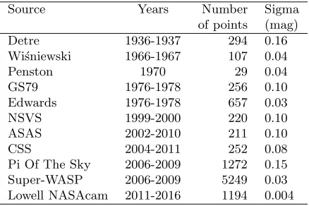
Table 1. Photometric Datasets
Source Years Number Sigma of points (mag) Detre 1936-1937 294 0.16 Wi´sniewski 1966-1967 107 0.04 Penston 1970 29 0.04 GS79 1976-1978 256 0.10 Edwards 1976-1978 657 0.03 NSVS 1999-2000 220 0.10 ASAS 2002-2010 211 0.10 CSS 2004-2011 252 0.08 Pi Of The Sky 2006-2009 1272 0.15 Super-WASP 2006-2009 5249 0.03 Lowell NASAcam 2011-2016 1194 0.004
NSVS = Northern Sky Variability Survey (Wozniak et al. 2004) ASAS = All Sky Automated Survey (Pojmanski 2002)
CSS = Catalina Sky Survey (Drake et al. 2014) Pi Of The Sky (Mankiewicz et al., 2014)
The survey with the highest quality and quantity of photometry is the Super-WASP (Wide Angle Search for Planets; see Pollacco et al. 2006). Richard West (personal comm.) graciously and quickly supplied over 3000 useful measures from the 2006-7 season, and another 2200 from 2008-9. Unfortunately, after eliminating the measures with greater than 5% error, no obvious deviations from the RR Lyr light curve emerged.
Our entire set of photometric observations are given in Table 8, as HJD and magni-tude: (for filters B, V, R, and I). (The table is available through the IBVS website as
6180-t8.txt.) Since the Super-WASP data has not been released for stars within 20◦ of
the equator, we also make available that photometry in Table 9, as HJD and unfiltered magnitude. (This table is also available through the IBVS website as 6180-t9.txt.)
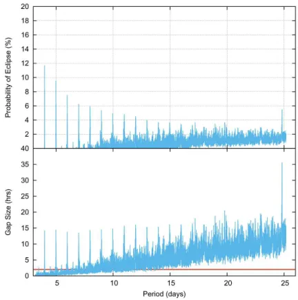
This lack of eclipses meant we could not find an orbital period or predict another eclipse. So we decided to see what periods we could eliminate with this data set, by writing a FORTRAN program which would consider periods starting at Wi´sniewski’s 3.17 days, and work upward, folding the SuperWASP and NASAcam times of no eclipse, and looking for the largest gap in time. The trial period was incremented by 0.14 minute up to 5.17 days, and then 1.4 minutes up to 25 days.
[image:3.595.165.381.414.631.2]The lower panel of Fig. 1 shows the largest gap (in hours) in a possible light curve as a function of period. If the gap is less than three hours, then that assumed period can be ruled out. With longer gaps, the probability of an eclipse being able to hide in them can be estimated as the length of the gap, minus three hours, divided by the period, which is displayed in Fig. 1 top panel. Large gaps appear at exact integer numbers of days, as the eclipse could take place always during daylight hours. So, for example, if the period were exactly 5.0 days, the largest gap would be about 10 hours, during daylight, and the eclipse missed. If the period were just 1.5 minutes longer or shorter than 5.0 days, the eclipse would migrate into the night, and have been observed sometime during our coverage. However, the probability the orbital period would be that close to 5.0 days is at the 0.02% level.
Figure 1. Bottom panel - the size of the largest gap in hours, as a function of assumed (folding) period in days. Top panel - the probability of missing an eclipse (percentage which the largest gap (minus 3
hours) is, of the assumed period).
A much longer orbital period cannot be ruled out; indeed it becomes more likely, due to larger uncovered gaps. However, it also becomes much less likely that the orbit would be oriented edge-on to the level necessary. Discouraged by this eventuality, we decided to study the RR Lyr pulsations instead, to which the rest of this paper is devoted.
3
Pulsation Period Changes and Ephemeris
3.1 Ephemeris for the timings from Lowell Observatory
In anticipation of finding eclipses for RW Ari which would affect the RR Lyr light curve, we decided to obtain a full, high quality light curve in BVRI on 21 October, 2011 with Lowell Observatory’s NASAcam (see section 3). We continued to record full light curves on additional nights, to monitor any period or light curve changes. While many light curves have been made over the years, there has been a problem fitting all of them with one period (see Todoran 1988). Ultimately we derived timings of maximum and/or minimum light on 13 additional nights between 2011 and 2016, as well as a few timings from the B
filter alone (details given in section 3).
The light curve of RW Ari seems to remain quite constant over the years, but it has a very broad maximum (see section 3). Thus we determined that minimum light occurs at phase 0.55, and used timings of that as well, adjusting the cycle count by that fraction. The method of finding the time of maximum or minimum is a method developed for eclipsing binary stars by Kwee & van Woerden (1956). Essentially the light curve is folded about a time, so the rising branch falls over the descending branch, and the folding time adjusted to obtain the best correlation (here done by eye). In a few instances, maximum or minimum was not well covered, and the timing was determined by overlaying the phased light curve with the night of 26 September, 2013 as a template, and adjusting the assumed phase zero time until the two curves coincided optimally.
Our results are shown in Table 2, where the estimated cycle number E, HJD, and (O −C) residual in minutes are given. Col. 4 indicates the standard deviation of the
times derived from the 4-filter light curves, typically under 5 minutes, and col. 5 gives the UT date. A minimum timing is indicated by a cycle number with the fraction 0.55 added. We quickly saw that the data from the 2011-12 season is incompatible with the later timings; a period change must have occurred after the 2011-12 observing season. We fit the timings after this (and without the two timings in February 2015; see below) with a linear ephemeris, which is
HJDmax= 2455854.753(2) + 0.3543113(7)E (1) (uncertainty in the last digit is given in parentheses). The RMS of the (O−C)s for the
fit data is 5.1 minutes, consistent with our estimated uncertainty of the timings.
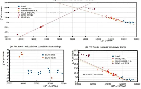
The (O −C) residuals from eq. 1 are plotted in Fig. 2a (lower left panel). It can
Figure 2. Top panel: The (O−C) diagram including timings from 1966 to 2016; (O−C) is the residual between the observed times of extrema and those computed from eq. 1; Lower left panel: The
Table 2 Ephemeris timings from NASAcam light curves.
Cycle HJD (O−C) Quality UT date
−2400000 min min
4464.55 57436.5893 −5.3 3.6 02/18/16†
4462.00 57435.6860 −5.1 2.9 02/17/16
†
4050.00 57289.7173 5.8 6.9 09/25/15†
4016.55 57277.8653 5.0 5.9 09/12/15 3977.00 57263.8468 −2.5 2.3 08/29/15
3403.55 57060.6535 −22.0 4.2 02/07/15∗
3401.00 57059.7524 −18.6 4.4 02/06/15
∗,† 3144.55 56968.9019 −0.4 3.3 11/06/14
3144.00 56968.7103 4.3 5.7 11/06/14 3015.00 56923.0091 11.4 1.8 09/23/14†
2221.55 56641.8701 −4.1 5.2 12/15/13
2221.00 56641.6785 0.6 5.0 12/15/13 1996.00 56561.9529 −7.4 7.2 09/26/13
1995.55 56561.7970 −2.3 3.9 09/26/13
1298.00 56314.6468 −2.9 1.8 01/22/13
1238.55 56293.5867 3.5 2.2 01/01/13 997.00 56208.0029 2.6 ∗∗ 10/08/12
979.55 56201.8135 −6.0 ∗∗ 10/01/12
931.00 56184.6200 4.9 ∗∗ 09/14/12
355.00 55980.5720 55.7 ∗∗ 02/23/12∗
237.00 55938.7628 55.0 2.1 01/11/12∗
236.55 55938.6030 55.5 3.6 01/10/12∗
234.00 55937.7040 61.0 6.9 01/10/12∗
0.55 55854.9807 48.5 4.7 10/20/11∗
0.00 55854.7853 46.8 4.0 10/20/11∗
−164.00 55796.6780 46.4
∗∗ 08/23/11∗
−212.00 55779.6710 46.3 ∗∗ 08/06/11∗
†timing derived by fitting template from 9/26/2013 (see text). ∗not used in fit for eq. 1, which was used to compute (O
−C).
∗∗used only B measures: 10/08/12 and 10/01/12 used one night each; 9/14/12 combined 2 nights; 2/23/12
com-bined 8 nights; 8/23/11 and 8/06/11 comcom-bined 3 nights each.
3.2 Ephemeris for the timings from survey data
To investigate the period change and extend the ephemeris back in time, we extracted timings from the archival survey datasets shown in Table 1, extending back to 2004, and they confirm that the period indeed had been different before 2011. After doing this we discovered timings made by Vandenbroere & Salmon (2009), which exhibit the same period as our survey results, thus verifying the period change. The ephemeris for the years 2004-2011 which we derive from those timings is
HJDmax = 2455854.763(6) + 0.3542890(1)E, (2)
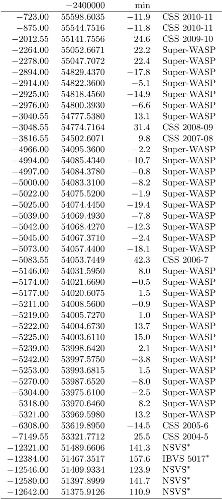
and the RMS residual from that fit is then 15.8 minutes. This is compatible with an estimate of the precision of the survey timings, and is consistent with Vandenbroere & Salmon (2009), the RMS of which is 14.4 minutes. Fig. 2b (lower right panel) shows the (O−C) residuals (still based on eq. 1) extended back to 1996.
Table 3 Ephemeris timings from survey light curves.
Cycle HJD (O−C) Source
−2400000 min
−723.00 55598.6035 −11.9 CSS 2010-11 −875.00 55544.7516 −11.8 CSS 2010-11
−2012.55 55141.7556 24.6 CSS 2009-10 −2264.00 55052.6671 22.2 Super-WASP
−2278.00 55047.7072 22.4 Super-WASP −2894.00 54829.4370 −17.8 Super-WASP
−2914.00 54822.3600 −5.1 Super-WASP −2925.00 54818.4560 −14.9 Super-WASP
−2976.00 54800.3930 −6.6 Super-WASP −3040.55 54777.5380 13.1 Super-WASP −3048.55 54774.7164 31.4 CSS 2008-09
−3816.55 54502.6071 9.8 CSS 2007-08 −4966.00 54095.3600 −2.2 Super-WASP
−4994.00 54085.4340 −10.7 Super-WASP −4997.00 54084.3780 −0.8 Super-WASP
−5000.00 54083.3100 −8.2 Super-WASP −5022.00 54075.5200 −1.9 Super-WASP
−5025.00 54074.4450 −19.4 Super-WASP −5039.00 54069.4930 −7.8 Super-WASP −5042.00 54068.4270 −12.3 Super-WASP
−5045.00 54067.3710 −2.4 Super-WASP −5073.00 54057.4400 −18.1 Super-WASP
−5083.55 54053.7449 42.3 CSS 2006-7 −5146.00 54031.5950 8.0 Super-WASP
−5174.00 54021.6690 −0.5 Super-WASP −5177.00 54020.6075 1.5 Super-WASP −5211.00 54008.5600 −0.9 Super-WASP
−5219.00 54005.7270 1.0 Super-WASP −5222.00 54004.6730 13.7 Super-WASP
−5225.00 54003.6110 15.0 Super-WASP −5239.00 53998.6420 2.1 Super-WASP
−5242.00 53997.5750 −3.8 Super-WASP −5253.00 53993.6815 1.5 Super-WASP
−5270.00 53987.6520 −8.0 Super-WASP −5304.00 53975.6100 −2.5 Super-WASP −5318.00 53970.6460 −8.2 Super-WASP
−5321.00 53969.5980 13.2 Super-WASP −6308.00 53619.8950 −14.5 CSS 2005-6
−7149.55 53321.7712 25.5 CSS 2004-5 −12321.00 51489.6606 141.3 NSVS∗ −12384.00 51467.3517 157.6 IBVS 5017
∗
−12546.00 51409.9334 123.9 NSVS∗ −12580.00 51397.8999 141.7 NSVS
∗
−12642.00 51375.9126 110.9 NSVS∗
∗not used in fit for eq. 2, which was used to compute (O
−C).
3.3 Ephemeris for timings between 1996 and 2001
There is a gap in the available timings of about three years before 2004 but the NSVS allows some estimates between 1996 and 2001, as well as five timings taken from IBVS between 1996 and 1999. As shown at the end of Table 3, these timings are inconsistent with the ephemeris given in eq. 2, the residuals being over two hours. Therefore there must have been another period change within that gap.
after, and is represented by
HJDmax = 2455855.00(4) + 0.354301(3)E. (3)
[image:8.595.168.429.196.341.2]Table 4 shows the timings and the residuals, which have an RMS of 16.1 min. The next earlier timing, given in the last line of that table, has a residual of over three hours, showing that another period change must have occurred.
Table 4 Ephemeris timings between 1996 and 2000.
Cycle HJD (O−C) Source
−2400000 min
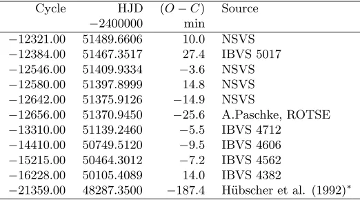
−12321.00 51489.6606 10.0 NSVS −12384.00 51467.3517 27.4 IBVS 5017
−12546.00 51409.9334 −3.6 NSVS −12580.00 51397.8999 14.8 NSVS
−12642.00 51375.9126 −14.9 NSVS
−12656.00 51370.9450 −25.6 A.Paschke, ROTSE
−13310.00 51139.2460 −5.5 IBVS 4712 −14410.00 50749.5120 −9.5 IBVS 4606
−15215.00 50464.3012 −7.2 IBVS 4562 −16228.00 50105.4089 14.0 IBVS 4382
−21359.00 48287.3500 −187.4 H¨ubscher et al. (1992)∗
∗not used in fit for eq. 3, which was used to compute (O
−C).
3.4 Ephemeris for timings between 1972 and 1996
Before 1996, timings are sparse back to the discovery paper, but we managed to find an ephemeris which fit well the ones between 1970 and 1991, which is
HJDmax= 2455855.73(2) + 0.3543421(5)E. (4)
The RMS residual of those timings from this ephemeris is 12.7 minutes, lower than we have any right to expect. Thus, contrary to several published suggestions, the period seems to have been constant for over 20 years. Fig. 2c (upper panel) shows the (O−C)
residuals (still based on eq. 1) extended back to 1966. Table 5 contains the timings and residuals from this even earlier epoch.
3.5 Ephemeris for timings before 1972
When Detre (1937) discovered RW Ari to be variable, he derived an alias (0.2614151 days) to the true period. Though his dataset is not very good by today’s standards, being photographic magnitudes, it is useful in determining the ephemeris at that early epoch. Notni (1962) observed the star photoelectrically in 1959, and published a new ephemeris with the approximately correct period of 0.3543184 days. He promised to publish his actual data, but that evidently was never done. Todoran (1988) found a period compatible with the data of Detre, Wi´sniewsi, and Penston of 0.3543145 days, but this is incompatible with Notni’s period.
We find that Todoran probably made a cycle count error by adding one cycle to the gap between Detre and Wi´sniewski’s data. We have derived a new ephemeris for those years:
Table 5 Ephemeris timings between 1970 and 1991.
Cycle HJD (O−C) Source
−2400000 min
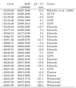
−21359.00 48287.3500 15.2 H¨ubscher et al. (1992)
−35128.00 43408.4040 2.1 GCVS −35139.00 43404.5004 −6.3 GS79
−35142.00 43403.4460 6.1 GS79 −35156.00 43398.4814 0.7 GS79
−35166.00 43394.9280 −13.7 Edwards −35177.55 43390.8500 7.4 Edwards
−35948.55 43117.6530 8.5 Edwards −35962.55 43112.6900 5.3 Edwards −35971.00 43109.6770 −21.7 Edwards
−36086.55 43068.7620 −5.2 Edwards −36098.00 43064.6800 −15.3 Edwards
−36100.55 43063.7960 12.9 Edwards −36166.00 43040.5900 −7.7 GS79
−36175.00 43037.4150 12.5 GS79 −36185.00 43033.8550 −11.3 Edwards
−36230.00 43017.9050 −18.0 Edwards −36233.00 43016.8430 −16.5 Edwards −36251.00 43010.4820 8.2 GS79
−42163.00 40915.6190 19.4 Penston −42165.00 40914.9090 17.5 Penston
−46224.00 39476.7173 137.1 Wi´sniewski
∗
−46227.00 39475.6592 144.1 Wi´sniewski∗ −46401.00 39413.9913 126.3 Wi´sniewski
∗
∗not used in fit for eq. 4, which was used to compute (O
−C).
We can use Notni’s ephemeris to estimate a timing for his epoch:
HJDmax= 2428183.324 + 0.3543184×24501 = 2436864.4791 (6)
which corresponds to UT 23 Oct, 1959 23:30. Note this is NOT an actual timing from Notni, but a time which fits his ephemeris, and is therefore possible. The phase of this time, based on Todoran’s ephemeris, is 0.325, which is incompatible. The phase derived from eq. 5 is also incompatible, being 0.561. Without finding Notni’s actual data, we cannot decide whether this indicates another period change, or some problem with that data.
Lastly, we note the excellent fit of Penston’s data to eq. 5, but the large residuals of about 18 minutes based on eq. 4 suggest that the period change in 1972 took place some-what after Penston recorded her data. It is possible that the Harvard Plate Collection2 could shed light on the behavior of the star in these gaps, but plates from that part of the sky have not yet been scanned.
It is clear that the star has changed its period at least three and possibly four or five times since its discovery, and it is clear that anomalous (but not seemingly periodic) excursions in timings occur, which means the star should be monitored in the future, to extend and verify these behaviors.
2
4
The Light Curve
On UT 20 Oct, 2011 we used NASAcam at Lowell Observatory to obtain light curves of RW Ari in B, V, R, and I filters. The images were processed using IRAF3 for overscan, zero, and flat field corrections. Magnitudes were extracted with IRAF task qphot, and
[image:10.595.141.458.236.305.2]corrected approximately to standard values by using the average of the comparison stars listed in Table 6. The magnitudes of the comparison stars were measured by observing Landolt field 92 on UT 26 Sept, 2013, to produce a final light curve, shown in Fig. 3 for the V filter.
Table 6 Stars used from NASACam images.
Object Purpose B magnitude V magnitude Comments RW Ari Target 12.40-12.96 12.06-12.48 RA 2h
16m
03s.
7 dec +17◦31′04′′
BD +16 262 Comp 1 11.72 11.01 22s
W and 22′′S
BD +15 264 Comp 2 11.63 10.96 13s
E and 3′N
Un-named Check 12.65 12.03 1s.
8 E and 6′′S
The light curve shows a broad maximum, a slow decline in brightness, a rather narrower minimum at phase 0.55, and a more rapid rise to maximum. On the rising branch the star remains constant for about 25 minutes (phase 0.815 to 0.865), thus it exhibits a stillstand. The check star used was the companion star about 1.8s to the east, which is a mid-F star of similar color to RW Ari, and its magnitude is shown also in Fig. 3.
The lower panel shows the (B−V) color, which is bluest at phase 0.00 when the star is
brightest, and reddest at phase 0.55 when the star is faintest. Light curves at additional 13 epochs over the next five years show no differences from the one presented in Fig. 3, after being corrected to consistent phase; no measures in B filter or in Super-WASP data show any deviation. The light curve appears to be quite repeatable over at least 10 years.
5
Radial Velocities
Spectra were taken with the Boller and Chivens spectrograph on the Bok 2.3-m telescope at Steward Observatory on Kitt Peak AZ during 2012-2014. We used this instrument configured with the 832 lines/mm grating in second order, which yields a dispersion of 0.72 ˚A/pix (50 km s−1), and a 1.5 arcsec entrance slit, which gives a resolution of 0.88˚A.
The camera was the Loral thinned, back-illuminated 1200×800 chip binned 1×2, so the
effective 2-pixel resolution was undersampled at 1.44˚A, or 100 km s−1 over the region
3850-4700˚A. The exposure time of 10 minutes yielded a S/N of about 100. Six HeAr comparison spectra were taken before and after each pair of target spectra, and averaged, for wavelength calibration.
The spectra were reduced with IRAF, and task fxcor was used to derive radial
ve-locities by cross-correlating with the template spectrum (Image 0067 from 4 Nov 2014), which was of HD222368 (an F7V star with heliocentric radial velocity +5.95 km s−1).
Ta-ble 7 gives the image number, HJD (minus 2400000), phase based on the listed ephemeris, the radial velocity, and the formal error from fxcor. Fig. 4 shows the resulting radial
velocity curve; spectra from UT 11 Jan, 2012 were included to help fill the gap near phase
3
Figure 3. TheV and (B−V) light curves derived from images obtained on October 20, 2011 with NASAcam.
0.80 when the velocity was rapidly decreasing. The radial velocities from Jeffery et al. (2007) are also plotted, but with their phase updated. The individual spectra are avail-able in a web database through the IBVS website as a gzipped tar archive6180.tar.gz.) When used only with hydrogen lines (Hγ, Hδ, Hǫand Hζ), the velocities were consistently 7 km s−1 redward, and when used only with lines other than hydrogen, were 3 km s−1
blueward of the tabulated values.
The median heliocentric velocity is−47.5 km s−1, which would induce a period change
of +4.8 seconds due to Doppler shift, as suggested by Davies et al. (2014).
Along with the spectra used for Table 7, we obtained radial velocities on two additional nights in 2012 and two in December 2013, but these velocities appeared to be anomalous, in that there were jumps in the velocity curve which would not make sense for a single star. It is remotely possible that this is evidence of a light travel time effect in a binary system, but the orbit would need to be highly elliptical and oriented in a special way to our line of sight.
The final problem with radial velocities of this star is the measurements of Abt & Wi´sniewski (1972), who found a discrepancy of 35 km s−1 on two nights chosen to have
the same pulsation phase, but different orbital phases. However, there was a period change in the pulsation before the spectra were obtained, and in fact, the conditions on phase were not met (see section 3). Even so, the second measure is given by them as
−11 km s−1, which is much bluer than any we obtained. One possibility was that the
companion star was inadvertently measured, which has roughly this velocity.
Figure 4. The radial velocity curve derived from spectra from UT 3 Nov, 2014 and UT 12 Jan, 2012. The four radial velocities above−20 km s−1 are for the companion star, which while not an RV
standard, appears to have constant velocity.
We reduced the spectra twice, once using Abt’s eight comparison lines and five stellar lines (Hγ, Hδ, Ca II K, Hζ, and Hǫ), and once using all the lines in both the comparison and stellar spectra (over 50 of each). We used IRAF task rvid to derive velocities, and
both methods agree well with the photographic measurements. Even the companion’s ve-locity agrees with the ones we measured here. Thus we are unable to find any explanation for the anomaly in the spectra themselves.
6
Conclusions
Although RW Ari has long been suspected of being in an eclipsing binary system, we find that this is almost certainly not the case. Except under extremely unusual circumstances, an eclipse would have been seen by now, with the plethora of photometric measurements that have been made of the star.
The star remains an interesting object in itself. It has changed its period abruptly several times since being discovered, at least around 1968, 1994, 2002, and 2011. It also exhibits anomalous behavior on a short timescale, where for a few nights to a few months, the light curve appears shifted in phase from the normal ephemeris before and after. One possible explanation for this phenomenon was suggested by Learned et al. (2008), ie that an advanced civilization could modulate pulsating star phase as a means of communication. If this is the explanation for RW Ari, we have no clue what message we are being sent.
Table 7 Measured radial velocities for RW Ari.
Image HJD (mid) phase∗ RV helio uncertainty Comments
−2400000 km s
−1
km s−1
3 Nov 2014
21 56965.6185 0.274 −49.2 4.9
22 56965.6265 0.297 −51.3 4.8
35 56965.6432 0.344 −49.3 4.7
36 56965.6503 0.364 −47.4 4.8
37 56965.6575 0.384 −49.5 4.6
38 56965.6665 0.410 −15.8 1.4 companion
51 56965.6798 0.447 −46.7 4.5
52 56965.6868 0.467 −45.5 4.3
53 56965.6939 0.487 −42.9 4.2
54 56965.7010 0.507 −35.3 3.8
67 56965.7145 0.545 −41.2 4.3
68 56965.7215 0.565 −41.6 4.4
69 56965.7286 0.585 −37.6 3.9
70 56965.7357 0.605 −35.5 4.2
83 56965.7501 0.646 −14.2 1.5 companion
96 56965.7650 0.688 −34.5 4.4
97 56965.7721 0.708 −36.1 4.4
110 56965.7883 0.753 −37.8 4.7
111 56965.7954 0.773 −36.3 4.7
143 56965.8301 0.871 −57.2 5.1
144 56965.8372 0.891 −58.5 5.1
157 56965.8505 0.929 −59.9 5.1
158 56965.8575 0.949 −62.2 5.3
171 56965.8722 0.990 −61.1 5.2
172 56965.8793 0.010 −61.0 5.1
173 56965.8863 0.030 −61.6 5.0
174 56965.8934 0.050 −59.5 5.1
187 56965.9071 0.089 −15.2 1.4 companion
188 56965.9160 0.114 −56.1 5.4
201 56965.9296 0.152 −57.1 4.9
202 56965.9367 0.172 −54.6 5.1
11 Jan 2012
7 55937.5900 0.678 −32.2 5.4
8 55937.5976 0.700 −29.9 5.4
21 55937.6122 0.741 −39.0 5.4
22 55937.6212 0.766 −16.2 3.7 companion
35 55937.6358 0.807 −44.1 5.4
36 55937.6429 0.828 −49.7 5.3
49 55937.6587 0.872 −62.5 5.3
50 55937.6658 0.892 −66.4 5.3
∗The phases for 3 November, 2014 were calculated from the light curve from three nights later, ie phase 0 = HJD
56968.7103. The phases for 11 January, 2012 were calculated from the light curve from the same night, ie phase 0 = HJD 55937.7040. ‘companion’ indicates a spectrum of the photometric check star.
could produce period changes in RR Lyr stars such as we observe for RW Ari.
The light curve of RW Ari is rather typical of an RRc star, roughly sinusoidal, but with a steeper rise in brightness than fall. It shows a stillstand of about a half hour during the rise time. Even though the period changes in strange ways, the light curve repeats itself quite well.
when the velocity appears quite different than expected. While this could be a problem with the observations (A-type stars are notably difficult to measure velocities for), it could also indicate a long-period binary orbit, but that would require a very specific orientation of the orbit.
As in most similar studies, more work needs to be done on the star, in particular, con-tinued monitoring for period changes and erratic behavior of the pulsation cycle. Future sky surveys could prove extremely valuable in this endeavor.
Acknowledgements: We would like to thank Lowell Observatory for making time avail-able on their 0.8-m telescope, and Steward Observatory for time allocated on the Bok 2.2-m telescope. We especially appreciate Robert West’s effort to supply us with Super-WASP photometry, which was essential for the work done here. We thank Helmut Abt for loaning his spectra from Kitt Peak. We benefited from discussions with Eckhart Spalding, Horace Smith, and Sebastian Otero, as well as Jacqueline Vandenbroere and Chris Sterken. This research has made use of the SIMBAD database, operated at CDS, Strasbourg, France.
References:
Abt, H. A., Wi´sniewski, W. Z., 1972, IBVS, 697
Agerer, F., Dahm, M., H¨ubscher, J., 1999,IBVS,4712
Agerer, F., Dahm, M., H¨ubscher, J., 2001,IBVS,5017
Agerer, F., H¨ubscher, J., 1996, IBVS,4382
Agerer, F., H¨ubscher, J., 1998, IBVS,4562
Agerer, F., H¨ubscher, J., 1998, IBVS,4606
Bookmyer, B. B. et al., 1977, RMxAA,2, 235 Buie, M. W., 2010, Adv. in Astron., AID:130172 Davies, G. R. et al., 2014, MNRAS, 445, L94 Detre, L., 1937, AN, 262, 81
Drake, A. J., et al., 2014, ApJS,213, 9
Edwards, D. A., 1978, A photometric investigation of the variable RW Arietis, master thesis, University of Texas, Austin, USA
Goranskij, V. P., Shugarov, S. Y., 1979, Peremennye Zvezdy,21, 211 (GS79) H¨ubscher, J., Agerer, F., Mundry, E., 1992, BAV Mitt., 60, 1
Jeffery, E. J. et al., 2007,ApJS, 171, 512
Kwee, K. K., van Woerden H. 1956, BAN, 12, 327
Learned, J. G., Kudritzki, R-P., Pakvasa1, S., Zee A. 2008, arXiv:0809.0339 Liska, J., Skarka, M., Hajkova, P., & Auer, R. F. 2016, arXiv:1601.03082 Mankiewicz, L., et al., 2014, RMxAC, 45, 7
Notni, P., 1962, Mitteilungen ¨uber Ver¨anderliche Sterne,1, 667 Odell, A. P., 2012, A&A, 544, A28
Pojmanski, G., 2002, AcA, 52, 397
Pollacco, D. L. et al., 2006,PASP,118, 1407 Sweigart, A. V. & Renzini, A., 1979, A&A,71, 66 Todoran, I., 1988, IBVS, 3149
Vandenbroere, J. & Salmon, G., 2009, GEOS Circular RR, 38