Nonlinear Observer-Based Tracking Control Using
Piecewise Multi-Linear Models
Tadanari Taniguchi and Michio Sugeno
Abstract—This paper proposes a nonlinear observer-based tracking controller design using piecewise multi-linear models. The controller is based on feedback and observer linearizations. The piecewise model is a nonlinear approximation and fully parametric. Feedback linearization is an effective method to stabilize nonlinear systems. However the stabilizing conditions are conservative. Further, observer linearization conditions are more conservative than feedback one. There are not many nonlinear systems to which these methods can apply. This paper shows the proposed piecewise multi-linear controller can be applied to a wider class of nonlinear systems. Example is shown to confirm the feasibility of our proposals by computer simulation.
Index Terms—observer-based control, nonlinear control, feedback linearization, tracking control, piecewise system.
I. INTRODUCTION
P
Iecewise linear (PL) systems which are fully paramet-ric have been intensively studied in connection with nonlinear systems [1], [2], [3], [4]. We are interested in the parametric piecewise approximation of nonlinear control systems based on the original idea of PL approximation. The PL approximation has general approximation capability for nonlinear functions with a given precision.PML approximation [5] also has general approximation capability for nonlinear functions with a given precision. We note that a bilinear function as a basis of PML approxi-mation is, as a nonlinear function, the second simplest one after a linear function. The PML model has the following features. 1) The PML model is derived from fuzzy if-then rules with singleton consequents. 2) It is built on piecewise hyper-cubes partitioned in the state space. 3) It has general approximation capability for nonlinear systems. 4) It is a piecewise nonlinear model, the second simplest after a PL model. 5) It is continuous and fully parametric. So far we have shown the necessary and sufficient conditions for the stability of PML systems with respect to Lyapunov functions in the two dimensional case [6] where membership functions are fully taken into account. However, since the stabilizing conditions are represented by bilinear matrix inequalities (BMIs) [7], it requires a long computing time to obtain a stabilizing controller. To overcome the difficulty, we derived the stabilizing conditions [8] based on a full-state feedback linearization approaches. Although the PML controllers are simpler than the conventional feedback linearization con-troller, the control performance based on PML model is the same as the conventional one.
This paper deals with an observer-based tracking controller design for nonlinear systems via observer linearization.
Manuscript received December 25, 2018; revised January 10, 2019. T. Taniguchi is with IT Education Center, Tokai University, Hiratsuka, Kanagawa, 2591292 Japan email:[email protected]
M. Sugeno is with Tokyo Institute of Technology.
We proposed some observer design methods for piecewise systems in [9], [10], [11]. The paper [11] dealt with the necessary and sufficient conditions for observer linearization and showed the PML model based linearized observer could be applied to a wider system than the conventional one. However it is difficult to design the observer-based control system via observer linearization because the control system is not robust to modeling errors and perturbations. We pro-posed a robust observer-based PML controller design [12] for nonlinear systems using a robust PML controller [13]. This paper proposes a nonlinear observer-based tracking controller using piecewise multi-linear models. Further, we apply the proposed methods to TORA (Translational Oscillator with Rotating Actuator) system, which is one of the benchmark problem for nonlinear control. Example is shown to confirm the feasibility of our proposals by computer simulation.
II. CANONICALFORMS OFPIECEWISEMULTI-LINEAR
MODELS
A. Open-Loop Systems
In this section, we introduce PML models suggested in [5]. We deal with the two-dimensional case without loss of generality. We consider a two-dimensional nonlinear system:
˙ x=f(x)
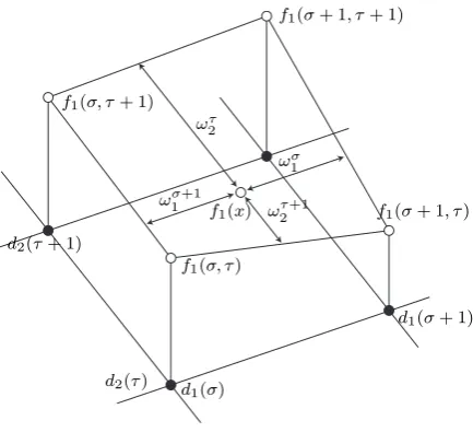
Define vectord(σ, τ)and rectangleRστ in two-dimensional space asd(σ, τ)≡(d1(σ), d2(τ))
T ,
Rστ ≡[d1(σ), d1(σ+ 1)]×[d2(τ), d2(τ+ 1)]. σ and τ are integers: −∞ < σ, τ < ∞ where d1(σ) < d1(σ+ 1), d2(τ)< d2(τ+ 1)andd(0,0)≡(d1(0), d2(0))T
(see Fig. 1). SuperscriptT denotes atransposeoperation. Forx= (x1, x2)∈Rστ, the PML system is expressed as
˙
x=fp(x) = σ+1 X
i=σ τ+1 X
j=τ
ωi1(x1)ω
j
2(x2)f(i, j),
x=
σ+1 X
i=σ τ+1 X
j=τ
ω1i(x1)ωj2(x2)d(i, j),
f(i, j) =f(d1(i), d2(j)), d(i, j) = [d1(i), d2(j)]T,
(1)
wheref(i, j)is the vertex of nonlinear systemx˙ =f(x),
ωσ1(x1) =
(d1(σ+ 1)−x1) (d1(σ+ 1)−d1(σ))
,
ωσ1+1(x1) =
(x1−d1(σ)) (d1(σ+ 1)−d1(σ))
,
ωτ2(x2) =
(d2(τ+ 1)−x2) (d2(τ+ 1)−d2(τ))
,
ωτ2+1(x2) =
(x2−d2(τ)) (d2(τ+ 1)−d2(τ))
and ωi
1(x1), ω
j
2(x2) ∈ [0, 1]. In the above, we assume f(0,0) = 0andd(0,0) = 0to guarantee x˙ = 0 forx= 0.
A key point in the system is that state variable xis also expressed by a convex combination of d(i, j) for ωi
1(x1)
andωj2(x2), just as in the case ofx˙. As seen in equation (2), x is located inside Rστ which is a rectangle: a hypercube in general. That is, the expression of x is polytopic with four vertices d(i, j). The model of x˙ =f(x) is built on a rectangle includingxin state space, it is also polytopic with four verticesf(i, j). We call this form of the canonical model (1) parametric expression.
B. Closed-Loop Systems
We consider a two-dimensional nonlinear control system.
( ˙
x=f(x) +g(x)u(x),
y=h(x). (3)
For x ∈ Rστ, the PML model (4) is constructed from a nonlinear system (3).
( ˙
x=fp(x) +gp(x)u(x),
y=hp(x),
(4)
where
fp(x) = σ+1 X
i=σ τ+1 X
j=τ
ω1i(x1)ω
j
2(x2)f(i, j),
gp(x) = σ+1 X
i=σ τ+1 X
j=τ
ω1i(x1)ωj2(x2)g(i, j),
hp(x) = σ+1 X
i=σ τ+1 X
j=τ
ω1i(x1)ω
j
2(x2)h(i, j),
x=
σ+1 X
i=σ τ+1 X
j=τ
ω1i(x1)ωj2(x2)d(i, j),
(5)
and f(i, j), g(i, j), h(i, j) and d(i, j) are vertices of the nonlinear system (3). The modeling procedure in regionRστ is as follows:
1) Assign verticesd(i, j)forx1=d1(σ),d1(σ+1),x2= d2(τ),d2(τ+ 1)of state vector x, then partition state
space into piecewise regions (see Fig. 1).
2) Compute verticesf(i, j),g(i, j)andh(i, j)in equation (5) by substituting values ofx1=d1(σ),d1(σ+1)and x2=d2(τ),d2(τ+1)into original nonlinear functions f(x),g(x) and h(x)in the system (3). Fig. 1 shows the expression off1(x)andx∈Rστ.
The overall PML model is obtained automatically when all vertices are assigned. Note that f(x), g(x)andh(x)in the PML model coincide with those in the original system at vertices of all regions. Due to lack of space,f(x),g(x),u(x), andh(x)are represented asf,g,u, andh, respectively.
III. REGULATOR ANDTRACKINGCONTROLLERDESIGNS FORPML SYSTEMS
A. Feedback Linearization
This section deals with the PML controller for nonlinear systems. Since the stabilizing conditions are represented by bilinear matrix inequalities (BMIs) [7], it requires a long computing time to obtain a stabilizing controller. To
d1(σ)
d1(σ+ 1)
d2(τ)
d2(τ+ 1)
f1(σ+ 1, τ)
f1(σ, τ)
f1(σ, τ+ 1)
f1(σ+ 1, τ+ 1)
ω1σ+1
ωσ1
ω2τ+1 ωτ
2
[image:2.595.328.545.50.253.2]f1(x)
Fig. 1. Piecewise region (f1(x) = Pσ+1i=σPτ+1j=τωi1ω2jf1(i, j), x ∈
Rστ)
overcome the difficulty, we derived the stabilizing conditions [14], [8] based on feedback linearization approaches.
We consider the PML system (4), where fp, gp and hp are assumed to be sufficiently smooth in a domainD⊂Rn. The mappings f : D → Rn and g : D → Rn are called vector fields on D. The time derivative of the output y is calculated until the inputuappears. Then the PML controller is obtained as
u(x) =α(x) +β(x)v, (6)
where
α(x) = −L
ρ fph LgpL
ρ−1
fp hp
, β(x) = 1
LgpL
ρ−1
fp hp .
The controller reduces the input-output map to y(ρ) = v,
which is a chain ofρintegrators. In this case, the integer ρ
is called the relative degree of the system.
In Section VI, we show the controller (6) based on PML model is simpler than the conventional feedback linearzing controller. Furthermore, we show the controller (6) can stabilize a wider region than the conventional one.
Definition 3.1: The PML system is said to have relative degreeρ,1≤ρ≤n, in a regionD0⊂D if
LgpL
i
fphp= 0, i= 0,1,· · · , ρ−2 LgpL
ρ−1
fp hp6= 0,
for all x ∈ D0. The feedback linearized system can be
formulated as
(˙
ξ=Aξ+Bv,
y=Cξ, (7)
whereξ∈ <ρ,
A=
0 1 0 · · · 0
0 0 1 . .. ... ..
. ... . .. . .. 0 0 0 · · · 0 1 0 0 · · · 0 0
, B=
0 0
.. .
0 1
, C=
1 0
.. .
0 0
T
The stabilizing linear controllerv=−Kξof the linearized system (7) can be obtained so that the transfer functionG= C(sI−A)−1B is Hurwitz. Due to lack of space, this paper
only deals with the relative degree ρ = n. This controller design can be applied to the PML system with the relative degreeρ≤n.
B. Tracking Control for PML Systems
We apply a tracking control [15] to nonlinear systems. Consider the following reference signal model
( ˙ xr=fr,
yr=hr.
(8)
The controller is designed to make the error signal et =
y−yr=hp−hr→0ast→ ∞. The time derivative of the errore is obtained as
˙
et=Lfphp−Lfrhr.
The time derivative is calculated until the input uappears. Then the PML controller is obtained as
ut(x) =αt(x) +βt(x)vt, (9) where
αt(x) =−
Lρf
php−L
ρ frhr LgpL
ρ−1
fp hp
, βt(x) =
1
LgpL
ρ−1
fp hp .
The controller reduces the input-output map to y(ρ) = v,
which is a chain of ρintegrators. In this case, the integerρ
is called the relative degree of the system.
IV. OBSERVERDESIGN FORPML SYSTEMS
A. Observer Linearization
This subsection deals with the observer linearization prob-lem [16]. If there exists a coordinate transformationζ=ϕ(x)
such that the system (4) can be transformed into the follow-ing system:
˙
ζ=Aoζ+k(y) +r(y)u
y=Coζ
with(Co, Ao) observable andk, r:< → <n then it would be possible to build a full order state observer [11]:
˙ˆ
ζ=Aoζˆ+k(y) +H(ˆy−y)
ˆ y=Coζ,ˆ where
Ao=
0 0 · · · 0 0 1 0 · · · 0 0
0 1 . .. ... ... ..
. . .. . .. 0 0 0 · · · 0 1 0
, Co=
0 0
.. .
0 1
T
,
andH is the observer gain. The estimation erroreo= ˆζ−ζ satisfies the linear differential equation
˙
eo=(Ao+HCo)e.
The estimation state isxˆ=ϕ−1( ˆζ). This problem is referred to as the observer linearization problem. The following
theorem gives a necessary and sufficient condition for the solution of the observer linearization problem.
Theorem 4.1: The observer linearization problem [16] is solvable if and only if there exists the neighborhoodV of an initial conditionx(0)satisfies the following two conditions.
C1: dimspan{dh, dLfh, . . . , dLnf−1h}
=n, ∀x∈V.
C2: [adi fτ, ad
j fτ] = 0,
0≤i≤n−1,0≤j ≤n−1,x∈V. The vector fieldτ satisfies
dh, dLfh, . . . , dLnf−1h
T
τ = 0, . . . ,1T .
If the nonlinear system (3) is observer linearizable there ex-ists a coordinate transformationϕ(x) satisfies the following condition.
L(−1)j−1adj−1
f τ
ϕi(x) =
( 0, i6=j
1, i=j (10)
A coordinate transformation can be constructed as ζ = ϕ(x) = (ϕ1(x), ϕ2(x), . . . , ϕn(x))T.
B. Observer Based Controller Design
We consider observer-based PML controllers [12]. Substi-tuting the estimation state xˆ = ϕ−1( ˆζ) into the controller
(6), the observer-based PML controller can be designed as
u(ˆx) =α(ˆx) +β(ˆx)v
wherev=−Kξˆandξˆ= (h(ˆx), Lfh(ˆx), . . . , L ρ−1
f h(ˆx)) T. We propose an observer-based PML tracking controller. Substituting the estimation state xˆ = ϕ−1( ˆζ) into the controller (9), the controller can be designed as
ut(ˆx) =αt(ˆx) +βt(ˆx)vt
where vt = −Fξˆr and ξˆt = (h(ˆx) − hr, Lfh(ˆx) −
Lfrhr, . . . , L
ρ−1
f h(ˆx)−L ρ−1
fr hr)
T.
V. TORA SYSTEM
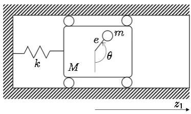
The TORA (Translational Oscillator with Rotating Ac-tuator) system [17] has a cart of mass M connected to a wall with a linear spring (constantk). The cart can oscillate without friction in the horizontal plane. A rotating massm
[image:3.595.332.519.655.766.2]in the cart is actuated by a motor. The mass is eccentric with a radius of eccentricityeand can be imagined to be a point mass mounted on a massless rotor. The rotating motion of the massmcontrols the oscillation of the cart. The motor torque is the control variable. The dynamics of TORA system is
˙ z1=z2
˙ z2=
−z1+εz24sinz3 1−ε2cos2z
3
− −εcosz3
1−ε2cos2z 3
v
˙ z3=z4
˙ z4=
1 1−ε2cos2z
3
εcosz3 z1−εz24sinz3
+v
y=z1,
(11) where z1 and z2 are the position and velocity of the cart. z3=θandz4= ˙θ are the angle and angular velocity of the
rotor. The parameterεdepends on the eccentricityeand the masses M andm.v andy are the control input and output. The TORA system dynamics has many nonlinear terms. We consider the new variables:
x1=z1+εsinz3
x2=z2+εz4cosz3
u=εcosz3(x1−εsinz3(1 +z 2 4)) +v 1−ε2cos2z
3
Substituting the variables x1,x2 andu into TORA system
(11), we obtain
˙
x=f+gu=
x2
−x1+εsinx3 x4
0
+
0 0 0 1
u
y=h=x1,
(12)
wherex∈R4,y∈R. In the paper, we consider the system (12) as TORA system.
VI. PML MODEL-BASEDCONTROLS FORTORA
SYSTEM
A. PML Model
We construct the PML model [18] of TORA system (12). The state variable x is divided by m1×m2×m3 ×m4
vertices,
x1∈{d1(1), . . . , d1(m1)}, x2∈ {d2(1), . . . , d2(m2)},
x3∈{d3(1), . . . , d3(m3)}, x4∈ {d4(1), . . . , d4(m4)}.
The PML model is expressed as
( ˙
x=fp+gpu
y=hp=x1,
(13)
wherex∈Rσ1σ2σ3σ4,
fp= σ1+1
X
i1=σ1 σ2+1
X
i2=σ2 σ3+1
X
i3=σ3 σ4+1
X
i4=σ4
ωi1
1 (x1)ωi22(x2)ω3i3(x3)ωi44(x4)
× d2(i2) −d1(i1) +εsind3(i3) d4(i4) 0 T
,
gp= 0 0 0 1
T ,
ωσj
j (xj) = (dj(σj+ 1)−xj)/(dj(σj+ 1)−dj(σj)),
ωσj+1
1 (xj) = (xj−dj(σj))/(dj(σj+ 1)−dj(σj)),
j= 1, . . . ,4.
The model is found to be fully parametric and the internal model dynamics is described by multi-linear interpolation of the vertices:d1(i1),d2(i2),d3(i3) andd4(i4). The PML
model can be represented by a lookup table (LUT).
Note that trigonometric functions of TORA system (12) are smooth functions and are of classC∞. The PML models are not of class C∞. In TORA system control, we have to calculate the fourth derivatives of the outputy. Therefore the derivative PML models lose some dynamics. However the PML model based control for TORA system can be applied to a wider region than the conventional one.
Note that there are some modeling errors because the PML model is a nonlinear approximation. In proposed method the verticesdi(j)of an arbitrary number can be set on arbitrary position of the state space. Therefore it is easily possible to adjust the approximated error.
B. Regulators
1) Feedback Linearization of Original Nonlinear System: We design the controller of TORA system (12) via the exact feedback linearization [16]. We calculate the time derivatives of the outputy until the inputuappears. Then the feedback linearizing controller is obtained as
u=−L 4
fh
LgL3fh
+ 1
LgL3fh
v. (14)
The Lie derivatives are calculated as
Lfh=x2, L2fh=−x1+εsinx3, L3fh=−x2+εx4cosx3,
L4fh=x1−εsinx3−εx42sinx3, LgL3fh=εcosx3.
In equation (14),v is the linear controller for the linearized system:
˙
ξ=Aξ+Bv
y=Cξ,
ξ=(h, Lfh, L2fh, L
3
fh) T,
A=
0 1 0 0
0 0 1 0
0 0 0 1
0 0 0 0
, B=
0 0 0 1
, C=
1 0 0 0
T
. (15)
However the controller (14) is only well defined at−π/2< x3 < π/2 because the denominator of the controller is LgL3fh = εcosx3. Hence the rotor of TORA system can
only be rotated at−π/2< θ < π/2.
2) Feedback Linearization of PML System: The time derivative of the outputy=x1 has to been calculated until
the inputuappears. Then the PML controller [18] of (13) is designed as
u= −L 4
fphp LgpL
3
fphp
+ v
LgpL 3
fphp
(16)
The Lie derivatives are calculated as
Lfphp=x2, L 2
fphp=−x1+
σ3+1
X
i3=σ3
ωi3
3(x3)εsind3(i3),
L3fphp=−x2+
ε(sind3(σ3+ 1)−sind3(σ3)) d3(σ3+ 1)−d3(σ3)
x4,
L4f
php=x1−
σ3+1
X
i3=σ3
ωi3
3(x3)εsind3(i3),
LgL3fphp=
In equation (16), v = −Kξ is the linear controller of the linear system:
˙
ξ=Aξ+Bv,
y=Cξ,
ξ=(hp, Lfphp, L 2
fphp, L 3
fphp)
T
The matrixAand the vectorsB andCare the same as (15). Iffs(i)6=fs(i+ 1) andd3(i)6=d3(i+ 1),i= 1, . . . , m,
there exists a controller (16)u of TORA system (13) since
det(LgpL 3
fphp) 6= 0. Thus we have to construct the PML
model of TORA system such that fs(i) 6= fs(i+ 1) and
d3(i)6=d3(i+ 1), wherei= 1, . . . , m. Note that the PML
model based controller (16) can be applied to a wider region than the conventional feedback linearized controller.
C. Tracking Control
We design the tracking controller of TORA system using PML model. Consider the following reference signal model (8). The controller is designed to make the error signalet=
y−yr=hp−hr→0ast→ ∞. The time derivative of the errore is obtained as
˙
et=Lfphp−Lfrhr.
The time derivative is calculated until the input uappears. Then the PML controller is obtained as
ut(x) =αt(x) +βt(x)vt, (17)
where
αt(x) =−
L4f php−L
4
frhr LgpL
3
fphp
, βt(x) =
1 LgpL 3
fphp .
In equation (16), vt=−F ξr is the linear controller of the linear system:
˙
ξr=Aξr+Bν,
y=Cξr,
ξr=
hp−hr
Lfphp−Lfrhr L2
fphp−L 2
frhr L3
fphp−L 3
frhr
The matrixAand the vectorsB andCare the same as (15).
D. Observers
1) Observer Design of Original Nonlinear System: C1 of Theorem 4.1 is calculated for the original nonlinear system (12).
det dhT, dL
fhT, . . . , dLnf−1hT T
=ε2cos2x3
From this result the above matrix is not linear independence atx3=±π/2. One of the condition C2 is calculated for the
original nonlinear model as follows:
ad0fτ, ad
3
fτ
= 2 sinx3 ε2cos3x 3
The above equation is equal to 0 atx3= 0and the equation
cannot be defined at x3 = ±π/2. Therefore the nonlinear
system (12) is not observer linearizable.
2) Observer Design [11] of PML System: C1 of Theorem 4.1 is calculated for the PML system (13).
det dhT, dLfhT, . . . , dLnf−1h TT
=ε6= 0.
C2 of Theorem 4.1 is also calculated for the original nonlin-ear system (13).
[adifτ, adjfτ] = 0,
where0 ≤i ≤3, 0 ≤j ≤3, and τ = 0 0 0 1/εT
. Therefore the PML system (13) is an observer linearizable. From the condition (10), the coordinate transformation vector is calculated asϕ(x) = εx4 εx3 x2 x1
T
.
E. Observer-Based Tracking Control
We derive an observer-based PML tracking controller for TORA system. Substituting the estimation statexˆ=ϕ−1( ˆζ)
into the controller (17), the controller can be designed as
ut(ˆx) =αt(ˆx) +βt(ˆx)vt (18)
where vt = −Fξˆr and ξˆt = (h(ˆx) − hr, Lfph(ˆx) − Lfrhr, . . . , L
ρ−1
fp h(ˆx)−L
ρ−1
fr hr)
T.
VII. SIMULATIONRESULT
The observer-based PML controller (18) is applied to TORA system (12) in computer simulations. In the simu-lation, the state variables x1, x2, x3, x4 of TORA system
are divided by the following vertices.
x1∈{−2.0, 0, 2.0}, x2∈ {−2.0, 0, 2.0},
x3∈{−π,−7π/8, . . . , π}, x4∈ {−2.0, 0, 2.0}
The parameter ε is 0.5 and the initial condition is x(0) = (0.5, 0, 0, 0)T. We consider the following reference signal model:
( ˙
xr=arcost,
yr=hr=xr,
where ar = 0.2. We use the feedback gain F =
(1.000, 3.078, 4.236, 3.078) such that the linearized control system is stable and the observer gain H = (10.00, 25.09, 26.47, 12.37)T such that the observer system is stable.
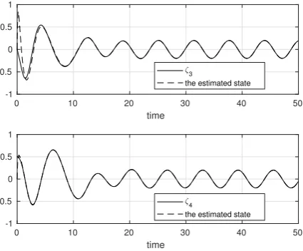
Figs. 3, 4, and 5 show the simulation results using the observer-based tracking controller (18). The controller (18) stabilize the TORA system (12) with the estimation error
eo= ˆζ−ζand the tracking error et=y−yr. In Fig. 3, the solid line and the dotted line of the upper figure mean the control inputyand the reference signalyr, respectively. The solid line of the lower figure means the error signaly−yr. In Figs. 4 and 5, the solid lines and the dotted lines mean the state responses (ζ1,ζ2,ζ3, andζ4) and the estimated states,
0 10 20 30 40 50 -1
-0.5 0 0.5 1
y, y
r
y y
r
0 10 20 30 40 50
time
-1 -0.5 0 0.5 1
[image:6.595.53.283.74.251.2]error
Fig. 3. Control output (y), reference signal (yr), and the error signal (y−yr)
0 10 20 30 40 50
time -1
-0.5 0 0.5 1
1
the estimated state
0 10 20 30 40 50
time -0.5
0 0.5 1
2
[image:6.595.66.282.324.503.2]the estimated state
Fig. 4. State responses (ζ1,ζ2) and the estimated states
0 10 20 30 40 50
time -1
-0.5 0 0.5 1
3
the estimated state
0 10 20 30 40 50
time -1
-0.5 0 0.5 1
4
the estimated state
Fig. 5. State responses (ζ3,ζ4) and the estimated states
VIII. CONCLUSIONS
This paper has proposed a nonlinear observer-based track-ing controller design ustrack-ing piecewise multi-linear models. The controller is based on feedback and observer lineariza-tions. The piecewise model is a nonlinear approximation and fully parametric. Feedback linearization is an effective method to stabilize nonlinear systems. However the stabiliz-ing conditions are conservative. Further, observer lineariza-tion condilineariza-tions are more conservative than feedback one. There are not many nonlinear systems to which these meth-ods can apply. This paper has showed the proposed piecewise multi-linear controller can be applied to a wider class of nonlinear systems. Example has been shown to confirm the feasibility of our proposals by computer simulation.
REFERENCES
[1] E. D. Sontag, “Nonlinear regulation: the piecewise linear approach,”
IEEE Trans. Autom. Control, vol. 26, pp. 346–357, 1981.
[2] M. Johansson and A. Rantzer, “Computation of piecewise quadratic lyapunov functions of hybrid systems,”IEEE Trans. Autom. Control, vol. 43, no. 4, pp. 555–559, 1998.
[3] J. Imura and A. van der Schaft, “Characterization of well-posedness of piecewise-linear systems,”IEEE Trans. Autom. Control, vol. 45, pp. 1600–1619, 2000.
[4] G. Feng, G. P. Lu, and S. S. Zhou, “An approach to hinfinity controller synthesis of piecewise linear systems,”Communications in Information and Systems, vol. 2, no. 3, pp. 245–254, 2002.
[5] M. Sugeno, “On stability of fuzzy systems expressed by fuzzy rules with singleton consequents,”IEEE Trans. Fuzzy Syst., vol. 7, no. 2, pp. 201–224, 1999.
[6] M. Sugeno and T. Taniguchi, “On improvement of stability conditions for continuous mamdani-like fuzzy systems,” IEEE Tran. Systems, Man, and Cybernetics, Part B, vol. 34, no. 1, pp. 120–131, 2004. [7] K.-C. Goh, M. G. Safonov, and G. P. Papavassilopoulos, “A global
optimization approach for the BMI problem,” inProc. the 33rd IEEE CDC, 1994, pp. 2009–2014.
[8] T. Taniguchi and M. Sugeno, “Stabilization of nonlinear systems with piecewise bilinear models derived from fuzzy if-then rules with singletons,” inFUZZ-IEEE 2010, 2010, pp. 2926–2931.
[9] T. Taniguchi, L. Eciolaza, and M. Sugeno, “Full-order state observer design for nonlinear systems based on piecewise bilinear models,”
International Journal of Modeling and Optimization, vol. 4, no. 2, pp. 120–125, 2014.
[10] ——, “Designs of minimal-order state observer and servo controller for a robot arm using piecewise bilinear models,” inProceeding of The 2014 IAENG International Conference on Control and Automation. IAENG, 2014.
[11] T. Taniguchi and M. Sugeno, “Observer linearization for nonlinear systems using piecewise multi-linear model,” inProceeding of Seventh International Conference on Advances in Mechanical and Robotics Engineering 2018, 2018 (accepted).
[12] ——, “Robust observer-based piecewise multi-linear controller design for nonlinear systems,” inProceedings of 2018 Joint 10th International Conference on Soft Computing and Intelligent Systems and 19th International Symposium on Advanced Intelligent Systems, 2018, pp. 914–919.
[13] ——, “Robust lookup table controller based on piecewise multi-linear model for nonlinear systems with parametric uncertainty.” in Proceed-ings of 17th International Conference on Information Processing and Management of Uncertainty in Knowledge-Based Systems, 2018, pp. 727–738.
[14] ——, “Piecewise bilinear system control based on full-state feedback linearization,” inSCIS & ISIS 2010, 2010, pp. 1591–1596.
[15] T. Taniguchi, L. Eciolaza, and M. Sugeno, “Look-Up-Table controller design for nonlinear servo systems with piecewise bilinear models,” inFUZZ-IEEE 2013, 2013.
[16] S. Sastry,Nonlinear Systems. Springer, 1999.
[17] R. Sepulchre, M. Jankovic, and P. Kokotovic,Constructive Nonlinear Control. Springer, 1997.
[image:6.595.68.281.572.748.2]