Process plan controllers for non deterministic manufacturing systems

Process Plan Controllers for Non-Deterministic

Manufacturing Systems

Paolo Felli

_{, Lavindra de Silva}

_{, Brian Logan}

_{, Svetan Ratchev}

_{Institute for Advanced Manufacturing, University of Nottingham, UK}

2

_{School of Computer Science, University of Nottingham, UK}

{firstname.lastname}@nottingham.ac.uk

Abstract

Determining the most appropriate means of producing a given product, i.e., which manufacturing and assembly tasks need to be performed in which order and how, is termed process planning. In process planning, abstract manufacturing tasks in a process recipe are matched to available manufacturing resources, e.g., CNC machines and robots, to give an executable process plan. A pro-cess plan controllerthen delegates each operation in the plan to specific manufacturing resources. In this paper we present an approach to the automated computation of pro-cess plans and propro-cess plan controllers. We extend previ-ous work to support both non-deterministic (i.e., partially controllable) resources, and to allow operations to be per-formed in parallel on the same part. We show how implicit fairness assumptions can be captured in this setting, and how this impacts the definition of process plans.

1

Introduction

Product manufacturing is increasingly moving towards flexible, adaptive, intelligent, and networked manufac-turing systems, in which manufacmanufac-turing activities are distributed, and enterprises collaborate through the so-called manufacturing-as-a-service paradigm [13]. In the manufacturing-as-a-service paradigm, each product may be different from the one before (batch size of one produc-tion) [1, 16]. Traditional approaches to production control are unable to meet the demands of manufacturing-as-a-service or batch-size-of-one production. Manufacturing

process planning is traditionally carried out by engineers who are experts in the particular processes used in a spe-cific factory, and, with the exception of some limited sup-port by Computer-Aided Process Planning (CAPP) tools, is largely a manual process. From the point of view of manufacturing-as-a-service where the product to be man-ufactured is not known in advance, the traditional ap-proach has several drawbacks: it requires expensive hu-man expertise to determine whether the customer’s prod-uct can be manufactured by a given service provider; and even if the product is manufacturable, the small batch sizes (perhaps a single item) mean that manually pro-ducing a process plan is uneconomic. To realise the manufacturing-as-a-service vision, process planning must be fully automated, allowing service providers to ‘bid’ to manufacture products in real time.

for manufacturing control software designed to address rapidly changing product and process requirements in-cluding batch-size-of-one customised production [4]. In EAS, eachresource agentrepresents and controls a man-ufacturing resource, e.g., a machine tool or a robot.

The approach in [8] relies on several strong assump-tions. In particular, it assumes that manufacturing re-sources aredeterministic; that is, the execution of a man-ufacturing or assembly task from a given state of the sys-tem can result in only one possible new state. However many manufacturing resources are non-deterministic in the sense that performing a manufacturing task may re-sult in one of a number of possible states. For example, a moulding operation may result in excess material that must be removed from the moulded part. A second ma-jor restriction is that the formalism in [8] prohibits per-forming manufacturing or assembly tasks in parallel on the same part or set of parts. As a result, they are unable to model, e.g., a flexible assembly cell in which one robot positions or holds a part while another robot performs an operation on the part.

In this paper we extend the approach of [8] to allow non-deterministic resources and tasks to be performed in parallel on the same part, and we define novel no-tions of process plans and process plan controllers for this setting. Crucially, as we consider non-deterministic re-sources, their execution may result in cycles that are not under the control of the process plan; therefore, we inves-tigate how implicitfairnessassumptions can be captured in this setting, and how this impacts the definition of pro-cess plans.

2

Process Recipes

A process recipe specifies the sequence of tasks neces-sary to manufacture a product, including its constituent parts and associated parameters required to process and assemble these parts into the final product, any tests that must occur during the manufacturing process, and how to respond to test results.

As in [8], we formalise process recipes as labelled tran-sition systems, where labels are complex “task expres-sions”. LetL = ⟨T, C⟩be a library of tasks whereT is

a finite set oftaskswhich represent operations andC is a finite set of part constants. We assume that the setT is

partitioned into three mutually disjoint sets: the set of ob-servabletasksTobwhich correspond to manufacturing

op-erations; the set ofinternaltasksTin, which represent

in-ternal actions of the system; and the set ofsynchronisation tasksTsyn, which specify the transfer of parts between

re-sources. Specifically,Tsyn= {inh∣h∈_N} ∪ {outh∣h∈_N}

is the set ofinandout synchronisation tasks, by which a part is moved from a resource that performs taskouth

(releasing a part) to the resource that performs taskinh

(accepting a part). We also usenopto denote idling. The smallest task expressions are calledparameterised tasks(orp-tasks). We extend the formalism of [8] to al-low p-tasks of the formt(x,y,z), wheret ∈ Tob∪Tin,

andx,y,zare sequences of part constants inC. The se-quencesxandyrepresent the “internal” and “external” inputs oft, respectively, andzrepresents the outputs. A resource executing tasktconsumesthe parts inxand pro-ducesthe parts inz, while the parts inymust be present in anotherresource which consumes them (as input) for its own task. For example,drill(, c, )represents a drilling

operation performed on a partcthat is present in another resource (e.g., a robot drilling a hole in a part held by an-other robot).

Formally, atask expressionis a formula in the language Lang(T )generated by the grammar:

T ∶= t∣ T;T ∣ T ∥T ∣ T “∣”T

where “;” denotes a sequence, “∥” denotes parallel

com-position, and “∣” denotes interleaved composition. We

call p-tasks and parallel compositions of p-tasksatomic task expressions. We denote byLangob(T )the subset of Lang(T )where every p-taskt(x,y,z) ∈Tob, i.e., only

observable tasks are allowed. We impose the following additional constraints onT. Any expressionT1∥. . .∥ Tm

occurring inT is restricted such that eachTi is a p-task

and:

• a part constant cannot appear in the inputsx(resp. outputsz) of more than one task; i.e., before (resp. after) parallel tasks are performed on a part, it can only be present inoneof their resources; and

• it does not hold thatxi,xj = withzi,zj ≠ for

somei, j∈ [1, m],i≠j, i.e., we disallow

We also restrict task expressionsT1∣ . . . ∣ Tmoccurring

inT such that eachTidoes not mention the operator“∣”.

Definition 1 (Process Recipe). Aprocess recipeis a tu-pleR = ⟨s0, S, L, δR⟩, whereS is a finite set of states,

s0

∈Sis the initial state,L⊆Langob(T )is a set of task

expressions, andδR ⊆S×L×Sis a non-empty transition

relation. We denote a transition from statestos′_{, with}

task expressionT, either bys_ÐT_→s′or⟨s,T, s′⟩ ∈δR. ∎

As in [8], process recipes may contain (bounded) cy-cles, and we assume that cycles are removed by unfold-ing the recipe up to the bound in a pre-processunfold-ing step. The unfolded recipe thus describes the (finite) process of manufacturing a given product; when the recipe reaches an end-state with no outgoing transitions the process is “completed”. States in the recipe are essentially states in the manufacture of the product that are ‘choice points’, i.e., where a decision must be made at run-time what to do next based on, e.g., the specification of the current prod-uct instance (such as its colour) or testing the partially assembled product. Note thatδis a relation: in general, there may be more than one outgoing transition from each state, because a recipe may encode different alternatives to reach an end-state from the initial state s0_{. We} gen-eralise [8] by allowing different outgoing transitions, la-belled with the same task expression, from the same state of the process recipe.

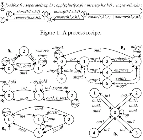
Figure 1 shows an example of a process recipe (based on [8]) that specifies how to assemble a hinge. The first and second p-tasks load a new pallet fixture (f) and sep-arate it into its constituents: the hinge pin (p) and hollow hinge (h). Thenp is glued onto the hinge hto obtain a (non-hollow) hinge (h2), which is then engraved with a serial number. The next two (parallel) tasks involve a 360 degree visual test on h2, after which the recipe ei-ther requests a force test, or discards the hinge, depending on the runtime outcome of the visual test. Similarly, the hinge can be stored or discarded, depending on a further force-test (as these tests are performed at runtime, all al-ternatives must be accounted for).

3

Non-Deterministic Resources

We model manufacturing resources in the facility as la-belled transition systems, and extend [8] by allowing

non-A

B C

E

F D

load(׫,׫,f)  ;;  separate(f,׫,p·∙h)  ;;  applyglue(p,׫,p)  ;;  insert(p·∙h,׫,h2)  ;;  engrave(h,׫,h)  ;; store(h2,׫,h2)

remove(h2,׫,h2)

dotestf(h2,׫,h2)

remove(h2,׫,h2) rotate(׫,h2,׫)  ||  dotestv(h2,׫,h2)

Figure 1: A process recipe.

0 in1,  load 1

out1 remove, store, nop nop R1 0 in3 out3 attgr3,

nop R3

2 applyglue nop, attgr3 2 1 4 3  out1,  out3,   out4  in2  out2 in1  out2,  out3,  out4  out1  in3 in4 R5 0 in4 R4 2 dotestv out4

out4 nop_dotestf

nop

2

load beep

nop

0 1

in2

out2 nop,  hold  

R2 2 in2,  separate out2,  insert nop nop,  hold   4 attgr1 5 attgr2 attgr3 engrave rotate attgr3 6 attgr3 rotate attgr3, nop nop 3 0 1 3 1

Figure 2: An assembly system with non-deterministic resources. The tasks inTinareattgr1, attgr2, attgr3, beep.

deterministic transitions.

Definition 2 (Resource). A resource is a tuple R = ⟨s0, S, T,Ô⇒⟩, whereS is a set of states,s0 ∈ S is the

initial state,T is the set of tasks, andδR⊆S×T×Sis a

transition relation. ∎

We writes_Ô⇒t s′_{to denote a transition from stos}′ _by

task t. For example, resource R1 in Figure 2 can load new pallets. Loading is a non-deterministic transition as it may result in the pallet being misaligned; when this hap-pens, an acoustic signal instructs the operator to realign the pallet. The pallet can then be either stored, removed, or moved to another resource (out1). Transfer of parts be-tween resources is performed by resourceR5, which mod-els a transportation system specifying the “legal routes” between production resources.

A (production) topology represents the synchronous

execution of a set of resources, including where parts are processed and how parts are moved between resources.

Definition 3 (Topology). Let {R1, . . . , Rn} be

re-sources, with eachRi = ⟨s0_i, S_i, T,Ô⇒i⟩. Atopologyis

the set of states;s0= ⟨s0₁, . . . , s0_n⟩is the initial state;Tn

is the set of concurrent tasks; and the transition relation

Ô⇒⊆S×Tn×Sis such thatsÔ⇒t s′iff for alli∈ [1, n]1

either:

• ti/∈Tsynandsi ti

Ô⇒is

′

i, i.e., resourceRican execute

ti;

• ti∈Tsynandsi ti

Ô⇒is′i, and there exists exactly one

j∈ [1, n]such thats_jÔ⇒tj _js′_jwithtj=inhandti= outh _{for someh, denoted t}

j ↢ ti, or the opposite,

denotedtj↣ti. ∎

The second condition checks that, within a transition, eachouttask is matched with anin. A transitions_Ô⇒t s′

is said to beobservableiff at least one task in the vector is observable.

Given a topology⟨s0, S, Tn,Ô⇒⟩, the assignment of

parts to resources during production is represented by a resource vectorr= ⟨c1, . . . ,cn⟩, where eachci∈C∗is a

(possibly empty) sequence of parts that do not appear any-where else inr. We denotecibyr(i)fori∈ [1, n]; the

set of all possible resource vectors asV; and the empty vector asr0 = ⟨, . . . , ⟩. Hence,r(i)denotes the parts

allocated to resourceRiin the current state of the

topol-ogy. We note that each element inr is a sequence and not a set, i.e., order matters when moving parts between resources, or when executing tasks on parts. We address a limitation in [8] by allowing thesimultaneousexecution of tasks on thesameparts, in order to model “joint” tasks. A resourceRicurrently in statesican execute an (atomic)

p-taskt(x,y,z)iff(I) the taskt is available from state s_i inRi, and (II)the input parts are currently assigned

to the resource, and, if external parts are required (i.e., y ≠ ), then there exist one or more other resources to

which those parts are collectively assigned. After execut-ingt, parts inzare allocated to the resource. For example, the taskinsert into(c1, c2, )inserts partc1into partc2, wherec2 is currently assigned to another resource, and does not produce any parts. Given a p-taskt(x,y,z), we

denotexbyin(t),ybyext(t)andzbyout(t).

We now give a formal definition of simultaneous tasks. LetT = t1∥. . .∥tm be a task expression,r a resource

vector, sa topology state, andsÔ⇒t s′ a transition with

t = ⟨t′₁, . . . , t′_n⟩. Let I = {i ∈ [1, n] ∣ t′_i ∈ Tob}be the

1_{s= ⟨s}

1, . . . , sn⟩, s ′= ⟨_s′

1, . . . , s

′

n⟩andt= ⟨t1, . . . , tn⟩.

“observable indices” oft. Then, we say that a resource vectorr′_{is anallocationof}

T totwith respect tor,

de-notedr′

= AL(r,T,t), iff for alli ∈ [1, n] ∖I we have

r′

(i) =r(i), and there exists a bijectionf ∶I ↦ [1, m]

s.t. for alli∈I, we have thatj=f(i)implies

• tj = t′_i, namely the task label in position i in the

vector is equal to the task label of thej-th parallel p-task; and

• r(i) =in(tj),r′(i) = out(tj)andext(tj) ≠ iff

there exists a subset of indicesI′

⊆ [1, n] ∖ {i}such

thatext(tj)is a concatenation of eachin(tk),k∈I′.

Intuitively, an allocation ofT to a topology transition

labelled with vector t returns the new resource vector resulting from the simultaneous execution of each task int, provided that all the p-tasks in T are matched to

an observable task in t. For instance, a vector of tasks t= ⟨hold, nop, engrave⟩can execute a parallel task

ex-pression T = engrave(, c, ) ∥ hold(c, , c), so that ⟨c, , ⟩ = AL(⟨c, , ⟩,T,t). For sequences of the form T1;T2we can compute allocations recursively, and for in-terleaved compositions of the formT1 ∣ T2, we need to find a linearisation such that an allocation exists. Details are omitted for brevity, as they do not differ from [8] apart from the base case above.

For synchronisation tasks, a resource vector r′ _{is a}

transfer of parts fromr viat, denotedr′

= MOV(r,t),

if for eachi∈ [1, n]we have(I)ti↢tjandr′(i) =r(i) ⋅c

with r(j) = c⋅c; or (II) ti ↣ tj and r′(i) = c with

r(j) =c⋅c; or(III)r′(i) =r(i)otherwise. For example,

ifr= ⟨c, , ⟩thenMOV(r,t)witht= ⟨out1, nop, in1⟩is

⟨, , c⟩.

4

Realisability of Recipes

Each transition in a process recipe is labelled with a task expression, but these tasks are not directly executable: ac-tual realisations, in the form of “orchestrations” of the topology, must be found. We now introduce some tech-nical definitions.

Atrace of a topologyPfrom a resource vector r0 is a sequenceτ = σ0Ô⇒t1 σ1Ô⇒⋯t2 such that for eachi ≥0

we haveσi = (s_i,ri), where s_i is a state in the

evolution of the topology,together withthe new resource vector computed at each step. We call a finite trace his-tory, and given a historyτ = σ0Ô⇒⋯t1

tm

Ô⇒σmof length

m, we denoteσmbylast(τ). Unless otherwise specified,

we assumes₀=s0andr0=r0, i.e., we take as initial the

initial state of the topology and the empty resource vector. We now introduce the notion ofplan, which compactly represents the setof histories (there may be more than one, as the topology is non-deterministic) that realise a given task expression. LetHdenote all possible histories

ofP. Then, ahistory-based planis a partial function

π∶ H ↦Tn

which maps a history of P to a vector of tasks. A

trajectory of a plan π on P from σ0 is a trace τ =

σ0Ô⇒t1 σ1Ô⇒⋯t2 of P, of length` ≥ 0, such that ti+1 =

π(τ∣i), where τ∣i denotes the fragment of τ of length

i∈ [0, m−1]. Given a historyτ, we callσ∣τ∣=last(τ)

the outcomeof τ from σ0. A trajectory of πis said to becompletewith respect toπiff it is finite and cannot be extended further, namely, iffπ(τ)is undefined.

4.1

Strong Cyclic Plans

A history-basedterminating planis a plan such that all its trajectories are finite, i.e., it always terminates irrespec-tive of the non-determinism of the topology. However, not all trajectories are finite. For example, in Figure 2, the resourceR3encodes a robotic arm which can perform various operations by attaching different grippers. Since performing theinternal taskattgr3 in state1 may lead to two possible successor states, there is no history-based terminating plan that is guaranteed to realise the recipe, as the observable taskrotatemay never be reached. In reality, while performing a task may occasionally take a resource into an abnormal state, resources are engineered such that after a ‘small’ number of retries and/or some recovery steps, the intended state will be reached.2 _This

‘fairness assumption’ is however not captured explicitly in the resource or the topology.

Note that the appropriate notion of fairness for manu-facturing resources does not correspond tostrong fairness as in [7], where if the action is repeated infinitely often,

2_{Note that there is no restriction in our formalism that the number of}

retries should be small.

then any outcome happens infinitely often. First, while internal tasks such as attgr3 can be non-deterministic, observable tasks such as rotate are assumed to be de-terministic: executing the task is assumed to lead to the intended state—otherwise the author of a process recipe would have to anticipate all possible failures of the (un-known) manufacturing resources used to manufacture the product. In this sense, fairness is only relevant to inter-naltasks, as only internal tasks forming part of the ‘im-plementation’ of an observable task may be retried: e.g., repeatedly executingattgr3will eventually reach a state whererotatecan be executed. Second, repeating an ob-servable task would violate the recipe, and in many cases this would be incorrect and/or unsafe (consider, for in-stance, operations such as casting or moulding). Third, parts/subassemblies often represent considerable invest-ment of materials and process steps, so are usually only discarded as a last resort. As observable tasks may be non-deterministic in practice, a controller may have to implement a ‘recovery’ internal plan fragment to remedy undesired states (e.g., to remove excess material from a moulded part when required) prior to the next observable task in the recipe. Hence, we need to relax strong fairness, and consider a particular kind ofstrong cyclic plan [5] whose associated trajectories can always terminate, and when they do, are guaranteed to achieve the goal.

4.2

Process Plans

We can now concretise our definition of process plan, which represents astrong cyclichistory-based plan. First, we say that a history-based planπisnonblockingif any of its finite trajectoriescanbe extended to a complete trajec-tory (namely, it is a prefix of a complete trajectrajec-tory ofπ). Thus, it is always possible for these plans to terminate. However, they are not necessarilyterminating plans, as they may have infinite trajectories. To be implementable in practice, we need to find afiniterepresentation of such plans.

Definition 4 (Process plan). Given a task expressionT,

a topology states₀and a resource vectorr0, we say that a history-based planπis aprocess planforT from(s₀,r0)

iffπis nonblocking and any complete trajectory ofπfrom

Informally, a trajectoryτ realises an atomic task ex-pressionT iff the task is allocated in (exactly) one step,

which is necessarily an observable transition, while all other steps are arbitrary unobservable transitions (i.e., consisting only of internal tasks and synchronisation tasks). Formally, given a plan π, an initial states₀ and a resource vectorr0, a trajectoryτ =σ0

t1

Ô⇒⋯

tm

Ô⇒σmof

πfromσ0, withσi= (s_i,ri)for eachi∈ [1, m]realises

an atomic task expressionT iff:

• there exists an`∈ [1, m]such thatr`= MOV(r,t`)

withr=AL(r`−1,T,t`);

• for any otherj ≠ `,j ∈ [1, m], we have that tj is

unobservable andr`=MOV(r`−1,t`).

We extend this notion to sequences, and say that a tra-jectoryτ realises a task expression of the formT1;T2iff

τ has the formτ = τ1⋅τ2 andτ1 (resp. τ2) realisesT1 (resp.T2), whereτ1⋅τ2denotes the concatenation of two finite trajectories sharing the last and first state, respec-tively (which is equal toτ1whenτ2is the empty trajec-tory). The extension to interleaved compositions is anal-ogous, by considering all possible linearisations. Without loss of generality, we assume that an observable transition is always the last one in the trajectory, as this strictly re-lates plans to the task expressions that they realise by dis-allowing subsequent arbitrary transitions (which, instead, should be executed to realise thenexttask expression in the recipe).

As process plans are not necessarily terminating, they may have infinite trajectories. We therefore introduce fi-nite representations of such plans. First, given a historyτ, itscontractions, denotedacycl(τ), is the set of histories

obtained fromτby removing all cycles. The contractions correspond to the fixpoint of an operatorλon{τ}defined

asτ1⋅τ2∈λ({τ,⋯})iffτ =τ1⋅τ′⋅τ2, such that the first and last state ofτ′_{are the same, i.e.,last}

(τ1) =last(τ′).

It is trivial to see that a contraction always exists. Abasic planis a partial function

πb∶ Ha↦Tn

that is defined only for acyclic histories Ha ⊆ H of P

(which are finite), and thus only generates finite and com-plete trajectories. We say thatπbis abasic plan forT iff

every acyclic trajectory ofπbthat is complete realisesT,

and at least one such trajectory exists. These plans can be represented and implemented finitely; however, they are not process plans: they do not need to realise any task, and indeed in a non-deterministic topology they may not do so. Given a basic planπb, we can reconstruct a generic

history-based planπ{πb}as follows:

π{πb}(τ) ∶=πb(τ) iff it is defined;

π{πb}(τ) ∶=π{πb}(τ ′

) otherwise,

whereτ′_{is a trajectory ofπ}

b andτ′ ∈ acycl(τ).

Infor-mally,πbis applied toτby disregarding any cycle.

Theorem 1. Ifπbis a basic plan forT andπ{πb}is

non-blocking, thenπ{πb}is a process plan forT.

Proof Sketch.It is easy to see thatπbis defined for every

contraction of one of its trajectories that still does not re-aliseT. This holds trivially for acyclic trajectories, since

they must realise the task expression by definition. For cyclic trajectories, assume that for a contractionτ′_,π

b(τ′)

is undefined. Then τ′

is not a trajectory of πb (which

is instead required) otherwise, being complete, it would contradict the fact that every complete acyclic trajectory realisesT. Hence any cyclic trajectory ofπ{πb}can

al-ways be extended to one that is finite and complete. Thus π{πb}is nonblocking, which together with the hypothesis

proves the claim. ◻

Basic plans are memory bounded, and as soon as they induce a cyclic trajectory, they immediately “reset” to a contraction. However, not every process plan can be re-constructed from a given basic πb (e.g., a process plan

that prescribes a different action for the same cyclic be-haviour of the system when the number of cycles is a prime number). Nevertheless, the result above is crucial for computing the “correct” set of basic plans πb for a

task expression T (i.e., those where π{πb} is

nonblock-ing). It can be shown that fromthe setof allbasic pro-cess plansΠ¯ = {π1, . . . , πq}for a task expressionT such

thatπ{πi}is nonblocking, we can reconstructanyprocess

planπforT. The proof of this claim is involved and we

omit it due to lack of space, as it is not needed to prove the correctness of our approach. Rather it supports (in addition to Theorem 1) the intuition that basic plans rep-resent the minimum information required to reconstruct process plans. Intuitively, a process plan forT can be

that prescribes, at each step of the current trajectory τ, which basic planπf(τ)to use.

4.3

Process-Plan Simulation Relation

In this section, we capture the ability to realise transitions in the recipe as apropertyrelating states of the recipe with states of the topology and resource vectors.

Definition 5. LetP= ⟨s0, S, T,Ô⇒⟩ be a topology and

R = ⟨s0, S, L, δR⟩a recipe. Aprocess-simulation

rela-tion is a relationPSIM ⊆ S×S×V,3 such that a tuple ⟨s, s,r⟩ ∈PSIMimplies that for anyT, ifs_ÐT_→s′for some s′_{, then there exists a process planπ such that for each}

complete trajectoryτ ofπfrom(s,r), we have that(I)τ

realisesT (as defined above); and(II)⟨s′, s′,r′⟩ ∈ PSIM, where(s′,r′) =last(τ).

Thus, a statesof a recipeRis said to be

process-simu-latedby a statesof a topologyPwith respect to a resource vectorrif there exists a process-simulation relationPSIM

such that⟨s, s,r⟩ ∈PSIM. Moreover,R = ⟨s0, S, L, δR⟩is

process-simulated byP= ⟨s0, S, T,Ô⇒⟩ifs0is

process-simulated bys0with respect tor0.

The definition states that no matter how the recipe evolves froms(according to transition choices made by runtime tests), there exists a process plan whose complete trajectories realise the requested task expression. Cru-cially, the process recipe cannot control which particular trajectory of the process plan is followed, as the topology is non-deterministic.

Definition 6 (Realisability of a recipe). Given a states₀ and a resource vectorr0, a recipeR = (s0, S, L, δR)is

realisablefrom(s₀,r0)iff there exists a functionω∶S× V ×δR↦Πsuch that:

• for each transition s0T

Ð→s

′ _in

R, the plan ω(s₀,r0, s0ÐT→s

′

) = π is defined and it is a

process plan forT from(s₀,r0);

• ifω(s,r, s_ÐT_→s′) =πis defined, then

– πis a process plan forT from(s,r); and

3_{Recall thatV is the set of all resource vectors.}

– for each outcome(s′,r′)of a complete

trajec-toryτofπfrom(s,r), and for eachs′ T

′

Ð→s

′′_in

R, we have thatω(s′,r′, s′ T

′

Ð→s

′′

)is defined.∎

Recall that ifπis a process plan for T from σ, then

any complete trajectory ofπfromσrealisesT. Finally, a

recipeRisrealisablein atopologyP= ⟨s0, S, T,Ô⇒⟩if Ris realisable from(s0,r0). The above definition only

requires theexistenceof a functionωwhich returnsa pos-sible“correct” plan at each step. The notion of realisabil-ity in a topology is closely related to the notion of plan-based simulation in [6] and T-realisation in [7].

How-ever, unlike that setting, we do not consider a planning domain due to the high modularity of our setting, as well as the presence of various low-level details (such as re-source vectors and simultaneous tasks).

Theorem 2. A process recipeRis realisable in a

topol-ogyPiffPprocess-simulatesR.

Proof Sketch. Given (s,r), assume that a function

ω as above is defined for each sT

Ð→s

′ _in

R, namely, ω(s,r, s_ÐT_→s′) = π, but P does not process-simulateR.

By Def. 5 this implies that there is no process plan, in-cludingπ, such that each of its complete trajectories τ realiseT, or the⟨s′, s′,r′⟩ /∈PSIMwith(s′,r′) =last(τ).

These two cases violate the first and second item of Def. 6, respectively; hence,ω does not exist. If instead

⟨s0, s0,r0⟩ ∈PSIM, then, by definition, there exists a plan πas in Def. 5 for eachs0T

Ð→s

′_in

R; hence, we can build

the functionωso thatω(s0,r0, s0ÐT→s′) =π. The same

ar-gument can be applied by induction on⟨s′, s′,r′⟩, where (s′,r′)is the outcome of any complete trajectory ofπ, as ⟨s′, s′,r′⟩ ∈PSIMby hypothesis. ◻

4.4

Process Plan Controllers

Definition 7. Given a topologyPand process recipeR, a

process plan controllerforR = ⟨s0, S, Lang(T ), δR⟩in

Pis a tupleC = ⟨PSIM, δR,Π, δ⟩with:

• PSIM ≠ ∅ is a process plan-simulation relation,

whose elements correspond to the set of states in the controller;

• δRis the recipe transition relation;

• Πis a set of process plans;

• δ∶PSIM×δR×Π×PSIMis a transition relation,

defin-ing transitions from one state to another, by execut-ing a process planπthat realises a task expression

T. A transition⟨s′, s′,r′⟩ ∈δ(⟨s, s,r⟩, tr, π)exists

fortr=s_ÐT_→s′, also denoted⟨s, s,r⟩_Ðtr,π_Ð→⟨s′, s′,r′⟩,

iffsT

Ð→s

′_{is inδ} Rand:

– πis a process plan forT, i.e., it is nonblocking

and all complete trajectories ofπrealiseT;

– a complete trajectoryτofπexists from(s,r)

with(s′,r′) = last(τ), and for any complete

trajectoryτ′ _{ofπ from}

(s,r)with(s′′,r′′) = last(τ′), we have⟨s, s,r⟩_Ðtr,π_Ð→⟨s′′, s′,r′′⟩. ∎

As a direct consequence of Theorem 2 and the defini-tion of process plan controller, we get the following result.

Theorem 3. A recipeRis realisable in a topologyPiff

there exists a process plan controller forRinP.

Proof Sketch. It follows by construction of the process plan controller C. It is possible to compute the

func-tionω in Definition 6 as follows: ω(s,r, s_ÐT_→s′) = πiff ⟨s, s,r⟩Ðtr,πÐ→⟨s′, s′,r′⟩, considering tr = sÐT→s′. Indeed

by Theorem 2 if ⟨s, s,r⟩ ∈ PSIM then ω(s,r, s_ÐT_→s′)is

defined for every recipe transitionsT

Ð→s

′

. ◻

5

Computing Basic Plans

In this section, we provide an algorithm that computes a process-plan simulation relation given a process recipeR

and a topologyP, and in doing so also computes a process plan controller forRandP. We extend the algorithms in

[8] to handle non-deterministic topologies and to compute

Algorithm 1FINDSIM(R,P, s,r, s)

Input: a process recipeR = (s0, S, L, δR), a topologyP, the

topology states, resource vectorrand recipe states. 1: δ, δ′

,PSIM,PSIM′:=∅

2: foreach recipe transitiontr= (s,T, s′) ∈ δRdo

3: (PSIM′, δ′

):= EVAL(R,P,T, tr,(s,r), π_b0,(s,r),∅)

4: ifPSIM′

= ∅then return(∅,∅)

5: PSIM:=PSIM∪PSIM′;δ:=δ∪δ′

6: return (PSIM∪ {(s, s,r)}, δ)

asetof basic plans, having the property as in Theorem 1, for each transition of the process recipe. By the theorem, these can be used to reconstruct history-based plans.

Given a process recipe R, a topology P, a state sof

P, a resource vector rand a state sof R, Algorithm 1

determines, for each transitiontr=s_ÐT_→s′, whether there

exists a basic plan forT from(s,r), and in turn, whether

the same holds for each transition froms′

(as required by Definition 6). To this end,tris passed as a parameter to Algorithm 2 to continue checking froms′_{. We useπ}0

b to

denote the empty plan.

Algorithm 2 uses two auxiliary functions: given a task expressionT = T1;T2;. . .;Tn with n > 0, the first

el-ement ofT is defined as FST(T ) = T1 and the rest of its elements as RST(T ) = T2;. . .;Tn if n > 1, and as RST(T ) =ifn=1. Intuitively, Algorithm 2 performs a

depth-first search of the topology to check whether there exists a basic plan for the task expressionTcur (initially

T) fromσ↓. In particular, the outer loop (lines 9 to 33)

considers each unique label tin the outgoing topology transitions froms_↓; lines 11 to 19 apply iftis observable and the first task inTcur can be allocated to it, and lines

20 to 32 apply iftis unobservable.

For each observable transition associated with a par-ticular label t, lines 12 to 18 prescribe the following. First, the “successor” coupleσ= (s,r)is created to

rep-resent the allocation ofTcur tot, and the movement of

parts via synchronisations. Second, line 14 updates the planπbwith the vectortlabelling the topology transition

(s_↓,t, s); this plan is then passed as a parameter in the

recursive call to EVAL. Finally, if the rest of the tasks in

Tcurcannot be realised fromσ, all non-deterministic

tran-sitions labelled withtare disregarded. Otherwise, new tu-ples inPSIMsand the corresponding controller transition

Algorithm 2EVAL(R,P,Tcur, tr, τ, πb, σ0,Σ)

Input: a process recipeR, a topologyP = (s0, S, Tn,Ô⇒),

the current task expressionTcurand recipe transitiontr= (s,T, snxt), the current trajectoryτ and basic planπb, the

initial coupleσ0= (s₀,r0)and the visited couplesΣ.

1: σ↓:=(s↓,r↓):=last(τ)

2: (PSIM, δ):=(∅,∅)

3: ifTcur=then

4: x:=(s₀, s,r0)Ðtr,πÐÐ→(b s↓, snxt,r↓)

5: (PSIM, δ):= FINDSIM(R,P, s↓,r↓, snxt)

6: return (PSIM, δ∪ {x})

7: ifσ↓∈Σthen return({σ↓},∅)

8: σfst:=

9: foreachtsuch that(s_↓,t, s)exists inÔ⇒do

10: (PSIMt, δt):=(∅,∅)

11: iftis observable andr′

=AL(r↓,FST(Tcur),t) then

12: foreach(s_↓,t, s) ∈ Ô⇒ do

13: σ:=(s,MOV(r′

,t))

14: πb(τ):=t

15: (PSIMs, δs):=

EVAL(R,P,RST(Tcur), tr, τ_Ô⇒t σ, πb, σ0,∅)

16: ifPSIMs= ∅then(PSIMt, δt):=(∅,∅);break

17: else(PSIMt, δt):=(PSIMt∪PSIMs, δt∪δs)

18: end for

19: (PSIM, δ):=(PSIM∪PSIMt, δ∪δt)

20: else iftis unobservablethen

21: foreach(s_↓,t, s) ∈ Ô⇒do

22: σ:=(s,MOV(r↓,t))

23: πb(τ):=t

24: Σ′

:=Σ∪ {σ↓}

25: (PSIMs, δs):=

EVAL(R,P,Tcur, tr, τÔ⇒t σ, πb, σ0,Σ′)

26: ifPSIMs= ∅then

27: (PSIMt, δt):=(∅,∅);σfst:=;break

28: else ifPSIMs= {σ′}andδs= ∅then

29: σfst:=EARLIER(σfst, σ

′

, τ)

30: else(PSIMt, δt):=(PSIMt∪PSIMs, δt∪δs)

31: end for

32: (PSIM, δ):=(PSIM∪PSIMt, δ∪δt)

33: end for

34: ifPSIM≠ ∅then return(PSIM, δ)

35: else ifσfst/∈ {, s_↓}then return({σfst},∅)

36: else return(∅,∅)

is unobservable, the steps are similar to those described above, except for lines 28 and 29. Line 28 applies to the case in which τ_Ô⇒t σ constitutes a cycle “back” in the

current trajectoryτ(i.e., line 7 was executed in the recur-sive call at line 25): if this is the case, then we compare σ′_{with the stateσ}

fst (initially the empty string) which is

the “earliest” state that is possible to reach, through cy-cles, from the current topology states↓. The intuition is

as follows: we need to make sure that thereexiststhe pos-sibility, fromσ↓, to cycle back to a stateσfst from which

it is still possible to find a complete trajectory whose ex-ecution allocates the task expressionTcur. If this is the

case, then the cycle in the current trajectory of planπbis

“admissible”: it (still) guarantees the nonblocking condi-tion of the planπ{πb}. Formally, we define the function

EARLIER(σ1, σ2, τ) =σ1ifσ1occurs beforeσ2inτ(or

σ2=), andEARLIER(σ1, σ2, τ) =σ2ifσ2occurs before

σ1 inτ (orσ1 = ). Then(PSIM, δ)is returned in line

34, consisting of the simulation relations and correspond-ing controller’s transitions. Otherwise, we must rely on there being a state that appears inτ before s_↓, and pos-sibly as early asσfst, from where a complete trajectory

can be found and the task allocated. Thus, we “propagate back”σfst until we can exit the current cycle, or until the

recursive step is reached withσ↓ = σfst, from where an

exit must then exist if a non-empty simulation relation is to be returned. Line 7 checks whether the algorithm has reached a couple σ↓ visited earlier, and if so returns it,

guaranteeing that the plan is bounded.

A variant of this algorithm for deterministic topolo-gies has been implemented as part of an agent based con-trol architecture for manufacturing, designed to address rapidly changing product and process requirements [9]. Within this architecture, a process plan controller is used to select basic plans for task expressions that appear in the recipe. Such plans are represented in the Behaviour to Markup Manufacturing Language (B2MML) ISA-95 standard, which is a format that is interpretable by real-world manufacturing execution systems. The implemen-tation also takes into account additional details such as parameters and materials, which have been omitted in this paper.

6

Related Work

produc-tion topologies as planning goals and planning domains. In our setting, there are several features that make such an encoding difficult, including conditional goals (in the recipe), interleaved and parallel tasks.

The notion of process plan controller is closely re-lated to other approaches. For exampleagent planning programs [7, 6] are finite-state programs where transi-tions prescribe propositional achievement and mainte-nance goals that must be realised on a planning domain by implementing each transition via a conditional plan. The solution approach is based on restricted forms of LTL syn-thesis, and is able to cope with non-deterministic proposi-tionalplanning domains with explicit fairness constraints, thus producing strong cyclic plans. However, as explained in Section 4.1, the manufacturing setting has a number of features which preclude a straightforward application of this approach, and standard notions of strong cyclic plan-ning cannot be applied.

Our notion of a terminating plan is also similar to history-based terminating plans in [6], and related to the notion of (memoryless) strong acyclic plans [5]. As we explain in Section 4.1, our approach differs from [6] in that the trajectories we consider are not finite. Simi-larly, the state-action table representation used for strong acyclic plans in [5] is insufficiently flexible for process plans, as it is memoryless, whereas in our setting we must choose actions based on the current history (evolution of the topology) rather than simply the current state of the topology.

Over the last decade there has been a growing body of work on automation to achieve flexibility, resilience, and monitoring in manufacturing. For example,Flexible Manufacturing Systems[3, 17, 10] increase the variety of parts and products that can be produced, while Reconfig-urable Manufacturing Systems[2, 12, 14, 18] allow more rapid response to market changes for a certain product family. In [11] an approach is presented to the synthe-sis of controllers capable of producing multiple instances of the same product simultaneously. However, as none of this work has addressed the manufacture of products in the context of manufacturing as a service, nor considered fairness assumptions or differentiated observable and un-observable tasks, they are restricted to acyclic plans when resources are non-deterministic.

7

Conclusions and Future Work

We extended previous approaches to the realisability and control problems for process recipes in manufacturing systems consisting of non-deterministic resources, and where operations can be performed in parallel on the same part. We formally defined the notions of process plans and process plan controllers for these systems, where loops in plans must be allowed due to intrinsic fairness assump-tions. In this paper we assume that a manufacturing fa-cility is always initially in the initial state of the topology with an empty resource vector. In future work, we plan to relax this assumption and generalise our approach to consider an arbitrary initial state, where parts are already assigned to resources, and the topology is currently being orchestrated to realise another process recipe.

References

[1] A Landscape for the Future of High Value Manu-facturing in the UK. Technical report, Technology Strategy Board, 2012.

[2] Zhuming M. Bi, Sherman Y.T. Lang, Weiming Shen, and Lihui Wang. Reconfigurable manufacturing sys-tems: the state of the art. International Journal of Production Research, 46(4):967–992, 2008.

[3] Jim Browne, Didier Dubois, Keith Rathmill, Suresh P. Sethi, and Kathryn E. Stecke. Classifi-cation of flexible manufacturing systems. The FMS magazine, 2(2):114–117, 1984.

[4] J. C. Chaplin, O. J. Bakker, L. de Silva, D. Sander-son, E. Kelly, B. Logan, and S. M. Ratchev. Evolv-able assembly systems: A distributed architecture for intelligent manufacturing. In A. Dolgui, J. Sasi-adek, and M. Zaremba, editors, 15th IFAC Sym-posium on Information Control Problems in

Man-ufacturing (INCOM 2015), volume 48 of

IFAC-PapersOnLine, pages 2065–2070, Ottawa, Canada,

May 2015. Elsevier.

[6] Giuseppe De Giacomo, Alfonso Emilio Gerevini, Fabio Patrizi, Alessandro Saetti, and Sebastian Sardi˜na. Agent planning programs. Artificial In-telligence, 231:64–106, 2016.

[7] Giuseppe De Giacomo, Fabio Patrizi, and Sebas-tian Sardi˜na. Generalized planning with loops un-der strong fairness constraints. InInternational Con-ference on Principles of Knowledge Representation and Reasoning, pages 351–361, 2010.

[8] Lavindra de Silva, Paolo Felli, Jack C. Chap-lin, Brian Logan, David Sanderson, and Svetan Ratchev. Realisability of production recipes. In G. A. Kaminka, M. Fox, P. Bouquet, Hullermeijer E., Dignum F., Dignum V., and van Harmalen F., ed-itors,Proceedings of the 22nd European Conference on Artificial Intelligence (ECAI), pages 1449–1457. IOS Press, 2016.

[9] Lavindra de Silva, Paolo Felli, Jack C. Chap-lin, Brian Logan, David Sanderson, and Svetan Ratchev. Synthesising industry-standard manufac-turing process controllers. In Proceedings of the International Conference on Autonomous Agents

and Multiagent Systems (AAMAS), pages 1811–

1813, 2017. Accompanying video available at: https://youtu.be/SEveuikI3p8.

[10] Hoda A. ElMaraghy. Flexible and reconfig-urable manufacturing systems paradigms. Interna-tional Journal of Flexible Manufacturing Systems, 17(4):261–276, 2005.

[11] Paolo Felli, Brian Logan, and Sebastian Sardina. Parallel behavior composition for manufacturing. In Subbarao Kambhampati, editor, Proceedings of the 25th International Joint Conference on Artificial In-telligence (IJCAI 2016), pages 271–278, 2016.

[12] Yoram Koren, Uwe Heisel, Francesco Jovane, Toshimichi Moriwaki, G. Pritschow, G. Ulsoy, and H. Van Brussel. Reconfigurable manufacturing systems. CIRP Annals-Manufacturing Technology, 48(2):527–540, 1999.

[13] Yuqian Lu, Xun Xu, and Jenny Xu. Development of a hybrid manufacturing cloud. Journal of Manufac-turing Systems, 33(4):551–566, 2014.

[14] Mostafa G. Mehrabi, A. Galip Ulsoy, and Yoram Koren. Reconfigurable manufacturing systems: key to future manufacturing.Journal of Intelligent Man-ufacturing, 11(4):403–419, 2000.

[15] Dana Nau, Malik Ghallab, and Paolo Traverso.

Automated Planning: Theory & Practice.

Mor-gan Kaufmann Publishers Inc., San Francisco, CA, USA, 2004.

[16] Chris Rhodes.Manufacturing: Statistics and Policy. Briefing Paper. House of Commons Library, 2015.

[17] Andrea Krasa Sethi and Suresh Pal Sethi. Flexibility in manufacturing: a survey. International Journal of Flexible Manufacturing Systems, 2(4):289–328, 1990.