A Thesis Submitted for the Degree of PhD at the University of Warwick
http://go.warwick.ac.uk/wrap/36337
This thesis is made available online and is protected by original copyright. Please scroll down to view the document itself.
WARWICK
BUSINESS.SCHOOLUsing Non-Linear/Chaotic Dynamics for Interest Rate
Determination
Julian H. Tice
WAkWIC1K
Thesis submitted for the Degree of PhD Industrial and Business Studies
September 1998
ACKNOWLEDGEMENTS DECLARATION
SUMMARY
1. INTRODUCTION 1
1.1 SHOULD THE SHORT TERM INTEREST RATE DRIFT BE CONSIDERED NON-LINEAR9 4
1.2 CONTRIBUTION AND OUTLINE 7
2. DYNAMIC MEAN INTEREST RATE MODELS AND THE IS-LM FRAMEWORK... 10
2.1 INTRODUCTION 11
2.2 A DYNAMIC MEAN FRAMEWORK 12
2.3 THE IS-LM FRAMEWORK 14
2.4 ASSESSING THE DYNAMICS OF THE TWO FACTOR MODEL 18
2.5 CONCLUSIONS 26
3. A THREE FACTOR MODEL 27
3.1 INTRODUCTION 28
3.2 EXTENDING THE TWO FACTOR MODEL 29
3.3 ASSESSING THE DYNAMICS OF THE MODEL; THE RELATION TO LORENZ 32
3.4 ESTIMATION AND PRICING ISSUES 41
3.4.1 Observability, ensembles and noise 50
3.4.2 The exercise of control 56
3.5 CONCLUSIONS 58
4. AN ESTIMATION PROCEDURE 59
4.1 INTRODUCTION 60
4.2 ESTIMATION PROCEDURE FOR t, MO, Xr, Gr 61
4.3 THE REMAINING PARAMETERS: LINEAR REGRESSION APPROACH 62
4.3.1 Estimation procedure for a 63
4.3.2 Estimation procedure for p 63
4.3.3 Estimation procedure for ot and f3 concurrently 64
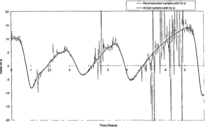
4.3.4 Recovering the path for p 66
4.3.5 Estimation procedure for y, 8, and 4) 67
4.4 APPLICATION TO SIMULATED DATA 67
4.4.1 Estimating a and 3 69
4.4.2 Recovering the path for p 72
4.4.3 Estimating y, 8, and0 75
4.5 SOME ALTERNATIVE APPROACHES 80
4.6 CONCLUSION 81
APPENDIX 4-1: BOND PRICING EQUATION APPROXIMATION 82 APPENDIX 4-2: FORMULA FOR LAGRANGIAN POLYNOMIAL 83
5. A BETTER APPROACH: THE KALMAN FILTER 84
5.1 INTRODUCTION 85
5.2 THE USE OF KALMAN FILTERING: A REVIEW 86
5.3 IMPLEMENTATION ISSUES 87
5.3.1 The traditional Kalman Filter 88
5.3.2 Square Root Methods and the Molf-Kailath Filter 90
5.4 THE BABBS AND NOWMAN (1997) MODEL AND USE OF APPROXIMATED TERM STRUCTURE 107
5.4.1 Introduction 107
5.4.2 The Babbs and Nowman (1997) model 108
5.4.3 Investigating the case where the exact solution to the bond pricing equation is
unknown 113
5.4.4 Empirical investigation into the use of approximations and derivatives of the term
structure 122
5.4.5 Further Kalman Filter estimates for the Babbs and Nowman model 128
5.5 ESTIMATION OF THE DYNAMIC MEAN MODELS WITH THE KALMAN FILTER 138
5.5.1 Estimation of the two factor model 140
5.5.2 Estimation of the three factor model. 143
5.6 CONCLUSION 152
APPENDIX 5-1: ALGORITHM FOR HOUSEHOLDER REDUCTION OF A MATRIX TO UPPER TRIANGULAR
FORM 153
APPENDIX 5-2: ALGORITHM FOR COMPUTING THE DERIVATIVE OF A CHOLESKY FACTOR OF A
SYMMETRIC MATRIX 153
6. CONCLUSION 156
6.1 FURTHER RESEARCH 158
FIGURE 2-1: THE EVOLUTION OF r AND x FOR SYSTEM (2.3-5) Cr = 0.025, C5 = ... ... 2222
FIGURE 2-2: THE EVOLUTION OF r AND x FOR SYSTEM (2.3-5) C ... r =0, Gx = 0 FIGURE 2-3: THE SOLUTION PATH IN r AND x SPACE Cr=0.025, (Tx- 0 ... 24...
FIGURE 2-4: THE SOLUTION PATH IN r AND x SPACE 6r =0, (Tx= 0 ... ... 24
FIGURE 2-5: THE DYNAMICS OF THE SOLUTION PATH IN THE IS-LM FRAME Cr ='0.025, (Tx 0 25 FIGURE 2-6: THE DYNAMICS OF THE SOLUTION PATH IN THE IS-LM FRAME Cfr ° "... 25
... FIGURE 3-1: THE EVOLUTION OF r ... 33
FIGURE 3-2: THE ATTRACTOR IN (r,p) SPACE ... ... 35
FIGURE3-3: UK INTEREST RATE 1954-1994 ... ... ... 36
FIGURE3-4: AN ILLUSTRATIVE EVOLUTION OF r ... ... 36
FIGURE3-5: SHORT RATE PATH INCLUDING NOISE; 6 = 0.02 ... 39
FIGURE 3-6: SHORT RATE PATH WITHOUT NOISE; CY = 0 . ... FIGURE 3-7: THE ATTRACTOR IN (r,p) SPACE TE WITH NOISE;
a
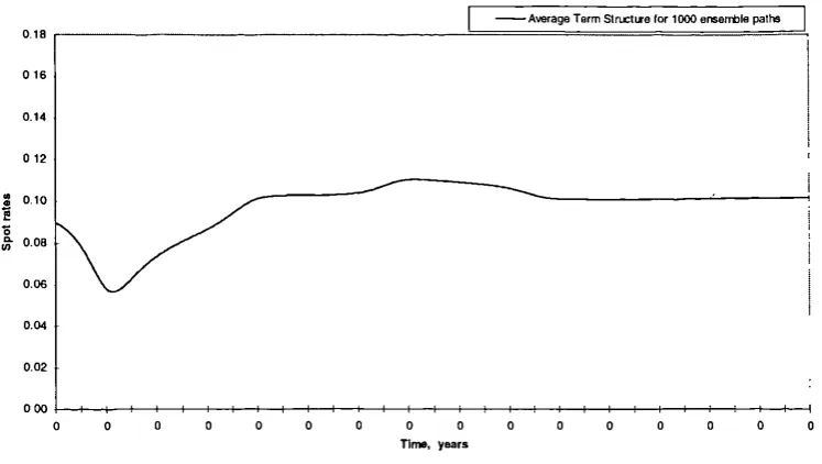
= 0.02 ... 444002FIGURE 3-8: THE TERM STRUCTURE OF INTEREST RATES: A MONTE CARLO ESTIMATE ... FIGURE3-9: PERSPECTIVE OF z t FOR n = 3 49
FIGURE3-10: SECOND PERSPECTIVE OF Zr FOR n = 3 49
FIGURE 3-11: DETERMINISTIC TERM STRUCTURES FOR PATHS A AND B 51
FIGURE3-12: EVOLUTION OF THE TERM STRUCTURE 51
FIGURE3-13: DETERMINISTIC SAMPLE P ATH FOR F IGURE 3-12 52
FIGURE 3-14: THE DISTRIBUTION OF TERMINAL VALUES FOR r: AN ENSEMBLE ESTIMATE 53
FIGURE 3-15: TERMINAL VALUES FOR r: x0 IN THE RANGE [0.02,0.18] 53
FIGURE 3-16: THE DISTRIBUTION OF TERMINAL VALUES FOR r: A STOCHASTIC ESTIMATE 54 FIGURE 3-17: THE TERM STRUCTURE OF INTEREST RATES: AN ENSEMBLE ESTIMATE 55 FIGURE 3-18: CONTROL OF p 57 FIGURE 4-1: RECONSTRUCTED SAMPLE PATH FOR p, 73 FIGURE 4-2: SUBSEQUENCE OF TIME INDEXES OF RECOVERED SAMPLE PATH FOR pr CHOSEN UNDER CRITERION Ir, - ]..1.1> 0.01 75 FIGURE 5-1: SIMULATED B&N PROCESS. THEORETICAL INSTANTANEOUS SHORT RATE SAMPLE PATH (TAU = 0 YRS) 116 FIGURE 5-2: SIMULATED B&N PROCESS. THEORETICAL 3, 6 MONTH AND 1 YR RATE IMPLIED BY SAMPLE PATH IN FIGURE 5-1 116
FIGURE 5-3: THEORETICAL SLOPE OF TERM STRUCTURE AT TAU = 0.25, 0.5, 1 YRS IMPLIED BY SAMPLE PATH IN FIGURE 5-1 118
FIGURE 5-4: THEORETICAL CURVATURE OF TERM STRUCTURE AT TAU = 0.25, 0.5, 1 YRS IMPLIED BY SAMPLE PATH IN FIGURE 5-1 118 FIGURE 5-5: COMPARISON OF OBSERVED AND ESTIMATED 3 MONTH INTEREST RATE 123 FIGURE 5-6: COMPARISON OF LAGRANGIAN EMPIRICAL SLOPE AND THEORETICAL SLOPE FOR THE
TERM STRUCTURE AT TAU = 3 MONTHS 124
FIGURE 5-7: COMPARISON OF LAGRANGIAN EMPIRICAL SLOPE AND THEORETICAL SLOPE AT TAU =
7YRS 125
FIGURE 5-8: LAGRANGIAN EMPIRICAL SLOPE OF TERM STRUCTURE FOR MATURITIES 3 MONTH
THROUGH 10 YEAR 126
FIGURE 5-9: COMPARISON OF LAGRANGIAN EMPIRICAL CURVATURE AND THEORETICAL IMPLIED
CURVATURE AT TAU =6 MONTHS 126
FIGURE 5-10: LAGRANGIAN EMPIRICAL CURVATURE OF TERM STRUCTURE FOR MATURITIES 3
MONTH THROUGH 10 YEAR 127
FIGURE 5-11: COMPARISON OF IMPLIED THEORETICAL SLOPE FROM ONE FACTOR ESTIMATES WITH
LAGRANGIAN EMPIRICAL VALUES 134
FIGURE 5-12: COMPARISON OF IMPLIED THEORETICAL CURVATURE FROM ONE FACTOR ESTIMATES
FIGURE 5-13: COMPARISON OF IMPLIED THEORETICAL SLOPE FROM TWO FACTOR ESTIMATES WITH
LAGRANGIAN EMPIRICAL VALUES 137
FIGURE 5-14: SAMPLE PATH FOR PARAMETER VALUES IN TABLE 5-12 145 FIGURE 5-15: SPECTRAL RADIUS OF STM ASSOCIATED WITH SAMPLE PATH IN FIGURE 5-14 146 FIGURE 5-16: ERROR FOR OFF DIAGONAL ELEMENTS OF ERROR COVARIANCE MATRIX FOR CKF 146 FIGURE 5-17: ERROR ON ESTIMATE FOR p (CKF) 147 FIGURE 5-18: ERROR ON ESTIMATE FOR p (SRCF) 148
FIGURE 5-19: ACTUAL PATH FOR p 148
List of Tables
TABLE 2-1: COMPARISON OF TERM STRUCTURE MODELS 12 TABLE 2-2: PARAMETER VALUES USED FOR FIGURE 2-1 TO FIGURE 2-6 21 TABLE 3-1: SENSITIVITY OF BOND OPTION PRICES TO PARAMETER VALUES 43 TABLE 3-2: SENSITIVITY OF BOND PRICES TO PARAMETER VALUES 44 TABLE 3-3: PCA RESULTS FOR UK MONEY MARKET DATA 48 TABLE 4-1: PARAMETER VALUES USED FOR SIMULATED ANALYSIS 68 TABLE 4-2: MONTE CARLO ESTIMATES OF [I AND 6 68 TABLE 4-3: MONTE CARLO SIMULATION ESTIMATES FOR a AND 13 71 TABLE 4-4: MONTE CARLO ESTIMATES FOR y, 8, 0 USING EXACT p, 76
TABLE 4-5: MONTE CARLO ESTIMATES FOR 7, 5, 4) USING EXACTA AND SECOND ORDER TERMS 77 TABLE 4-6: MONTE CARLO ESTIMATES FOR y, 8, (1) USING RECOVERED pi t AND SELECTED TIME
INDEXES 78
TABLES-I: PARAMETERS USED TO SIMULATE ONE FACTOR B&N PROCESS 115 TABLE 5-2: MONTE-CARLO ESTIMATES FOR THE MSE BETWEEN THE THEORETICAL AND
APPROXIMATED TERM STRUCTURE 117
TABLE 5-3: MONTE CARLO ESTIMATES FOR THE MSE BETWEEN THE THEORETICAL AND
APPROXIMATED SLOPE AND CURVATURE 119
TABLE 5-4: MONTE-CARLO ESTIMATES OF THE MSE FOR THE LAGRANGIAN ESTIMATES OF SLOPE
AND CURVATURE AGAINST THEORETICAL VALUES 121
TABLE 5-5: MONTE-CARLO ESTIMATES FOR THE EXPECTED STANDARD DEVIATIONS OF THE
MEASUREMENT ERRORS ON THE SLOPE AND CURVATURE 122 TABLE 5-6: COMPARISON OF ESTIMATES FOR ONE AND TWO FACTOR MODELS AS ESTIMATED BY
BABBS AND NOWMAN (1997) AND TICE (1998) 130
TABLE 5-7: MODELS ESTIMATED FOR ONE AND TWO FACTOR GENERALISED VASICEK PROCESS 131 TABLE 5-8: COMPARISON OF ESTIMATES FOR ONE FACTOR GENERALISED VASICEK PROCESS USING
THEORETICAL AND APPROXIMATED TERM STRUCTURE 132
TABLE 5-9: COMPARISON OF ESTIMATES FOR TWO FACTOR GENERALISED VASICEK PROCESS USING
THEORETICAL AND APPROXIMATED TERM STRUCTURE 136
TABLE 5-10: MODELS ESTIMATED FOR TWO AND THREE FACTOR DYNAMIC MEAN PROCESSES 139 TABLE 5-11: PARAMETER ESTIMATES FOR DYNAMIC MEAN TWO FACTOR MODEL 142 TABLE 5-12: PARAMETER VALUES USED FOR SIMULATED PATH IN FIGURE 5-14 144 TABLE 5-13: PARAMETER ESTIMATES FOR DYNAMIC MEAN THREE FACTOR MODEL 149
List of Algorithms
ALGORITHM 5-1: UNCOVERING THE DERIVATIVE OF A UPPER TRIANGULAR CHOLESKY FACTOR 103 ALGORITHM 5-2: UNCOVERING THE DERIVATIVE OF A LOWER TRIANGULAR CHOLESKY FACTOR 103 ALGORITHM 5-3: CALCULATION OF SCORE-VECTOR/INFORMATION-MATRIX FOR SRCF USING
I would like to thank various people that helped me throughout my PhD. The most
credit goes to Dr. N.J. Webber, my supervisor, for his constant support and guidance. I
should also like to thank all the members of the department who have at one time or
another contributed ideas and suggestions. The critical appraisal I have received from
presentation and attendance at seminars and conferences has also been inspirational.
Additional thanks go to Simon Babbs and Ben Nowman for their assistance in the
provision of data and guidance regarding their Kalman filtering methods.
As to the people that are dear to me, I would especially like to thank my family and
my partner, Claudia S. Sarrico, for their continual encouragement and support.
This research was made possible by the financial support of the ESRC, award no.
Declaration
During my PhD studies the following research paper was published :
Tice J.H. and N.J Webber (1997) A Non-linear model of the term structure of
A new class of interest rate models is proposed where the main driving terms for the large scale dynamics of the system are deterministic. As an example, an economically motivated two factor model of the term structure is presented that generalises existing stochastic mean term structure models.
By allowing a certain parameter to acquire dynamical behaviour the model is extended to three factors. It is shown, that in a deterministic version, the model is equivalent to the Lorenz system of differential equations. With reasonable parameter values the model exhibits chaotic behaviour. It successfully emulates certain properties of interest rates including regime switching and behaviour of a business cycle nature. Pricing and term structure issues are discussed. Standard PCA techniques used to estimate HJM type models are observed to be equivalent to dimensional estimates commonly applied to 'spatial data' in non-linear systems analysis. An empirical investigation uncovers surprising structure consistent with the existence of a low dimensional attractor. Issues of control of the chaotic system with reference to the underlying economic model are discussed.
A heuristic approach is made to estimating the three factor model. Exploiting properties of the term structure, the existence of noise, and the geometry of the system allows a variety of methods for uncovering the parameters of the model. A better approach is found in the application of the Kalman filter to the estimation problem. Lack of explicit solutions motivates an investigation into the use of approximated forms for the term structure. The traditional Kalman filter is seen to be unstable when applied to the chaotic three factor model. A stable variant, from the class known as 'square-root' filters, is adopted. A new method is created for finding the analytical derivatives of the log-likelihood function such that it is consistent with the 'square-root' filter. Estimates for the empirical estimation of the models developed earlier in the thesis are given.
It is concluded that there is much scope for expanding the literature within the new class of models proposed. The particular three factor model developed has been shown to have realistic properties and be amenable to bond and contingent claim pricing. The chaotic nature of the model, underpinned by an economic derivation, opens up new methods for authorities to control/stabilise the economy. An analysis of the underlying dynamical structure of UK money market rates is consistent with a low dimensional deterministic driving force. Heuristic methods employed to estimate the parameters of the model allow for an insight into exploiting the geometry of the system. Application of the Kalman filter to estimation of non-linear models is found to be problematic due to the linearisations/approximations that are necessary.
The use of complex dynamics to describe economic and financial processes is not a
new subject, despite the relative paucity of literature in the area. It has long been known
that the types of behaviour non-linear systems are capable of possessing are well suited
to describing financial and economic processes. Despite this, much research
concentrates on systems with limited dynamic behaviour. To an extent, this has been
motivated by the need to apply theoretical frameworks to real world data. Describing
non-linear phenomena in empirical data is still a contentious area and the analytical
tractability of systems which provide closed form solutions is very appealing.
Models of the term structure of interest rates currently used in finance fall into
several categories. In most the motivation is to fit some feature or other of the
behaviour of the term structure. For instance, some models, such as Vasicek (1977)
and Cox, Ingersoll and Ross (1985a) (1985b), focus on describing the dynamics of the
short rate. Others, such as Heath, Jarrow and Morton (1992), attempt to match the
shape and the dynamics of the entire term structure. Yet another category, such as
Babbs and Webber (1994), and Balduzzi, Bertola and Foresi (1993) attempt to model
the rate setting behaviour of the monetary authorities.
It is possible to extend models of the short rate to capture some of the features of
models that fit the current term structure. For instance, extended Vasicek models
permit time varying behaviour of the mean level to which the short rate reverts. In the
Hull and White (1990a) model, and its extensions (for example Babbs (1993)), the
reversion level (and some other parameters) are allowed to be functions of time. This
enables the model to fit, amongst other things, an arbitrary current term structure.
A number of studies, including Chan, Karolyi, Longstaff and Sanders (1992), have
investigated the empirical behaviour of the short rate. One of the most evident features
is level dependent volatility, which, in the models estimated by CKLS is captured
TICE (1998) INTRODUCTION
can also be produced through non-linear models with recourse to complex volatility
forms. It is fiurther found that there appears to be only weak evidence for the existence
of a long run level of reversion. Since the short rate seems to be a stationary process,
this suggests that the short rate reverts to a short run mean that may be changing through
time.
Some models choose a process for the short rate which reflects the fact that the mean
of the process may itself be time varying. Hull and White (1994a) (1994b), SOrensen
(1994) and Chen (1996) are examples where the mean is itself a mean-reverting
process. Introducing a stochastic mean allows the range of term structures that can be
fitted by the model to be considerably expanded. Other dynamical structures for the
mean have also been formulated. The two-factor model of Longstaff and Schwartz
(1992) has a stochastic short rate and a stochastic short rate volatility, V. The short rate
mean-reverts to an affine function of v, and v mean-reverts to an affine function of the
short rate. Another example of a model with a more complex process for the mean is
that of Brennan and Schwartz (1979). In addition to the short rate, Brennan and
Schwartz allowed a long rate, the yield to maturity on a perpetual coupon bond, to be a
second stochastic factor. The short rate mean-reverts to a linear function of this long
rate1 .
Although the extended Vasicek and Cox, Ingersoll and Ross models, and the
stochastic mean models, have had some success in modelling the behaviour of interest
rates, these have been developed more for their ability to fit dynamic and static features
of the term structure rather than their ability to account for interest rates as arising from
fundamental economic processes. Notable exceptions are the models of Cox, Ingersoll
and Ross, and Longstaff and Schwartz which are explicitly derived from a general
equilibrium model of an economy. This framework not only guarantees no-arbitrage,
I Hogan (1993) subsequently showed that the complete system of Brennan and Schwartz was
but also provides an intuitive justification for the form of the model. While, as Duffie
and Kan (1994, 1996) point out, almost any model, with suitable regularity conditions,
may be considered to have arisen out of a general equilibrium framework, nevertheless
there has been relatively little written about the relationships between these models and
concepts from economics. Furthermore, little attention has been paid to displacements
from general equilibrium in these models. The models presented in this thesis, through
not set in a general equilibrium framework, attempt to address some of these issues.
1.1 Should the short term interest rate drift be considered non-linear?
This research focuses on dynamics; the study of change and the forces generating it.
Simple dynamics are exemplified by stationary states, periodic cycles or balanced
growth or decline. However, such simple dynamics are not generally reflective of
empirical financial series. Non-linear dynamics are capable of producing change that is
not balanced, encompassing such features as nonperiodic fluctuations, overlapping
waves, switching regimes and structural change. The irregular nature of financial data
seems often better described by such an approach.
An intrinsic feature of this approach to characterising financial series is that it does
not rely on external shocks to produce the random nature observed in the data. The
stochastic behaviour is explained endogenously within the model. Whilst it would be
foolish to posit that all of the random nature of such financial series can be accounted
for with such methods, it can provide a plausible explanation for at least a significant
part of it. In financial markets we often observe periods of regularity interspersed with
abnormal events. As an example of this, Peters (1994) notes the way in which
investment horizons change with the stability of the market. If a questionable event hits
the market, such that the long term earnings power of firms cannot be agreed upon, the
market stability collapses. In this state, short term information may cause price
TICE (1998) INTRODUCTION
regains liquidity with investment horizons widening, investors return to market
fundamentals and economic factors for information, restoring market stability. Peters
refers to such a system as one with global structure but local randomness, with the
system switching between stable and unstable regimes. As well as regime switching,
non-linearity is naturally able to account for a variety of statistical anomalies in interest
rate data that do not fit the linear specification. These may include time varying risk
premia, level dependent volatility and time varying persistence of shocks.
Intuitively, it is highly plausible for a complex financial process such as the short
term interest rate to be described by a non-linear functional form. However, much of
the literature is pre-occupied with term structure models comprising linear drift
functions. A priori, it appears somewhat anomalous to impose such a restriction on a
process which is created by many interacting underlying economic forces. From this
standpoint, the onus of justification should be on those wishing to assume a linear
functional form. Much of the reason for the restrictive assumptions reduces to a
question of analytical tractability. Many linear forms for the short rate process exhibit
closed form solutions. Only in particular circumstances are explicit solutions available
for non-linear models. The intractable analytical properties of the class of non-linear
models makes them undesirable for application and estimation. Processes are chosen
for their ability to model the statistical and probabilistic features of the empirical rates.
Economic considerations are given a minor role in the derivation of the functional form
and for the most part the resultant process parameters have no economic significance
attributable to them.
Recently, some investigations have been conducted to ascertain whether the drift
function of the short rate contains non-linearities. Stanton (1997) and AR Sahalia
(1996) have proposed nonparametric estimators of the drift and diffusion functions.
authors find that the estimated drift function is highly non-linear. In a re-evaluation of
these results Chapman and Pearson (1998) apply these nonparametric estimators to
simulated sample paths of a square root diffusion process (with linear drift) finding that
the estimated drift functions display non-linearities of the type reported by Stanton and
Nit Sahalia. Chapman and Pearson conclude that it is difficult to use the estimators of
Stanton and Alt Sahalia to produce reliable inferences concerning the presence of
non-linearity in the short rate drift. GMM estimation applied to the data sets finds little
evidence of non-linearity for the Treasury bill yields, whilst evidence of non-linearity is
found for the Eurodollar rate but of the opposite sign to that found by Alt Sahalia. The
overall conclusion drawn is that current estimation techniques are not robust enough to
give irrefutable evidence regarding the linearity or non-linearity of the short rate drift.
An earlier study by Mizrach (1996) proposes a non-linear term structure model based
on a generalisation of the multi-factor approach of Langetieg (1980). The model is
tested nonparametrically and compared against its linear counterpart. He finds that in
sample the non-linear model does not perform significantly better, but out of sample
sees a significant improvement in forecast performance. Pfann, Schotmann and
Tschernig (1996) take the approach of modelling US Treasury bill data using an
autoregressive model with different regimes. This formulation has the advantage of
modelling empirical properties such as time varying persistence of shocks and level
dependent volatility. They find the presence of different regimes operating at low and
high levels of the short rate. This finding is broadly consistent with that of Stanton
(1997).
Overall, the approaches taken to investigating the applicability of non-linear models
to the term structure of interest rates have produced mixed results. Undoubtedly, this is
TICE (1998) INTRODUCTION
is known about the finite sample properties of many of the estimators that are applied.
How much the results are reflective of the estimation procedure is often difficult to tell.
1.2 Contribution and outline
There are four substantive areas of contribution from this work. Firstly, it is desired
to illustrate how an interest rate model, derived from economic relationships, may
exhibit complex dynamics. Moreover, the form of the dynamics generated will be seen
to be comparable with those generated by the real world process. Thus, economic
meaning is ascribed to the large scale fluctuations of the model, with the volatility
terms representing true "noise". It will be demonstrated that a class of two factor
financial models of the short rate may be thought of as set within the economic
framework discussed. This class is quite broad, including the time dependent mean
models of Hull and White (1990a) (1994a) (1994b), SOrensen (1994) and others,
although it excludes models that incorporate stochastic volatility.
Secondly, a particular example of a model is described in which the short rate
exhibits chaotic behaviour, switching from regimes of high rates to regimes of low rates
seemingly at random. In this model, as in the class as a whole, a stochastic term is
interpreted as true noise and is not in itself responsible for large scale fluctuations in the
short rate. In the particular model the main source of large scale variation in the short
rate, causing swings back and forth between high and low rates, is due to the
deterministic term and not the stochastic term. 2 It is believed that this is the first
naturally derived model of the short rate exhibiting chaotic behaviour.
The third contribution of this thesis is the observation that techniques used to
investigate 'spatial data' for non-linear features are already employed in interest rate
modelling, albeit without an apparent awareness of their significance. This implies that
various mathematical methods, not previously applied to interest rate modelling, may
2
now be deliberately employed. This could lead to new insights into interest rate
dynamics.
Methods for estimating the models proposed are investigated, providing a fourth
contribution. The loss of analytical tractability from the complex nature of the models
prompts a variety of investigative techniques. The use of filtering techniques is
investigated. In particular, interest focuses on the lack of explicit solutions and absence
of traditional model stability that comes with complex dynamics. A new method is
developed for providing consistent analytical derivatives of the log-likelihood function,
when the dynamical system is traditionally unstable.
The plan of this thesis is as follows: In chapter two, interest rate dynamics in a
standard economic framework are examined, leading to the derivation of a two-factor
model of short rate dynamics. It is possible to indicate the effect of monetary and fiscal
economic policies upon the behaviour of interest rates and to relate this to time varying
behaviour of the mean. In chapter three a certain parameter, representing the strength
of influence between the current level of the short rate and the future state of the
economy, is allowed to acquire dynamics. A deterministic version of this three factor
model is demonstrated to be equivalent to the Lorenz system of differential equations,
and so may exhibit chaotic behaviour with certain ranges of parameter values. It is
established that economically plausible parameters do indeed produce chaotic
behaviour. Estimation and pricing issues are discussed, showing how standard
non-linear techniques are related to methods used to calibrate Heath, Jarrow and Morton
type models. Chapter four investigates how an estimation procedure may proceed.
Knowledge of the geometry of the particular system, and techniques from investigating
chaotic systems are applied. The presence of noise is seen to be a beneficial element. A
TICE (1998) INTRODUCTION
Estimation is found to be hampered by the procedure of estimating parameters
individually and subsequent recovery of the state variables. Chapter five seeks a
compact and efficient estimation procedure in the form of the Kalman filter. Its ability
to model the time evolution of the term structure allows large amounts of spatial data to
contribute to the estimation procedure. A numerically superior class of filters, known
as 'square-root' filters, is discussed and a particular variant is adopted. A new method
for finding the derivatives of the log-likelihood function is developed, to be consistent
with the 'square-root' filter employed. Application of the filter is made to the one and
two factor generalised Vasicek processes of Babbs and Nowman (1997). The use of an
approximation to the term structure is investigated and compared against its theoretical
equivalent. The approximation is of interest as the exact solution to the bond pricing
equation is not available for many models exhibiting complex dynamics. The particular
two and three factor dynamic mean models developed in chapters two and three are
estimated using the 'square-root' filter. An example of the failure of the conventional
Kalman filter is given, with the 'square-root' filter performing consistently better.
It is concluded that dynamic mean models have the ability to produce dynamics
qualitatively similar to those observed in a variety of financial processes. Furthermore,
the class of dynamic mean models, through its economic underpinnings, allows for
economic interpretation and control. Many techniques employed currently for
investigating empirical term structures may be refined allowing for the uncovering of
interest rate dynamics. Filtering techniques can be applied to dynamic mean models,
although success may be limited. Linearisations and approximations necessary for
many non-linear models may be detrimental to the estimation process. The length of the
data series may also be a significant factor in determining reliable estimates, where the
TICE (1998) DYNAMIC MEAN INTEREST RATE MODELS AND THE IS-LM FRAMEWORK
2.1 Introduction
The objective here is to motivate an interest rate model on economic grounds which
can display deterministic dynamics capable of qualitatively describing the large scale
dynamics of the real world process. This provides two major advances over many
interest rate models common in the literature. Firstly, many models for the short rate
are motivated by their ability to model the statistical and probabilistic aspects of the real
world process. Little or no attempt is made to give economic foundations to the model.
Where foundations are derived with economic motivation, such as a general equilibrium
framework, it is often the case that the particular form for the process chosen has little
economic meaning attributable to it. Secondly, a large portion of the literature seeks to
concentrate emphasis on the form of the volatility function for the short rate process.
The drift term then has limited effect on the dynamics of the model, often serving the
sole purpose of mean reversion. It seems desirable that the drift term, encompassing an
economically derived form, should be able to describe the large scale dynamics of the
short rate process. It is the use of such forms for the drift of the process, allowing
complex dynamics, that are investigated here. This allows for the economically derived
deterministic process to describe fluctuations such as the business cycle.
Section 2.2 describes a dynamic mean framework and how many of the existing
models in the literature may be thought of as being couched within it. Section 2.3
presents a particular example of a dynamic mean model derived from the economic
IS-LM framework. It is shown that the model generalises several popular interest rate
models in the literature. Section 2.4 assess the possible dynamics of the model,
showing that oscillatory dynamics capable of business cycle type behaviour are
possible. The volatility function is seen to have a trivial role in the large scale dynamics
Vasicek
Hull and White (90) Chen, et al
Longstaff and Schwartet
Babbs and WebberT
2.2 A Dynamic Mean Framework
In this section a class of dynamic mean interest rate models is described. A brief
outline of the IS-LM framework is given, showing how existing dynamic mean interest
rate models may be interpreted within it.
Define a dynamic mean interest rate model to have the following form :
dr = a(x — r)dt + GrdZr
dx = 1301 1 (t,r, y) — x)ch + ,dzx
dY = y(i.ty(t,r,Y)— Y)dt + Gydzy
(2.2-1)
where r is the short rate and x is the level to which the short rate reverts. Y is a vector
process summarising the remainder of the dynamics in the model, via the function [try.
Table 2-1 shows how a number of existing models may be regarded as being of this
form (although the vector Y is trivial in all of them).
TABLE 2-1: COMPARISON OF TERM STRUCTURE MODELS
The short rate process is dr = a(x - r)dt + cyrdzr.
Model Process for x.
dx = [idt, i= 0 dx = [t(t)dt, ii(t) =
dx = x)dt + adz, [I constant dx = 13(u(t,r) - x)dt + volatility terms g(t,r) = a + br.
dx = 13(u(t,r) - x)dt + cy„dz, = pr + (1-p)u, p constant
* After reparameterisation.
The volatility structure is ignored here
x serves a role analogous to the mean of the short rate
Vasicek may be regarded as a trivial example of a dynamic mean model. Longstaff
and Schwartz is known as a stochastic mean model. Here the dynamics of its mean are
of concern.
Note that in the definition of a dynamic mean interest rate model no assumptions are
i= 1...N (2.2-2)
TICE (1998) DYNAMIC MEAN INTEREST RATE MODELS AND THE IS-LM FRAMEWORK
structure of the dynamics of the mean of r, not in the volatility. Volatility functions
shall be regarded as constants.
Dynamic mean interest rate models are well known for their ability to fit initial term
structures, and with Gaussian volatilities may also yield explicit solutions for bond and
bond option prices.
It is now demonstrated how examples of dynamic mean models may arise from the
IS-LM framework. The IS-LM model is a long standing standard model in
macro-economics first introduced by Hicks (1937). Modern treatments may be found in
Dornbusch and Fischer (1994) or Blanchard and Fischer (1989). The framework is the
basis for various studies in economics, such as the dynamics of economic systems
(Dernburg and Dernburg (1969)) and mechanisms of exchange rate determination
(Krugman and Miller (1992)). An economic setting for the IS-LM model is outlined
before showing how it leads to a range of two factor dynamic mean term structure
models.
Many relationships in economics are expressed as equalities 'in equilibrium°. For
instance, in equilibrium supply and demand for a good are equal, or national real
income and expenditure are equal. If a disturbance takes the system out of a stable
equilibrium then a restoring force tends to move the system back towards equilibrium.
It can be supposed that an economic system may be described by a set of equilibrium
equations of the form
j=1
where quantities in; adjust to equilibrium values iri; at rates a; > 0 when subject to
disturbances represented by the N independent standard Wiener processes z1. The effect
• •
TICE (1998) DYNAMIC MEAN INTEREST RATE MODELS AND THE IS-LM FRAMEWORK
of the disturbance is then proportional to the time since it occurred; that is, it decays
away in a monotonically decreasing fashion.
Further, suppose that there are N state variables, XJ,...,XN, one of which, X, say, is
the short rate. The quantities m, = m1(X1,...,XN) and Fri, = Wz,(X,,....,XN) are functions of
the state variables. From the dynamics (2.2-2), the dynamics of the state variables are
inferred. 2 Here it is the case that
dX = (M x-1 A(1111 — — M,-( 1 h)dt + (2.2-3)
where X, M, M and dz are the vectors {X,}, i}, {m,} and {dz,}, A is the matrix
am
diag(oti,...,aN), I = {au}, Mx is the matrix = , and { h = {12,} is defined as
ax.
IN 2
,-; k
=-xx
kpa lp
2 k,l,p=1 --k---1
ax ax
where
X = ,f 1
I VI X
When M and M are affine functions of the state variables X,
M = BX + b
1171=CX+c
(2.2-4)
(2.2-5)
the system (2.2-3) simplifies to
dX = B-1 ii((C — B)X +(c. — b))dt + B -1 Edz (2.2-6)
2.3 The IS-LM Framework
A particular example of an affine model is the IS-LM framework. There are two
state variables X =(r,y) where r is the real short rate and y is the real rate of national
income. There are two equilibrium relationships. These equate in equilibrium (i)
md = ky — ur
e= a—br+ cy (2.3-2)
(—u k 0 0'\
= (0
B=I j C= I ,
,
0 1 —b c)
c=
TIcE (1998) DYNAMIC MEAN INTEREST RATE MODELS AND THE IS-LM FRAMEWORK
money supply, m„ with money demand, md, and (ii) the real rate of national income,
y, with the real rate of national expenditure, e. The equilibrium equations are:
dmd = (m s — m d )dt + G„,dzm
dy = a), (e — Adt + aydzy
(2.3-1)
The way in which the economy moves to equilibrium depends on the speed of reaction
of the money and goods market. It can be expected that interest rates will adjust every
minute to regulate the demand in the money markets. However, prices in the goods
market adjust only slowly such that equilibrium is restored much less quickly than the
money markets following a disturbance. am is the rate of adjustment in the money
market and is large. ay is the rate of adjustment in the goods market and is small. md
and e are functions of r and y and defined by
with u, k, a, b, > 0, 0< c < 1. Set M =(md ,y) , M = (ms ,e) , ms > 0. In the IS-LM
framework the coefficients B, C, b and c in equations 2.4 are
and set
(a m 0 (cc, 0
= A =
0 cd' 0 a
Substituting into (2.2-6) it is found that
q w
dr =v(—+—y — r)dt +G rdzr v v
dy = a y (1 - c)(
1-ac 1-c
r y)cit + a ) dzy
where
q Clay— - am
-U
V=am +a yb—
k
w =---- a/71 — k
— a(1 —
or2 = 1_ ( om2 k20.)2) U2
and the correlation between Zr and zy is p ry = kcYjuar
Equations (2.3-3) give us the dynamics of y and r. Variations of this system have
been investigated, for instance in Dernburg and Dernburg (1969) and Blanchard and
Fischer (1989). The economic system presented here is a simplified view of the real
world. One major omission in this model is the lack of inclusion of the supply side,
allowing the price level to be determined endogenously. The implication here is that
aggregate supply is infinitely elastic for a given price level, and that (2.3-3) describes a
fix price Keynesian model. The underpinnings of the IS-LM model come in the way that
the goods and money markets interact. The economy is conceptually divided into two
macromarkets. The product market describes the flow of real output, while the money
market describes the stocks of money, bonds and other financial assets held.
Determination of expenditure in the product market influences demand for money in the
money market. Similarly, the rate of interest determined in the money market plays an
important role in influencing certain categories of expenditure in the product market.
These interacting relationships are bound up in the system (2.3-3).
The parameters of the relationships (2.3-2) have economic interpretations. The
demand for money is described by speculative and transactions demand. Investors can
keep their liquid assets in either money or bonds. As the interest rate increases, the
expectation is that investors will reduce their demand for money as they invest in bonds.
Hence dind ldr=—u, u>0 , describes investors liquidity preference and represents
speculative demand. Transactions demand represents the requirement for money to be
TICE (1998) DYNAMIC MEAN INTEREST RATE MODELS AND THE IS-LM FRAMEWORK
grow, transactions demand for money rises. Hence, dindidy=k, k> 0. For the product
market, expenditure is described by three components, these being autonomous
expenditure, investment and consumption. The term a represents autonomous
expenditure comprising fixed levels of government expenditure, investment and
consumption within the economy. The term
c
represents the marginal propensity toconsume out of income and, as such, takes on a value between 0 and 1. Investment in
the economy is dependent on the level of the interest rate, such that a rise in the interest
rate will cause a reduction in investment, as the cost of borrowing rises. Hence
dyldr=—b, b> 0 .
The focus is upon the dynamics of r, so a change of variable will be performed to
simplify the system. The change of variable also enables the re-expression of (2.3-3) in
a form more familiar in the finance literature.
Set x = —q + -1' y and rewrite (2.3-3) in terms of x and r. The resultant expression in V v
(2.3-4) will then be consistent with the dynamic mean framework form defined in
(2.2-1). In essence the situation can be viewed as one in which the dynamics of r are
determined by the behaviour of x. The facet that r reverts to the current value of x.
implies that x will represent a prospective level of interest rates, a concept previously
described in Babbs and Webber (1994, 1997). The process for x will then encapsulate
the underlying economics. One obtains :
dr =v(x — r)dt +
6rdz,
dx = Ot —
v v r xjdt +a xdzx
,w a q w
b
where a x a y , and zx = zy . To elucidate the underlying structure, set
w b P =—v , —
C
X0 = 1.1, p 1. q
a + —(1— c)
b + —v (1— c)
and define a = v and
p
ay (1-c), then (2.3-4) becomesdr = a(x — r)dt + rdzr
dx = 13(Pr + (1— — x)clt + xdzx (2.3-5)
x mean reverts to a weighted sum of r and R. With our sign assumptions, and since a,.
<a„,, the weighting factor p is negative, and if c is close to 1, Ipl could be large.
2.4 Assessing the dynamics of the two factor model
One may consider the system (2.3-4) in the absence of noise. Setting a, and a, to
zero the fixed points of (2.3-5) occur at r 0 and x0, where
When p = 1 the line x = r is an invariant submanifold. When p = 0, the equation for x
becomes
dx = x)dt
This has solution
x(t)= x(0)e -13` + 141—
thus (2.3-5) reduces to a system where r reverts to a time dependent mean. If t is
allowed to be an arbitrary integrable time dependent function, then the value to which r
reverts,
x(t)= x(0)e -13` +
C
PT f
[t(t)dt ,can be an arbitrary differentiable function of time. This is reminiscent of the time
TicE (1998) DYNAMIC MEAN INTEREST RATE MODELS AND THE IS-LM FRAMEWORK
The system described by (2.3-5), where p is an arbitrary constant, generalises the
drift functions assumed by Hull and White (1994b), SOrensen (1994), and Chen
(1996). Setting p = 0 gives the drift function used in those papers. The equation for x in
(2.3-5) is equivalent to a functional form considered by Babbs and Webber (1994).
Although set in the context of a jump model, the variable x defined in Babbs and
Webber had an analogous role to that performed by x in (2.3-5). x was allowed to revert
to a weighted average of la and r to permit feedback in the economy between the
economic state variable, x, and an administered short rate r. This analysis has been
able to provide further justification for their assumption.
To analyse the dynamics of the system (2.3-5), it is convenient to look at the form of
the matrix A when the system is expressed in the form i = Ax + b. In this case (2.3-5)
becomes
Fil F—a
Li] = L PP —adrx1 + [CIP(1— P*]
(2.4-1)
The eigenvalues of the system (2.3-5) are given by
tr(A)± -1-
6,
A
=2
with
A = tr(A) 2 — 41A1
where A is as in (2.4-1) above. When p> 1 the system has two real eigenvalues, one of
which will be positive so that the fixed point (ro,x0) is a saddle point. r may then escape
to ±.. For 1> p —(a —13)2 /40cP there are two negative eigenvalues so that the system
is stable. If p < —(a —13)2 /4oci3 the system has two complex eigenvalues. In this case it
is always stable since Re(,)-= a + r3 <0 for each eigenvalue X and the path to 2
equilibrium will be a damped oscillatory movement. The possibilities for the dynamics
b k
1 —c u
a—n-A(1—c)
P- = u
b+-=-(1—c)
= am [3 = (1 —c)
P=
(2.4-2)
model. It is of interest whether the case of two complex eigenvalues is attainable from
economic fundamentals. The term A determines whether the eigenvalues are complex or
real. Expressing A for the matrix A in terms of the underlying parameters of the model,
it can be seen that it can be factored in the form
((a, — a„,)u + a)(bk-uc))2
2
From the form of A above, it is the case that complex eigenvalues for the system are
not obtainable based upon the underlying model formulation. If simplifying restrictions
are made in the construction of (2.3-3), complex eigenvalues for the system are
attainable. Notably, this may be done by assuming that y adjusts only slowly in
comparison to r. This is a reasonable assumption, as speed of the money market
adjustment an, is much greater than the speed of the of the goods market adjustment ar.
In this case, from (2.3-2) it is possible to write dr =--1 dmd , and the parameters of
(2.3-5) reduce to A =
with the state variable x found from the transformation x =--m' +—ky. This form for U u
the model does not preclude p< — 13)2 /4a13 based upon the economic formulation
and hence oscillatory behaviour of the state variables is possible.
Figure 2-1 is a Monte Carlo simulation of the variable r, in the system (2.3-5). The
TICE (1998) DYNAMIC MEAN INTEREST RATE MODELS AND THE IS-LM FRAMEWORK
TABLE 2-2: PARAMETER VALUES USED FOR FIGURE 2-1 TO FIGURE 2-6
Parameters for (2.3-5) Underlying economic Starting values parameters
a 0.8 ms 100 ro 0.16
R
0.064 a 12.55 xo 0.08P -50 b 25
11 0.1 c 0.6
u 5
k 4
Urn 0.8
a, 0.16
The underlying economic parameters may be considered to be realistic for the
purposes of the example. The reversion parameters a„, and ay control the speed with
which the system reverts to equilibrium. Here, these are chosen to give realistic
business cycle behaviour, taking around four years to complete a full cycle (see Figure
2-1). As posited earlier, the reversion speed for the money market is set to be faster
than that for the goods market. The parameter c, being the marginal propensity to
consume,. takes on a value between 0 and 1. The money supply is set to an arbritary
level, as is the parameter a representing the autonomous compoment of expenditure.
The remaining parameters b, k and u reflect the determination of money demand and
expenditure by the interest rate and income, as described in Section 2.3. These
parameters can then be chosen such that the relative slopes of the IS and LM schedules
are realistic. In an empirical analysis, Scott (1966) finds estimates for the parameters
of the IS-LM model using US macroeconomic data. His findings show the IS schedule
to be relatively elastic; a small drop in interest rates will lead to a large rise in
expenditure (and hence income). The LM schedule is found to be relatively inelastic; a
large drop in interest rates will cause only a small decrease in (speculative) money
demand. To preserve equilibrium in the money market a small rise in income is
required, increasing (transactions) money demand to equate money demand and supply.
r x - prospective level for r
2 3 4 5 6
Time (years)
9
7 8
r x - prospective level for r
reflect these qualitative features. Figure 2-5 and Figure 2-6 show how the choice of the
paramters b, k and u translates into the IS and LM schedules.
FIGURE 2-1: THE EVOLUTION OF r AND x FOR SYSTEM (2.3-5) ar=0.025, 6,=-13
0.18
0.16
0.14
---7.7---..7„_:::::--- - - ---0.12
e
Ti.). 0.1
w 0.06
0.04
0.02 ,
0 I I i I I I I I I
0 1 2 3 4 5 6 7 8 9 10
Time (years)
FIGURE 2-2: THE EVOLUTION OF r AND x FOR SYSTEM (2.3-5) Gr=0, Gx=0
The reduced form parameters in (2.3-5) are allied to the economic model via the
QA6
TICE (1998) DYNAMIC MEAN INTEREST RATE MODELS AND THE IS-LM FRAMEWORK
that realistic economic parameters are chosen giving complex eigenvalues for (2.3-5).
External noise is added only to the process for r. The process for x which encapsulates
the economic dynamics generates the large scale fluctuations in the model.
Figure 2-2 shows the path of r, when a, and a, are zero. This is a dampened
oscillation. In the stochastic system (2.3-5) if r, is perturbed away from mid values the
dynamical behaviour of the mean causes r, to overshoot on its return, causing
oscillations. Parameter values have been fixed so that oscillation periods are several
years long.3 The qualitative dynamics of the process can be thought to be representative
of business cycle type behaviour.
The oscillatory dynamics of the system for the parameter values in Table 2-2 are
clearly evident if the solution path trajectory is shown in phase space. Figure 2-3 and
Figure 2-4 show the phase portrait for the paths shown in Figure 2-1 and Figure 2-2
above. For the case where noise is added to the model, the path oscillates around the
fix point at r=x--1.i. Without noise the system converges to the fix point at 1.1..
Short Rate
FIGURE 2-3: THE SOLUTION PATH IN r AND x SPACE 6r=0.025, ax=0
0.18-0.16
0
0.12 —
4 0.08 01
0.08
0.06 —
0.04
0.02
-0.12 0.14 0.16 0.18
fo,
0.06
Short Rate
FIGURE 2-4: THE SOLUTION PATH IN r AND x SPACE
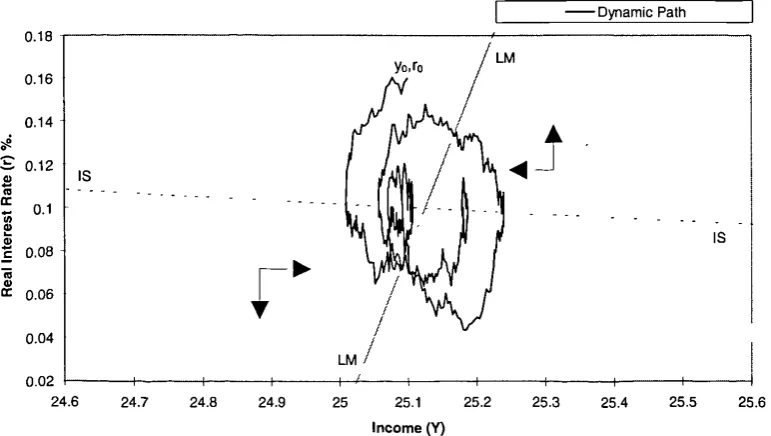
Given the link between the reduced form model for the state variables r and x and the
underlying economic model variables r and y, it is useful to view the system in the
economic framework. Figure 2-5 and Figure 2-6 show the solution path in the IS-LM
framework. The IS schedule represents the line, along which, the goods market is in
equilibrium. For all points on the line dy I dt = 0. The LM schedule represents the line,
along which, the money market is in equilibrium. For all points on the LM schedule,
dr' dt = 0 .
0.02 0.18
0.16
0.14
IS S 0.12
cc 0.1
c 0.08
cc 0.06
0.04
IS
IS
IS 0.16
0.14
0.1
c 0.08
•
C)
cc 0.06
0.04
0.02
TICE (1998) DYNAMIC MEAN INTEREST RATE MODELS AND THE IS-LM FRAMEWORK
- Dynamic Path
24.6 24.7 24.8 24.9 25 25.1 25.2 25.3 25.4 25.5 25.6
Income (Y)
FIGURE 2-5: THE DYNAMICS OF THE SOLUTION PATH IN THE IS-LM FRAME 6,-=0.025, CY,=0
- Dynamic Path 0.18
24.6 24.7 24.8 24.9 25 25.1 25.2 25.3 25.4 25.5 25.6
[image:34.595.109.495.58.276.2]Income 01
FIGURE 2-6: THE DYNAMICS OF THE SOLUTION PATH IN THE IS-LM FRAME Gr=0, CT0
Monetary authorities may influence economic variables by either fiscal or monetary
means4. In the IS-LM framework fiscal policies determine the value of the parameter a
which is assumed to incorporate taxes and government expenditure, 5 and monetary
4 With suitable caveats, a closed economy is assumed, for instance.
policies determine the value of the parameter m, so a and ms may each be time
dependent. Since 1.t depends upon a and m„ a direct economic justification for allowing
p. to be time varying can be supplied. Later, after the full model is introduced in
chapter 3, alternative methods of interest rate control shall be suggested that may be
available to the monetary authorities.
2.5 Conclusions
It has been seen how an economically motivated model, capable of producing
complex dynamics deterministically may describe the short rate process. Furthermore,
the model can be thought of as generalising several popular models in the interest rate
literature. The capability of the model to describe business cycle behaviour without
recourse to complex volatility functions is not without motive. The economic model,
describing the interaction of the product and money markets in the economy, exhibits
this behaviour endogenously for realistic parameter values. It is also the case that
economic meaning can be ascribed to the reduced form parameters of the model (2.3-5)
with reference to the underlying economic framework. In chapter 3 it will be seen how
this model may be extended to allow more complex types of behaviour. Chapters four
3.1 Introduction
This chapter investigates a particular three factor model which, for realistic
parameter values, exhibits chaotic behaviour. The three factor model arises naturally as
an extension to the economically derived two factor model, shown in chapter two. The
implications of its chaotic behaviour are analysed. The emphasis is concentrated on the
ability of the three factor model to forge large scale deterministic dynamics. External
noise serves only a minimal role in the overall dynamics. It is shown that the three
factor model can replicate features of empirical interest rate processes such as business
cycles and certain properties of term structures.
The chapter proceeds as follows. Section 3.2 describes an economic argument for
the third factor, p, to vary. Its dynamics are motivated on behavioural grounds. A
resultant three factor model is found. This then proves to be a further generalisation of
the two factor model (2.3-5). The model is consistent with the description of dynamic
mean models in (2.2-1). Section 3.3 discusses the implications of the form of the three
factor model. It is shown that it can exhibit chaotic behaviour for realistic parameter
values. Under certain transformations the model is equivalent to the Lorenz equations,
the dynamics of which are well documented. One desirable property is shown to be that
the system is bounded by the region of the attractor. The dynamics in the absence of
noise are discussed, motivating a very simple form for the volatility functions. Section
3.4 discusses a variety of estimation and pricing issues for the model. It is shown how
term structures may be obtained with a wide variety of behaviour. Bond pricing is
discussed and sensitivity analysis over parameter values is presented. Discussion is
made regarding the reconstruction of the attractor via principal component analysis and
an empirical investigation is given, showing the existence of an attractor qualitatively
similar to Lorenz. Due to the chaotic nature of the system, the stochastic version is
is constant. However, in practice
TICE (1998) A THREE FACTOR MODEL
structures are found to be comparable. Section 3.4.2 discusses how the underlying
economics of the model may imply methods for policy control of the system. Section
3.5 concludes.
3.2 Extending the two factor model
In the two factor model (2.3-5), p represents the influence of r upon the prospective
level of interest rates, x. It measures the degree of feedback between r and the rest of
the economy. In the derivation of (2.3-5) it was assumed that parameter values were
constant, so that p= b k
a, (1—
c)1—c u +a y bklu
parameter values, and hence the value of p, are determined by the aggregate behaviour
of individuals operating within the economy. As economic activity takes place it is
likely that the realised value of p will not be constant. Since a y is small compared to
oc„, it is the case that p= —b —k < O. Macroeconomic interpretations of the 1— c u
parameters in this equation are discussed in chapter two. Here the interpretation is that
p is related to the availability of transactions credit within the economy, via the
parameter k. From the discussion in chapter two, it is was assumed that k would take on
only positive values. However, economic arguments for extending the range of values
that k may take on is present in the literature (for example Dornbusch and Fischer
(1994), or Black and Dowd (1994)). If transaction credit is not used then k is positive.
If transaction credit is available and used extensively then it is supposed that k may be
negative, and hence p may be positive.
Under the supposition that k and hence p may be time varying it is necessary to
model the dynamics of p. Taking equations (2.3-5) as given define
dp =7(T) — p)dt +apdzp 7 > 0, (3.2-1)
where is the equilibrium value of p and 7 is the reversion rate of p towards 17, . This
justification for the assumption of dynamics of the form (3.2-1) is not given, but one
may suppose that as individuals become aware that the realised value of p is not in some
utility maximising equilibrium, they modify their behaviour so that p is brought closer
to an optimal value. An implication is that p would not revert quickly towards /5.
Rather, it would move relatively slowly as the value of p was revealed.
It is supposed that 13 is a function of r and x. Expand 17 (r,x) in a Taylor's series
expansion about the fixed point at ro = xo= p to obtain
(r,x)= 101,17 1)+ T r( r — 1-0+ Tx(x—l-t)+ 1 Trr(0 r-1- 2 +.1T3 (x - 02 T
+Il xr(x - I-0( r — II)±. —
(3.2-2)
where subscripts denote partial differentiation. It is desirable to ensure that with
suitable choices of parameters r does not grow arbitrarily small or arbitrarily large. It
has been seen that when p > 1 the system (2.3-5) goes to -± 0. (unless it lies initially on
the separatrix taking it to the fixed point). Here, p represents the use of credit in the
economy and an economic argument can be used to determine its behaviour. It can be
expected that when both r and x, and hence r and y, are large relative to p, credit is
both costly and not needed, and p is small or negative. Conversely, when both income
and interest rates are low relative to p, despite the small cost of credit, individuals are
either unwilling or unable to use credit so p is again small or negative. If both income
and rates are at middle levels then credit is used. When income is high and rates are
low then credit is used extensively and p may be large. However, if income is low but
rates are high then credit is still used extensively. In the context of the system (2.3-5)
the interpretation is for the use of credit in anticipation of interest rates decreasing.
This provides the appropriate minimal behaviour, and may be expressed by setting
TICE (1998) A THREE FACTOR MODEL
where 8 = T)(141), -0 = 17„ evaluated at 040, and the other derivatives have been
set to zero. The form of (3.2-3) ensures that if both x and r are large or if both x and r
are small, relative to ti, then p becomes small. If this happens then x begins to revert
more strongly to i_t than to r. Since r reverts to x, r will also begin to move back
towards ti. Note that if only one of x and r is large, with the other small relative to i.t, r
will tend to increase if it is small and decrease if it is large. The behaviour of p does not
need to be specified in this situation.
In effect, the form of (3.2-3) means that the Taylor series expansion (3.2-2) is
truncated in a second order approximation.. However, the equations for r and x were
obtained from the affine IS-LM system. A fully comparable system might require the
development of a second order version of IS-LM. Such a system is not considered here,
although one could be embedded within the framework of (2.2-3). It is the case that
(2.3-5) can be regarded as a special case of a higher order approximation.' Note also
that a purely first order approximation for T) would give a three factor affine system.
The dynamics of such systems (in the absence of noise) are well understood. The
behaviour of r could be considered to be qualitatively similar to its behaviour in the two
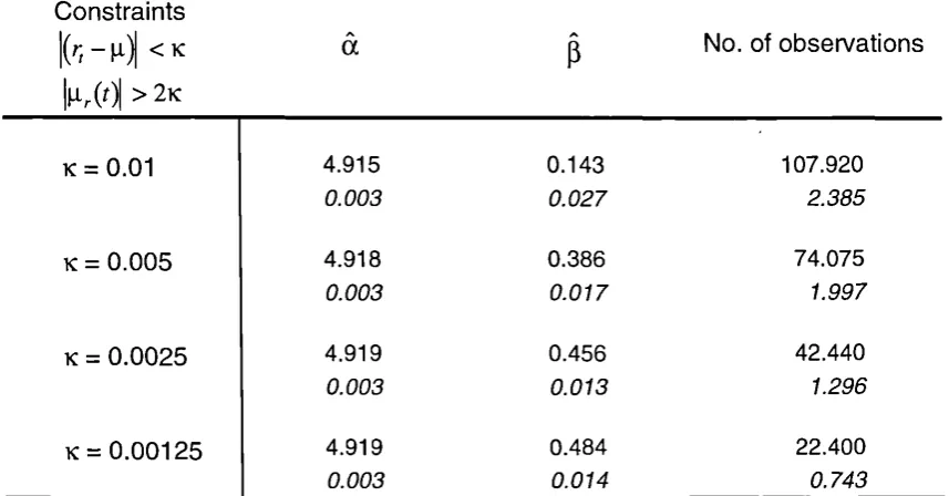
factor system (2.3-5).
In the analysis of the model performed below it shall be seen that p, and hence k,
cycles from positive to negative values over a period of a number of years. 2 This may
be interpreted as a series of credit booms and credit squeezes.
The complete three factor system is thus
'It is anticipated that the dynamics of a higher order approximation would not be less complex than those of the affine system presented here.
(3.3-1) dr = a(x — r)dt + rdz,
= 13(pr + (1— p)Ji—x)dt + crxdz, dp = y(.5 — cqx — ii)(r — p)dt + pdzp
(3.2-4)
with a large and 1 and y relatively small, and the values of 5 and 4) yet to be
considered. (3.2-4) is consistent with the definition (2.2-1) of a dynamic mean term
structure model.
3.3 Assessing the dynamics of the model; the relation to Lorenz
The nature of the system (3.2-4) can be clarified by introducing a change of
variables. For the moment, to lay bare the underlying dynamics, it is supposed that the
volatility terms are identically zero so that the system is deterministic. Set
where s
Il
YOWith the assumption of zero volatilities this transforms (3.2-4) into the following
system:
dX = a(Y — X)dt
dY =13(5X — ZX — Y)dt
dZ = (XY — yZ)dt
(3.3-2)
With f3 = 1 this is the Lorenz system 3 . The Lorenz system has been widely studied,
for instance see Sparrow (1982) and the references therein. For suitable values of the
parameters a, 5 and y it exhibits chaotic behaviour: starting the evolution of the system
from two points initially close together will produce trajectories that locally diverge
exponentially while globally remaining within a bounded region. For instance, Figure
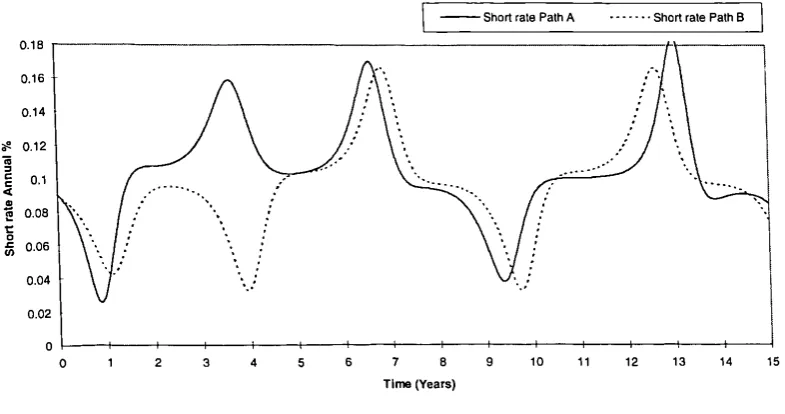
Short rate Path B - Short rate Path A
TICE (1998) A THREE FACTOR MODEL
3-14 shows the evolution of r under two different starting conditions Path (A) has
initial values (r,x,p) = (0.09, 0.085, 10) and path (B) has initial values (r,x,p) = (0.09,
0.085, 5). The paths diverge rapidly.5 For general introductions to chaotic systems see
Hilbom (1994) or Marek and Schreiber (1991), amongst others.
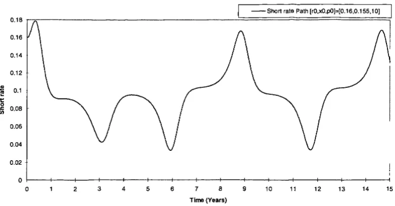
0 2 3 4 5 6 7 B 9 10 11 12 13 14 15
[image:42.595.101.494.166.373.2]Time (Years)
FIGURE 3-1: THE EVOLUTION OF r
In recent years there has been considerable interest in searching for non-linear and
chaotic features in financial and economic time series. For instance stock market data
has been examined by Abhyankar, Copeland and Wong (1997), Scheinkman and
LeBaron (1992) and Hsieh (1991), and many others. For a recent review article see
LeBaron (1994). Many authors attempt to uncover non-linear structure by applying one
of a standard set of tests, such as the BDS test (Brock at al. (1986)) or the
Grassberger-Procaccia test (1983). Barnett et al. (1995) provide a comparison of a number of tests
applied to US money supply data. Fewer papers have investigated interest rate data for
chaotic features. Authors who have studied T-bill data include Brock (1988), who
found a correlation dimension of two, and Larrain (1991) who fitted a particular
non-4 Numerical integration was performed using four step Runge-Kutta.
linear econometric model to the data. McNevin and Neftgi (1992) investigate various
time series including T-bill and bond returns.
There are also comparatively few attempts to devise non-linear and chaotic models.
Examples are Goodwin (1990), de Grauwe, Dewachter and Ernbrechts (1993), and
Medio and Gallo (1992), amongst others. Goodwin explores a number of chaotic
systems in economics, chiefly focusing on situations describable by the ROssler system.
Chaos and business cycles have attracted some attention, for instance Brock and Sayers
(1988).
A number of interest rate models incorporate some non-linearity. These include
square Gaussian models (Jamshidian (1993)) and the Black-Karasinski (1991) model in
which the short rate is a non-linear function of Gaussian state variables. Other models
such as Longstaff (1992) and Platten (1994) incorporate non-linear terms into the drift
of the short rate. Ait-Sahalia (1996) conducts an empirical investigation of Eurodollar
deposit rates and concludes that the drift of the short rate is strongly non-linear. Stanton
(1997), in a similar investigation using Treasury bill data reaches the same conclusion.
As far as I am aware the current research presents the first example of a naturally
derived non-linear model of interest rates exhibiting chaotic behaviour.
Another characteristic of the Lorenz system is also apparent in Figure 3-1. r has two
ranges about which it fluctuates. Either it is oscillating with high values, greater than
[t., or it is oscillating with low values, less than ii. This can be seen more clearly in
Figure 3-2. This is a graph of the values of r and p as path (A) evolves. It is clear that
the path loops around one of two lobes, switching from time to time from one lobe to
the other. The parameters are such that switches from one regime ('high rates') to the
TICE (1998) A THREE FACTOR MODEL
C
0.132
Short Rate
FIGURE 3-2: THE AT 1 RACTOR IN (r,p) SPACE
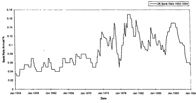
Figure 3-3 shows UK interest rates between 1954 and 1994. Although it is unlikely
that a single stationary economic model would explain interest rate behaviour over this
period, nevertheless there is some evidence from the figure that interest rates fall into a
'business cycle' pattern, moving from higher to lower levels and back on average every
five years, or so. Figure 3-3 may be compared with Figure 3-4, obtained using
illustrative parameter values. In both Figure 3-3 and Figure 3-4 interest rates are
initially fluctuating at low levels. There is a sudden transition to a high rate regime,
that temporarily dips back to low rates part way through. Figure 3-4 was not found
through an estimation procedure, but it illustrates that the range of possible behaviours
of (3.2-4) does not exclude histories qualitatively similar to the realised short rate time
0.18 —
0.16
0.14
, 0.12
i
0060.04
t
I —UK Bank Rate 1954-1994!
1
0.02
0
Jan 1954 Jan 1958 Jan 1962 Jan 1966 Jan 1970 Jan 1974 Jan 1978 Jan 1982 Jan 1986 Jan 1990 Jan 1994
[image:45.595.95.481.53.256.2]Date
FIGURE 3-3: UK INTEREST RATE 1954-1994
I — Short Rate Path I
0 2 4 6 8 10 12 14 16 18 20 22 24 26 28 30 32 34 36 38 40
Time (Years)
FIGURE 3-4: AN ILLUSTRATIVE EVOLUTION OF r
The behaviour of orbits in the Lorenz system (3.3-2) is highly complex, and is
sensitive to the values of its parameters and to the initial state. When the parameter 8 is
less than 1 the system has a single fixed point at
X=Y=Z= 0
All paths converge to this fixed point, which corresponds to
r = x = p,, p=
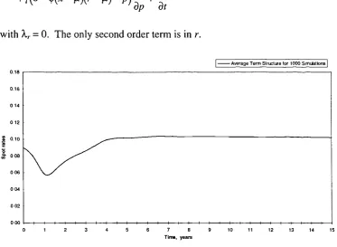
![FIGURE 3-15: TERMINAL VALUES FOR r: x0 IN THE RANGE [0.02,0.18]](https://thumb-us.123doks.com/thumbv2/123dok_us/9846381.485810/62.595.92.493.53.258/figure-terminal-values-r-x-range.webp)