WORKING PAPERS SERIES
WP07-03
Equilibrium Return and Agents'
Wealth Selection in a Financial Market
with Heterogeneous Agents
∗
Mikhail Anufriev
a,b,†Pietro Dindo
b,a,‡a CeNDEF, Department of Quantitative Economics, University of Amsterdam, Roetersstraat 11, NL-1018 WB Amsterdam, Netherlands
b LEM, Sant’Anna School of Advanced Studies, Piazza Martiri della Libert´a 33, 56127 Pisa, Italy
December 11, 2007
Abstract
We study the co-evolution of asset prices and agents’ wealth in a financial market populated by an arbitrary number of heterogeneous, boundedly rational investors. We model assets’ demand to be proportional to agents’ wealth, so that wealth dynamics can be used as a selection device. For a general class of investment behaviors, we are able to characterize the long run market outcome, i.e. the steady-state equilibrium values of asset return, and agents’ survival. Our investigation illustrates that market forces pose certain limits on the outcome of agents’ interactions even within the “wilderness of bounded rationality”. As an application we show that our analysis provides a rigorous explanation for the results of the simulation model introduced in Levy, Levy, and Solomon (1994).
JEL codes: G12, D84, C62.
Keywords: Heterogeneous agents, Asset pricing model, Bounded rationality, CRRA framework, Levy-Levy-Solomon model, Evolutionary Finance.
∗Preliminary results of this study have been presented in a Symposium on Agent-Based Computational
Methods in Economics and Finance, Aalborg, September 2006 and published in the Symposiums’ proceedings
Advances in Artificial Economies, ed. by C. Bruun, pp. 269–282, Springer Verlag, under the title “Equilibrium return and agents’ survival in a multiperiod asset market: Analytic support of a simulation model”. We wish to thank all the participants of the Symposium and of the seminars in Amsterdam, Marseille, Paris and Sydney for useful comments and stimulating questions. We especially thank Buz Brock, Doyne Farmer and Moshe Levy for reading earlier drafts of the paper and providing very detailed comments. Mikhail Anufriev kindly acknowledges the joint work with Giulio Bottazzi without which this paper would not be written. We acknowledge financial support from the E.U. STREP projects FP6-2003-NEST-PATH-1 and FP6-012410. The usual exemption applies.
1
Introduction
Consider a financial market where a group of heterogenous investors, each following a different strategy to gain superior returns, is active. The open question is to specify which agents will survive in the long run and how agents’ interaction affects market returns. This paper seeks to make a contribution in this direction.
At this purpose we investigate the co-evolution of prices and agents’ wealth in a stylized market for a long-lived financial asset, populated by an arbitrary number of heterogenous agents. Agents decide, period after period, which fraction of their wealth to invest in the financial asset. Their investment decisions are modeled in a general manner, as some smooth functions of past realizations of prices and dividends. An important feature of our model is that the dynamics of price and wealths are closely intertwined. In fact, agents impact market prices proportionally to their relative wealth, and, at the same time, market price realizations determine agents’ wealths. In other words, the dynamics of price and wealths acts naturally as a selection device operating on the set of different investment strategies, while, at the same time, the successful strategies determine the price and wealth dynamics.
By focusing on the asset price dynamics in a market with heterogeneous agents, our paper clearly belongs to the growing field of Heterogeneous Agent Models (HAMs), see Hommes (2006) for a recent survey. We share the standard set-up of this literature and assume het-erogeneous investors to decide whether to invest in a risk-free bond or in a risky financial asset.1 In the spirit of Brock and Hommes (1997) and Grandmont (1998) we consider
stochas-tic dynamical system and analyze the sequence of temporary equilibria of its determinisstochas-tic skeleton. As opposed to the majority of HAMs, which consider only a few types of investors and concentrate on heterogeneity in expectations, here we develop a general framework which can be applied to a quite large set of investment strategies, so that heterogeneity with respect to risk attitude, expectations, memory and optimization task can be accommodated. In fact, we characterize long run behavior of asset prices and agents’ wealth distribution for a general set of competing investment strategies.
An important feature of our model concerns the demand specification. Many HAMs (see e.g. Brock and Hommes (1998); Gaunersdorfer (2000); Brock, Hommes, and Wagener (2005)) employ the setting where agents’ demand is not changing with wealth, i.e. exhibits constant absolute risk aversion (CARA). In contrast, we assume that demand increases linearly with agents’ wealth, which corresponds to the so-called constant relative risk aversion (CRRA) property. An advantage of this approach is that wealth dynamics acts as a selection mecha-nism and thus determines long run survival. On the contrary, in CARA models a selection mechanism has to be introduced ad hoc time by time. Furthermore, experimental literature seems to lean in favor of CRRA rather than CARA (see e.g. Kroll, Levy, and Rapoport (1988) and Chapter 3 in Levy, Levy, and Solomon (2000)).
The analytical exploration of the CRRA framework with heterogeneous agents is difficult, because the wealth dynamics of every agent have to be taken into account. Despite this obstacle, the recent papers of Chiarella and He (2001, 2002), Anufriev, Bottazzi, and Pancotto (2006), Anufriev and Bottazzi (2006) and Anufriev (2008) make some progress. In particular, the last studies introduce a geometric tool, so-called Equilibrium Market Curve (EMC), which can be used to carry out the equilibrium analysis. All these studies, however, are based on the assumption that the price-dividend ratio is exogenous. This seems at odd with the
1Recently, also some models with heterogeneous agents operating in markets with multiple assets (Chiarella,
standard approach, where the dividend process is exogenously set, while the asset prices are endogenously determined. In our paper we overcome this problem, and use the EMC approach to analyze a market for a financial asset whose dividend process is exogenous, so that the price-dividend ratio is a dynamic variable.2
The CRRA setup with exogenous dividend process allows us to link our model with agent-based simulations, and in particular with one of the first agent-agent-based model of a financial market introduced in Levy, Levy, and Solomon (1994) (LLS model, henceforth). Their work investigates whether some stylized empirical findings in finance, such as excess volatility or long periods of overvaluation of asset, can be explained by relaxing the assumption of a fully-informed, rational representative agent. Despite some success of the LLS model in reproducing the financial “stylized facts”, all its results are based on simulations. Our general setup can be applied to the specific demand schedules used in the LLS model, and, thus, provides an analytical support to its simulations.
As we are looking at agents’ survival in a financial market ecology, our work can be classified within the realm of evolutionary finance. A seminal work of Blume and Easley (1992), as well as more recent papers of Sandroni (2000), Hens and Schenk-Hopp´e (2005), Blume and Easley (2006) and Evstigneev, Hens, and Schenk-Hopp´e (2006), investigate how beliefs about the dividend process affect agents’ dominance in the market. There are two main differences of our work with this literature. First, whereas their work focuses on portfolio selection, we focus on relating asset returns in terms of the risk-free rate. Indeed, in their model an investor can choose among a number of different risky assets, while in our model agents can invest either in a risky or in a riskless asset. Second, although these contributions assume that each investment strategy depends on the realization of exogenous variables, i.e. dividends, our investors can also condition on past values of endogenous variables such as past prices. As a consequence in our framework prices today influence prices tomorrow through their impact on the agents’ demands. This is important especially when the stability of the surviving strategy is investigated. In fact, when the investment strategy is too responsive to price movements, fluctuations are typically amplified and unstable price dynamics are produced. Indeed, we show that local stability is related to how far agents look in the past.
This paper is organized as follows. Section 2 presents the model and leads to the definition of the stochastic dynamical system where prices and wealths co-evolve. Section 3 studies the equilibria of the deterministic version of the dynamical system and introduces the tools to investigate their stability. Section 4 applies the general model to the special case where agents are mean-variance optimizers and explains the simulation results of the LLS model. The analysis of the general model is completed in Section 5, while Section 6 summarizes our main results and concludes. Proofs are collected in Appendices at the end of the paper.
2
The model
Let us consider a group of N agents trading in discrete time in a market for a long-lived financial asset. Assume that the asset is in constant supply which, without loss of generality, can be normalized to 1. Agents can lend the share of wealth which is not invested in the financial asset in return of an exogenously given constant interest rate rf > 0 per period,
i.e. they can buy a risk-less asset. This asset serves as num´eraire with price normalized to 1
2Recent model of Chiarella, Dieci, and Gardini (2006) is another example of the HAM built in the CRRA
in every period. The financial (risky) asset pays a dividend Dt at every time t in units of the
num´eraire, while its price Pt is fixed through market clearing.
Let Wn,t stand for the wealth of agent n at time t. It is convenient to express agent’s
demand for the risky asset in terms of the fractionxn,t of wealth invested in this asset, so that
agent n invests an amountxn,tWn,t in the risky asset at time t. If the dividend is paid before
trade takes place, wealth of agent n evolves as
Wn,t+1 = (1−xn,t)Wn,t(1 +rf) +xn,tWn,t
Pt+1+Dt+1 Pt
, (2.1)
where the price at time t+ 1 is fixed through the market clearing condition
!N n=1
xn,t+1Wn,t+1 Pt+1
= 1. (2.2)
In this system prices and wealth co-evolve because the price depends on the current agent’s wealth via (2.2) and, at the same time, the wealth of every agent depends on the contempora-neous price via (2.1). Before deriving the solutions of these equations, we devote our attention to the individual investment decisions xn,t.
2.1
Investment Functions
We intend to study the evolution of the asset price and agents’ wealth under an investment strategies as general as possible. Therefore, we avoid any explicit formulation of the demand and suppose that the investment shares xn,t are general functions of past realizations of prices
and dividends. Following Anufriev and Bottazzi (2006) we formalize this intuitive concept of investment strategy as an investment function.
Assumption 1. For each agent n = 1, . . . , N there exists an investment function fn which
maps the information set, containing realized dividends and prices, into an investment share:
xn,t =fn
"
Dt, Dt−1, Dt−2, . . .;Pt−1, Pt−2, . . .
#
. (2.3)
Agents’ investment decisions evolve following individual prescriptions. Notice that since the investment choices should be made before the trade starts, the information set contains all the past dividends up to Dt, and all the past prices up to Pt−1.
Assumption 1 leaves a high freedom in the demand specification. The only essential restric-tion is that the investment share does not depend on the contemporaneous trader’s wealth. This implies that the demand for the risky asset is linearly increasing with the trader’s wealth. In other words, ceteris paribus investors maintain a constant proportion of their invested wealth as their wealth level changes. Such behavior can be referred as a constant relative risk aversion (CRRA) framework.3
A number of standard demand specifications are consistent with Assumption 1. In Sec-tion 4.1, as an applicaSec-tion, we consider agents who maximize mean-variance utility of their next period expected return. Other investment behavior can also be accommodated within our framework, for instance, one can consider agents behaving in accordance with the prospect theory of Kahneman and Tversky (1979).4
3The distinction between constant relative and constant absolute risk aversion (CARA) behavior was
in-troduced in Arrow (1965) and Pratt (1964), who also relate these concepts with utility maximization. Under CARA framework agents maintain a constant demand for the risky asset as their wealth changes.
The generality of the investment functions allows modeling the agents’ forecasting prac-tice with a big flexibility too. The formulation (2.3) includes as special cases both technical trading, when agents’ decisions are driven by the observed price fluctuations, and more fun-damental attitudes, e.g. when the decisions are made on the basis of the price-dividend ratio. It also includes the case of constant investment strategy, occurring when agents assume the stationarity of the ex-ante return distribution.
Despite high flexibility, our setup does not include a number of important behavioral rules of agents. Since the current wealth is not included as an argument in the investment function, all the demand functions of CARA type are not covered by our framework. Also the current price is not among the arguments of (2.3). Therefore, investors deriving their investment share conditional on the (hypothetical) current price cannot be reconciled with our setup.
2.2
Co-evolution of Wealth and Prices
Given the asset price and agents’ wealths at time t together with the dividend and agents’ investment strategies at t+ 1, prices and wealth at t+ 1 are simultaneously determined by the evolution of wealth (2.1) and by the market clearing condition (2.2). To obtain an explicit solution forPt+1, and thereafterWt+1, we can use (2.1) to rewrite the market clearing equation
(2.2) as
Pt+1 = N
!
n=1
xn,t+1Wn,t
$
(1−xn,t)(1 +rf) +xn,t
%Pt+1
Pt
+ Dt+1
Pt
&'
.
The solution of this equation with respect to Pt+1 gives
Pt+1 =
(N
n=1xn,t+1Wn,t
%
(1−xn,t)(1 +rf) +xn,tDPt+1t
&
1− 1 Pt
(N
n=1Wn,txn,t+1xn,t
. (2.4)
Wealth evolution (2.1) then determines individual wealth Wn,t+1 for every agent n. The
resulting expressions can be conveniently written in terms of the price return and dividend yield defined, respectively, as
kt+1 = Pt+1
Pt −
1 and yt+1 = Dt+1
Pt ,
as well as in terms of agents’ relative wealth
ϕn,t=
Wn,t
(
mWm,t .
Dividing both sides of (2.4) by Pt and using that Pt =(xn,tWn,t, one derives the evolution
of price returns. Together with the resulting expression for the evolution of wealth shares, it gives the following system:
kt+1 =rf +
(
n
"
(1 +rf) (xn,t+1−xn,t) +yt+1xn,txn,t+1
#
ϕn,t
(
nxn,t(1−xn,t+1)ϕn,t
,
ϕn,t+1 =ϕn,t
(1 +rf) + (kt+1+yt+1−rf)xn,t
(1 +rf) + (kt+1+yt+1−rf) (mxm,tϕm,t
, ∀n ∈{1, . . . , N}.
According to the first equation, the return depends on the totality of agents’ investment decisions for two consequent periods. High investment fractions for the current period tend to increase the current price and, hence, the return. This effect is due to an increase of current demand. Moreover, the effect of agents’ decision on the price return is proportional to their relative wealth. The second equation in (2.5) shows that the relative wealth of every agent changes according to the agent’s relative performance, where the return of each individual wealth should be taken as performance measure.
2.3
Dividend Process and Dynamical System
The last ingredient of the model is the dividend process. The previous analytical models built in the CRRA framework, such as Anufriev, Bottazzi, and Pancotto (2006), Anufriev and Bottazzi (2006) and Anufriev (2008), assume that the dividend yield is an i.i.d. process. This assumption implies that any change in the level of price causes an immediate change in the level of dividends. In reality, however, the dividend policy of firms is hardly so fast responsive to the performance of the firm’s assets, especially when prices are driven up by speculative bubbles. In this paper we consider the alternative setting, where the dividend process is completely exogenous with respect to the financial market.
Assumption 2. The dividend realization follows a geometric random walk,
Dt=Dt−1(1 +gt), (2.6)
where the growth rate, gt, is an i.i.d. random variable.
Rewriting this assumption in terms of dividend yields and price returns we get
yt+1 =yt
1 +gt+1
1 +kt
. (2.7)
Equations (2.5) and (2.7) together with the investment functions (2.3), rewritten as functions of price returns and dividend yields, specify the evolution of the asset-pricing model with N
heterogeneous agents.
3
Equilibrium Returns and Agents’ Survival
The dynamics of our model is stochastic due to the fluctuations of the dividend process. Fol-lowing the typical route in the literature (cf. Brock and Hommes (1997), Grandmont (1998)), we start from the analysis of thedeterministic skeleton of this stochastic dynamics. The skele-ton is obtained by fixing the growth rate of dividends in (2.6) at the constant level g > −1. Our simulations, discussed later in this paper, show that the local stability analysis of the de-terministic skeleton gives considerable insight for the case when the growth rate of dividends is a random variable.5
Before we start, let us introduce the investment decision weighted with relative wealth as
-xt
.
s = N
!
n=1
xn,tϕn,s, (3.1)
5It is important to keep in mind that the agents do take the risk due to randomness into account, when
where the time of the decision, t, and the time of the weighting wealth distribution, s, can be different. The deterministic skeleton for N agents whose investment functions depend on the lagged price returns and dividend yields6 can be then written as
xn,t+1 =fn
"
kt, kt−1, . . . , kt−L+1;yt+1, yt, . . . , yt−L+1
#
, ∀n∈{1, . . . , N}
ϕn,t+1 =ϕn,t
(1 +rf) + (kt+1+yt+1−rf)xn,t
(1 +rf) + (kt+1+yt+1−rf)
-xt
., ∀n∈{1, . . . , N}
kt+1 =rf +
(1 +rf)
-xt+1−xt
.
t+yt+1
-xtxt+1
.
t
-xt(1−xt+1)
.
t
,
yt+1 =yt
1 +g
1 +kt .
(3.2)
Given the arbitrariness of the size of population N, of the memory span L, and the absence of any specification for the investment functions, the analysis of dynamics generated by (3.2) is highly non-trivial in its general formulation. However, as we show in Section 3.1, the constraints on the dynamics set by the dividend process, the market clearing equation and the wealth evolution are sufficient to (i) uniquely characterize the steady-state equilibrium level of price returns, (ii) describe the corresponding possible distributions of wealth among agents, and (iii) restrict the possible values of steady-state equilibria dividend yields to a well specified set. Furthermore, in Section 3.2 we derive general conditions under which convergence to these equilibria is guaranteed.
The primary issue is whether, when the variables are restricted to the set of economically relevant values, the dynamics is well specified. In particular, the requirements of positive prices and positive dividends imply, respectively, that the price returns should exceed−1 and the dividend yield should be larger than zero. The following result shows that under such restrictions and when, in addition, agents are not taking short positions in both assets, the dynamics in (3.2) can always be described by a well-defined dynamical system.
Proposition 3.1. Assume that agents do not take short positions in both the risk-less and the
risky assets. In other words, given investment functions fn as defined in Ass. 1, assume that
the image of fn belongs to (0,1) for every n. (3.3)
Then the system (3.2)defines a2N+2L-dimensional dynamical system of first-order equations.
The evolution operator associated with this system
T(x1, . . . , xN;ϕ1, . . . ,ϕN;k1, . . . , kL;y1, . . . , yL) (3.4)
is well-defined on the set
D= (0,1)N ×∆N ×(−1,∞)L×(0,∞)L, (3.5)
consisting respectively of investment sharesxn, wealth shares ϕn, price returns kl and dividend
yields yl, where n = 1, . . . , N and l = 1, . . . , L, and ∆N denotes the unit simplex in N
-dimensional space
∆N =
/
(ϕ1, . . . ,ϕN) :
!N
m=1ϕm = 1, ϕm ≥0 ∀m
0
.
6In order to deal with a finite dimensional dynamical system, we restrict the memory span of each agent
Proof. We prove that the dynamics from D to D is well-defined. The explicit evolution operator T, which is used in the stability analysis, is provided in Appendix A.
Let us start with period-t variables belonging to the domain D and apply the dynamics described by (3.2) to them. Since kt > −1, the fourth equation is well define and yt+1 is
positive. As a result, the first equation defines the new investment shares belonging to (0,1) in accordance with the assumption in (3.3). It, in turn, implies that in the right-hand side of the third equation all the variables are defined, and the denominator is positive. Thus, kt+1
can be computed. Moreover, the denominator does not exceed 1, as a convex combination of numbers non-exceeding 1. Then, a simple computation gives
kt+1 > rf +
!
m
"
(1 +rf)(−1) + 0
#
ϕm,t =−1.
Finally, it is easy to see that both the numerator and the denominator of the second equation are positive and that (ϕm,t+1 = 1. Therefore, the dynamics of the wealth shares is
well-defined and takes place within the unit simplex ∆N.
In addition to proving the existence of a well-defined map7, this proposition also shows that
when the short position are forbidden, the agents’ wealth shares are bounded between 0 and 1. This makes sense because only short investment positions can give rise to a negative wealth for some agents. Throughout the remaining part of this paper we impose the no-short-selling condition (3.3).
3.1
Location of Steady-State Equilibria
In a steady-state, aggregate economic variables, such as price returns and dividend yields, are constant and will be denoted byk∗ andy∗, respectively.8 Every steady-state has also constant agents’ investment shares (x∗
1, . . . , x∗n), and wealth distribution (ϕ∗1, . . . ,ϕ∗n). Concerning the
latter we introduce the following definition.
Definition 3.1. In a steady-state equilibrium (x∗
1, . . . , x∗N;ϕ∗1, . . . ,ϕ∗N;k∗;y∗) an agent n is
said to survive if his wealth share is strictly positive, ϕ∗ n >0.
In every state of the economy there exists at least one survivor. In a steady-state withM
surviving agents (1 ≤ M ≤ N) we will always assume that the first M agents survive. The characterization of all possible steady-states of the dynamical system defined on the set D is given below.
Proposition 3.2. Steady-state equilibria of the dynamical system (3.2) evolving on the set D
exist only when the dividend growth rate g is larger than the interest rate rf.
Let g > rf and let (x∗1, . . . , x∗N;ϕ1∗, . . . ,ϕ∗N;k∗;y∗) be a steady-state of (3.2). Then:
- The steady-state price return is equal to the growth rate of dividends, k∗ =g;
- All surviving agents have the same investment share x∗#, which together with the
steady-state dividend yield y∗ satisfy
x∗# = g−rf
y∗+g−r f
. (3.6)
7With some abuse of language we usually refer to (3.2) and not to the first order mapT in (3.4) as “the
dynamical system”. The explicit map Twill be used only in the proofs.
8Notice that in the steady-state allLlagged values of the return and yield, which were introduced to define
Investment Share
Dividend Yield EMC
0 1
0 A
B
C
I II
Investment Share
Dividend Yield EMC
0 1
0
A
[image:10.595.78.527.84.238.2]I II
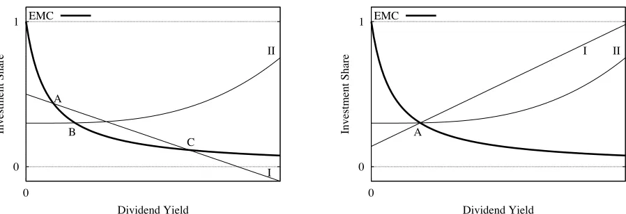
Figure 1: Location of equilibria forg > rf. Left panel: The Equilibrium Market Curve is shown with two investment functions, I and II. In total there are three intersections with the EMC,
corresponding to three different steady-states. In A and C agent I survives with ϕI = 1. In point
B agentII survives with ϕII = 1. The abscissa of a point gives the corresponding dividend yield, while the ordinate gives the investment share of the survivor. Right panel: When the investment functions are intersecting at some point belonging to the EMC, there exists a set of steady-states. All of them are given by A and have the same dividend yield and agent’s investment shares. However,
the wealth shares are arbitrary non-negative numbers satisfyingϕ1+ϕ2 = 1.
- The steady-state wealth shares satisfy
1
ϕ∗
m ∈(0,1] if m≤M
ϕ∗
m = 0 if m > M
and
M
!
m=1
ϕ∗m = 1. (3.7)
Proof. A proof obtained with a simple algebra is provided in Appendix B.
We have established that a steady-state can only exist when g > rf. This result begs
a question of what happens in the opposite case, when the dividend growth rate is smaller than rf. The answer on this questions will be postponed to Section 5. For the moment we
just assume that g > rf. Then many situations are possible, including the cases with no
steady-state, with multiple steady-states, and with different number of survivors in the same steady-state. Below we illustrate all these possibilities and discuss their economic implications. Above all notice that in all the steady-state equilibria the price grows with the same rate as the dividend. In contrast, the steady-state level of dividend yield depends on agents’ behaviors. Proposition 3.2 implies that the dividend yield, y∗, and the investment share of survivors, x∗
#, are determined simultaneously by (3.6). To find out how, let us introduce the
following definition.
Definition 3.2. The Equilibrium Market Curve (EMC) is the function
l(y) = g −rf
y+g−rf
defined for y >0. (3.8)
With this definition, since the investment share x∗
# is given by the value of the agent’s
investment function, (3.6) can be rewritten as the following system of M equations
l(y∗) =fm
"
The solutiony∗ is the dividend yield, andl(y∗) is the survivors’ investment share in the
steady-state. Condition (3.9) can be expressed graphically. Namely, all possible pairs (y∗, x∗#) can be found as the intersections of the EMC with the cross-section of the investment function of each survivor by the set
2
kt=kt−1 =· · ·=kt−L+1 =g; yt+1 =yt =· · ·=yt−L+1 =y
3
. (3.10)
We illustrate the use of the EMC in the left panel of Fig. 1 where a market with two agents is considered. Starting with arbitrary multi-dimensional investment functions, let us consider their cross-sections by the hyperplane (3.10). The resulting one-dimensional functions of the variable y are shown by the thin curves marked as I and II. Now draw the EMC (3.8) on the same diagram as a thick curve. According to (3.9), all possible steady-states of the dynamics are the intersections between the investment functions and the EMC. In this situation, obviously, there exist three steady-states. Point A corresponds to the case when (3.9) is satisfied for agent I. Therefore, in this steady-state he survives and, being alone, takes all available wealth, ϕ∗I = 1. The equilibrium dividend yield y∗ is the abscissa of point A, while the investment share of the survivor, x∗
I, is the ordinate of A. Finally, the equilibrium
investment share x∗
II of the second agent can be found as a value of his investment function at y∗. Notice that in this casex∗I > x∗II, which is important for stability as will become clear later. In the other two steady-states the variables are determined in a similar way. In particular, agent I is the only survivor at C, while at B only the second agent survives.
In all the steady-states in the left panel of Fig. 1 only one agent survives. Proposition 3.2 implies that the survival of more than one agent requires existence of a common intersection between their investment functions and the EMC. Such situation is illustrated in the right panel of Fig. 1. Every steady-state must have yield y∗ and average choicex∗# as determined by the coordinates of the pointA. However, any wealth distribution (i.e. all possible combinations of ϕI and ϕII satisfying to ϕI +ϕII = 1) defines some state. Generally, the
steady-states with multiple survivors, corresponding to the same point on the EMC, will form a manifold defined by condition (3.7). In all such steady-states the economic variables (return and yield) are the same, and the behavior of survivors must also be the same. Therefore, such equilibria may be indistinguishable when looking at the aggregate time series. However, the wealth shares of survivors can be different.
The EMC is an useful graphical tool which can be used to illustrate different long run possibilities arising under the dynamics of (3.2). It is, obviously, possible that the dynamics do not possess any steady-state (if no investment function intersects the EMC). It is also possible that the system possesses multiple steady-states with different levels of dividend yield (as in our first example), as well as multiple steady-states with the same level of yield (as in our second example). At the same time, the EMC shows that the often heard conjecture that, in the world of heterogeneous agents, “anything goes” is not necessarily valid. Even when the strategies of agents are generic, as in our framework, the market plays its role in shaping the aggregate outcome. The steady-states of system (3.2) can lie only on the EMC, which is a small subset of the original domain. The shape of the EMC is entirely determined by the exogenous parameters of the model, as g and rf, and does not depend on agents’ behavior.
asset. Indeed, the excess return in the steady-state according to (3.6) is given by
g+y∗−rf =
g−rf x∗
# ,
that is inverse proportional to the investment level x∗
#. However, every survivor takes exactly x∗
# of this excess return. We formulate it as the following
Corollary 3.1. At any steady-state equilibrium described in Proposition 3.2, the wealth return of each surviving agent is equal to g.
Thus, for survivors all the points in the EMC are welfare-equivalent. We stress, however, that different equilibria generally have different survivors.
3.2
Stability of Equilibria
In order to characterize the long-run dynamics of our financial market, we now turn to deriva-tion of the local stability condideriva-tions for the steady-states found in Proposideriva-tion 3.2. For this purpose we assume that all the investment functions entering in the dynamics (3.2) are dif-ferentiable with respect to their arguments.
3.2.1 Evolutionary selection of agents
The positive excess return earned in the steady-states allows the market to play the role of a natural selecting force. In fact, it rewards some agents at the expense of others, shaping in this way the long-run wealth distribution. The first part of our stability analysis focuses on this “natural selection” which operates on agents’ wealth shares. We show that some steady-states can be ruled out as unstable. The following general result holds.
Proposition 3.3. Consider the steady-state equilibrium "x∗
1, . . . , x∗N;ϕ∗1, . . . ,ϕ∗N;k∗;y∗
#
de-scribed in Proposition 3.2, where the first M agents survive and invest x∗#. It is (locally) stable if the following two conditions are met:
1) the investment shares of the non-surviving agents are such that
1−2 1 +g
g−rf < x
∗ m x∗
#
<1 ∀m∈{M + 1, . . . , N}. (3.11)
2) the steady-state "x∗
1, . . . , x∗M;ϕ∗1, . . . ,ϕ∗M;k∗;y∗
#
of the reduced system, obtained by eli-mination of all the non-surviving agents from the economy, is locally stable.
The system generically exhibits a fold bifurcation when the rightmost inequality in (3.11)
becomes an equality, and it exhibits a flipbifurcation if the leftmost inequality in (3.11)becomes an equality.
Proof. To derive the stability conditions, the (2N + 2L)× (2N + 2L) Jacobian matrix of
the system has to be computed and evaluated at the steady-state9. For the stability of the
system, the eigenvalues of this Jacobian should be inside the unit circle. In Appendix C we show that condition 1) is necessary and sufficient to guarantee that M eigenvalues of the Jacobian matrix lie inside the unit circle. Among the other eigenvalues there will beM zeros. Finally, all the remaining eigenvalues can be derived from the Jacobian associated with the “reduced” dynamical system, i.e. without non-surviving agents, evaluated in the steady-state. This implies condition 2).
9General references on the modern treatment of stability and bifurcation theory in discrete dynamical
Investment Share
Dividend Yield EMC
0 1
0 A
B
C
I II
Relative Slope, <f
!
> / l
!
Equilibrium Yield -1
-0.5 0 0.5 1
0 10 20
fold (any L)
flip (any odd L)
NS(1) NS(2)
[image:13.595.76.530.84.241.2]NS(2)
Figure 2: Stability conditions. Left panel: According to (3.11), the steady-state is stable (against the invasion by the non-survivors) if the non-survivors are less aggressive, i.e. their investment shares lie below the investment share of the survivors. Right panel: Stability of a steady-state when investment depends upon the average of past L total returns. In a stable steady-state for L = 1,
the pair "y∗,-f$(y∗ +g)./l$(y∗)# belongs to the dark-grey area. When L = 2 the stability region
expands and consists of the union of the dark- and light-grey areas. When L → ∞ the stability
region occupies all the space below “fold” line -f$(y∗+g)./l$(y∗) = 1. Crossing the border of the
stability region causes the corresponding type of bifurcation, where NS stands for Neimark-Sacker.
This proposition gives an important necessary condition for stability. Namely, the invest-ment shares of the non-surviving agents must satisfy (3.11). The leftmost inequality is always fulfilled for reasonable values of g and rf. The rightmost inequality shows that the survivors
should behave more “aggressively” in the stable steady-state, i.e. invest higher investment share than those who do not survive. This result is intuitively clear, because as long as the risky asset yields a higher average return than rf, the most aggressive agent has also the
highest total wealth return. For example, (3.11) implies the instability of equilibria B and C
in the left panel of Fig. 1. We illustrate it more thoroughly in the left panel of Fig. 2. In the stable equilibrium the investment shares of the non-surviving agents should belong to the gray area, i.e. lie below the investment shares of survivors.
Proposition 3.3 can be also viewed as a result about survival of some investment strategies against an “invasion” by other investment strategies, i.e.evolutionary stability. At the steady-state the dynamics is not affected by the agents who are not surviving, so that the non-survivors can be discarded from the analysis. Nevertheless, if a new, more “aggressive” investment strategy is introduced with an infinitely small fraction of wealth, it destroys the old equilibrium.
3.2.2 Stability of equilibrium with survivors
Consider the steady-state "x∗
1, . . . , x∗M;ϕ∗1, . . . ,ϕ∗M;k∗;y∗
#
and denote the vector of lagged returns and yields as e∗ = (k∗, . . . , k∗;y∗, . . . , y∗). In the notation below index m= 1, . . . , N
and index l= 0, . . . , L−1. Denote the derivative of the investment function fm with respect
to the contemporaneous dividend yield as fY
m, the derivative with respect to the dividend
yield of lagl+ 1 as fyl, and the derivative with respect to the price return of lagl+ 1 as fkl.
Furthermore, consistently with our previous notation, we introduce
-fY. =
M
!
m=1
ϕ∗mfmY(e∗), -fyl. =
M
!
m=1
ϕ∗mfyl
m(e∗),
-fkl.=
M
!
m=1
ϕ∗mfkl
m(e∗),
which are the weighted derivatives of investment functions evaluated in the steady-state. Fi-nally, we denote as l$(y∗) the slope of the Equilibrium Market Curve l(y) defined in (3.8) at
the steady-state equilibrium y∗.
The next proposition reduces the stability problem to the exploration of the roots of a certain polynomial.
Proposition 3.4. The steady-state "x∗
1, . . . , x∗M;ϕ∗1, . . . ,ϕ∗M;k∗;y∗
#
, described in Proposition
3.2, with M survivors is locally stable if all the roots of polynomial
Q(µ) = µL+1− 1 l$(y∗)
%-fY.µL+
L−1
!
l=0
-fyl.µL−1−l+ (1−µ)1 +g y∗
L−1
!
l=0
-fkl.µL−1−l
&
(3.12)
lie inside the unit circle. If, in addition, only one agent survives, then the steady-state is locally asymptotically stable.
The steady-state is unstable if at least one of the roots of polynomial Q(µ) is outside the
unit circle.
When the investment functions are specified, this proposition provides a definite answer to the question about stability of a given steady-state. One has only to evaluate the polynomial (3.12) in this steady-state and compute (e.g. numerically) all its L+ 1 roots.
Even in its general formulation, Proposition 3.4 allows us to get some insight about the determinants of stability. For example, when the investment strategies of all survivors are non-responsive to a change in the yield (i.e. all the derivatives of the investment functions are 0 in the steady-state), the expression in parenthesis becomes zero and the stability condition is obviously satisfied. Using a continuity argument, this also implies that the steady-state is stable if the relative average slopes of the investment functions are small enough with respect to the slope of the EMC.
Recall that in the case of many survivors (as depicted in the right panel of Fig. 1), there exists a set of steady-states corresponding to different distributions of wealth among survivors. Since the stability conditions depend on the partial derivatives of the investment functions weighted with the equilibrium relative wealth shares, some of the steady-states on the same manifold (i.e. with the same dividend yield and investment share) can be stable, while other can be unstable.
3.2.3 An example with investment conditioned on the total return
about total returns and not track its two separate components. Formally, assume that indi-vidual investment shares are given by
xn,t =fn
4
1
L L
!
τ=1
"
yt−τ +kt−τ
#5
. (3.13)
Simplifications in the polynomial (3.12) lead to
˜
Q(µ) = µL+1− 1 +µ+· · ·+µ
L−1
L
%
1 + (1−µ)1 +g
y∗
& (M
m=1fm$ (y∗+g)ϕ∗m
l$(y∗) . (3.14)
If all the roots of ˜Q(µ), evaluated in the corresponding steady-state, lie inside the unit circle, the dynamics is locally stable. From the results of Section 3.1 it follows that the equilibrium yield is given as a solution of l(y) =f(y+g). Thus, the last fraction in the polynomial (3.14) gives the relative slope of the “average” investment function of the survivors and the EMC at the steady-state.10
Proposition 3.3 and 3.4 give exhaustive characteristics of the stability conditions, but they are implicit. When L= 1 this requirement can be made explicit. Namely, the following result holds.
Corollary 3.2. Consider a steady-state of the system (3.2) with investment functions (3.13)
and lag L = 1, where all the non-survivors have been eliminated. The steady-state is locally
stable if
−y∗
1 +g+y∗ <
-f$(y∗+g). l$(y∗) <
y∗
y∗+ 2(1 +g). (3.15)
The steady-state generically exhibits flip or Neimark-Sacker bifurcation if the right- or
left-most inequality in (3.15) turns to equality, respectively.
Proof. This follows from standard conditions for the roots of second-degree polynomial to be
inside the unit circle. See appendix E for the details.
Conditions (3.15) are illustrated in the right panel of Fig. 2 in the coordinates (y∗,-f$./l$).
The steady-state is stable if the corresponding point belongs to the dark-grey area. From the diagram it is clear that the dynamics are stable for a low (in absolute value) relative slope
-f$./l$ at the steady-state.
How does the stability depend on the memory spanL? A mixture of analytic and numeric tools helps to reveal the behavior of the roots of polynomial (3.14) with higherL. The stability conditions for L = 2, derived in appendix E, can be confronted with the L= 1 case, see the right panel of Fig. 2. An increase of the memory span L brings stability to the system. With the next corollary we also prove that this is a general result.
Corollary 3.3. Consider a steady-state of the system (3.2) with investment functions (3.13). Provided that
-f$(y∗+g).
l$(y∗) <1, (3.16)
the corresponding steady-state is locally stable for high enough L.
10To be precise, recall that we use the one-dimensional cross-section, by the hyperplane (3.10), of a
To summarize, ifLis finite and low, the system can be stabilized by decreasing the average slope of survivors’ investment functions with respect to the slope of the EMC. Furthermore, if inequality (3.16) holds, an increase of memory span always stabilizes the system.
4
An example with Mean-Variance Optimizers
In this section we analyze the co-evolution of price returns, dividend yields and wealth shares for a specific set of the agents’ investment functions. We consider agents who are allocating wealth between the risky and the risk-less asset as to maximize their one period ahead mean-variance utility. We assume that agents’ expectations of future variables are computed using averages of past observations. Agents are heterogeneous in their degree of risk aversion and in the length of memory they use to estimate future variables.
We proceed along two lines. First, we perform simulations of the system when the growth rate of dividends is stochastic and explain the simulations by the results of Section 3. Second, we apply these results to the analysis of the LLS model and resolve some puzzles put forward by Zschischang and Lux (2001) regarding the interplay between risk aversion and memory length in the simulations of Levy, Levy, and Solomon (1994) and Levy and Levy (1996).
4.1
Mean-Variance Optimizers
Throughout this section it is assumed that the growth rates of the dividends is given by
gt= (1 +g)ηt−1,
where log(ηt) are i.i.d. normal random variables with mean 0. The variance of the dividend
growth rate is denoted as σ2
g. Thus Assumption 2 on the dividend process is satisfied, and in
the deterministic skeleton the dividend grows with rate g. Let us further assume that g > rf,
so that results from Section 3 can be applied.
Agents maximize the mean-variance utility of total return
U =Et[xt(kt+1+yt+1) + (1−xt)rf]−
γ
2Vt[xt(kt+1+yt+1)],
whereEtandVtdenote, respectively, the mean and the variance conditional on the information
available at time t, and γ is the coefficient of risk aversion. Assuming constant expected variance Vt =σ2, the investment fraction which maximizesU is
xt=
Et[kt+1+yt+1−rf]
γσ2 . (4.1)
Agents estimate the next period return as the average of L past realized returns. Following condition (3.3), the short positions are forbidden, and the investment shares are bounded in the interval [0.01,0.99]. The investment functions are given as follows:
fα,L = min
6
0.99,max
6
0.01, 1
α
%1
L
!L
τ=1(kt−τ +yt−τ)−rf
&77
, (4.2)
where α = γσ2 is the “normalized” risk aversion and L is the memory span. Notice that α
0.01 0.1 1 10 100 1000 10000 100000 1e+06 1e+07 1e+08
0 50 100 150 200 250
Price
Time L=10
L=20
0.01 0.1 1 10 100 1000 10000 100000 1e+06 1e+07
0 50 100 150 200 250
Dividend
Time
0 0.2 0.4 0.6 0.8 1 1.2
0 50 100 150 200 250
Investment share
Time L=10 L=20
Investment Share
Dividend Yield A!
EMC
0 1
[image:17.595.70.511.84.377.2]0
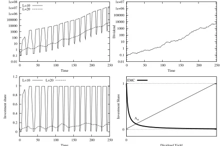
Figure 3: Dynamics with a single mean-variance maximizer in a market with rf = 0.01 and
stochastic dividend with average growth rate g = 0.04 and variance σ2
g = 0.1. Two levels of
memory span of the agent with lower risk aversion are compared. Top-left panel: log-price.
Bottom-left panel: investment shares. Top-right panel: dividend process. Bottom-right panel: equilibrium on the EMC.
To derive all possible equilibria we turn to the deterministic skeleton, fixing σ2
g = 0, let
the price return k∗ be equal to g, and consider the cross-section of investment function (4.2) by the hyperplane (3.10). All the steady-state equilibria can be found as the intersections of the EMC with the cross-section function
˜
fα(y) = min
6
0.99,max
6
0.01,y+g−rf
α
77
, (4.3)
which is shown by the thin curve on the bottom-right panel of Fig. 3. Notice that (4.3) does not depend onL, that is the memory span does not influence the location of the steady-states. Geometrically, all the multi-dimensional investment functions differed only inLcollapse to the same one-dimensional curve. With a single investor the following result follows immediately from Proposition 3.2.
Corollary 4.1. Consider the system (3.2) with g > rf and with a single agent investing
according to (4.2). There exists a unique steady-state equilibrium (x∗, k∗, y∗) and it is charac-terized by k∗ =g and Aα = (y∗, x∗) with:
y∗ =
8
α(g−rf)−(g−rf), x∗ =
9
g−rf
The bottom-right panel of Fig. 3 illustrates this result. The market has a unique steady-state, Aα, whose abscissa, y∗, is the dividend yield, and whose ordinate, x∗, is the agent’s investment share. The position of this steady-state depends on the (normalized) risk aversion coefficient α. It is immediate to see that when α increases, the line x = (y+ g − rf)/α
rotates clockwise, so that the steady-state dividend yield increases, while the investment share decreases. Eq. (4.4) confirms it, as ∂y∗/∂α>0 and ∂x∗/∂α<0.
What are the determinants of stability of the steady-state equilibrium Aα? First of all, notice that we can apply the stability analysis of Section 3.2.3, because the investment function
fα,L is of the type specified in (3.13). The stability, therefore, is determined both by the
memory span L and by the ratio of the slopes of the function ˜fα and the EMC in the point
Aα. Straight-forward computations show that this ratio does not depend onα and it is always equal to −1. Corollary 3.3 then implies that for any given normalized risk aversion α the dynamics stabilizes with high enough memory span L.
To confirm that these results are applicable also for a stochastic system, we simulate the model with investment function ˜fα and stochastic dividend process. We plot the resulting dynamics in Fig. 3. The top-right panel shows the realization of dividend process. Given this process, simulations are performed for investment strategies with the same level of the risk aversion and two different memory spans, collapsed in the same curve as shown in the bottom-right panel. The left panels shows dynamics of prices (top) and investment shares (bottom). When the agents’ memory span L = 10 (solid line), the steady-state is unstable and price fluctuates. These endogenous fluctuations are determined by the upper and lower bounds of the investment function and are much more pronounced than the fluctuations of the exogenous dividend process. When the memory span is increased to L= 20 (dotted line), the system converges to the stable steady-state equilibrium and observed fluctuations are only due to exogenous noise affecting the dividend growth rate.
We turn now to the analysis of a market with many agents, being particularly interested in assessing agents’ survival in the long run. The bottom-right panel of Fig. 4 shows investment functions (4.3) for two different values of risk aversion,αandα$ <α. According to Proposition
3.3, the survivor should have the highest investment share at the steady state. Since at y∗
α the agent with high risk aversion, α, invests less than the agents with low risk aversion,α$, he cannot dominate the market. As a result the steady-state Aα is unstable. Whether the less risk averse agent can dominate the market depends on the stability of the second steady-state,
Aα!, that is on his memory span. If the memory span is high enough, the steady-state Aα! is
stable and the less risk averse agent dominates the market.
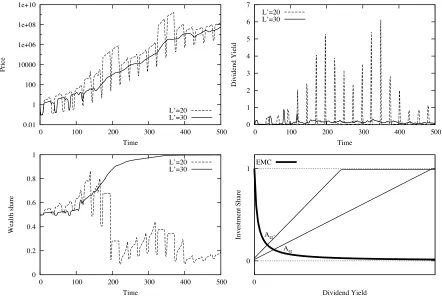
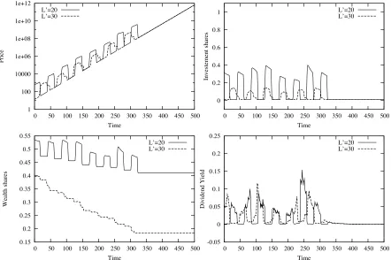
Fig. 4 shows the market dynamics when one agent has risk aversionαand memoryL= 20 (which produces a stable dynamics in a single agent case, cf. Fig. 3), and the other agent has risk aversionα$ <α and memoryL$. Simulations for two different values of the memory span L$ are compared. When the memory span of the less risk averse agent is low, L$ = 20, the
steady-state Aα! is unstable (see dotted lines). Wealth share of both agents keep fluctuating
between zero and one. However, when the memory of the less risk averse agent increases to
L$ = 30, the new steady-state A
α! is stabilized and he ultimately dominates the market (solid
lines). The steady-state return now converges, on average, tog+y∗α! < g+yα∗. Interestingly, in
0.01 1 100 10000 1e+06 1e+08 1e+10
0 100 200 300 400 500
Price
Time
L’=20 L’=30
0 1 2 3 4 5 6 7
0 100 200 300 400 500
Dividend Yield
Time L’=20
L’=30
0 0.2 0.4 0.6 0.8 1
0 100 200 300 400 500
Wealth share
Time
L’=20 L’=30
Investment Share
Dividend Yield A!
A!’
EMC
0 1
[image:19.595.69.511.83.382.2]0
Figure 4: Dynamics with two mean-variance maximizers in a market with rf = 0.01 and
stochastic dividend with average growth rate g = 0.04 and variance σ2
g = 0.1. Two levels of
memory span of the agent with lower risk aversion are compared. Top-left panel: log-price.
Bottom-left panel: wealth share of the agent with lower risk aversion. Top-right panel:
dividend yield. Bottom-right panel: EMC and two investment functions. The agent with lower risk aversion α$ produces the steady state A
α!.
4.2
The LLS model revisited
The insights developed so far can be used to evaluate various simulations of the LLS model performed in Levy, Levy, and Solomon (1994); Levy and Levy (1996); Levy, Levy, and Solomon (2000); Zschischang and Lux (2001). In fact, as far as the co-evolution of prices and wealth is concerned, the LLS model is built on the same framework as considered in this paper.
In the LLS model, agents at period t maximize a power utility function U(Wt+1,γ) = Wt1−+1γ/(1−γ) with relative risk aversionγ >0. Furthermore, to forecast the next period total
return zt+1 =kt+1 +yt+1, agents assume that any of the last L returns can occur with equal
probability. Solutions of the maximization of a power utility are not available analytically but can be shown to give a wealth independent investment shares. This property holds for any perceived distribution, g(z), of the next period total return, which is discrete uniform in this case. Let us denote the expected value of the total return as ¯z, and the corresponding investment function as fEP"γ, g(z)#. As this investment function is unavailable in explicit
form, the analysis of the LLS model relies on numeric solutions.
to invade the market, whereas the memory span influences the stability of the dynamics. These properties hold as long as the investment function on the “EMC plot” shifts upward with decrease of the risk aversion. As the following result shows (see Anufriev, 2008 for a proof), the function fEP"γ, g(z)# has this property.
Proposition 4.1. Let fEP
γ stand for the partial derivative of the investment function fEP
with respect to the risk aversion coefficient γ. Then the following result holds:
If z¯!0, then fEP !0 and fγEP "0 .
In our setting, when a positive return is expected, agents with lower risk aversion invest higher share. Consequently, Propositions 3.3 and 3.4 provide rigorous analytic support to the simulation results of the LLS model.
In Levy and Levy (1996) the focus is on the role of the memory. The authors show that with a small memory span the log-price dynamics is characterized by crashes and booms. Our analysis shows that this result is due to the presence of an unstable steady-state and to the upper and lower bounds of the investment shares. Furthermore, this steady-state becomes stable if the memory is high enough. Simulations in Levy and Levy (1996) confirm this statement; when agents with higher memory are introduced, booms and crashes disappear and price fluctuations become erratic. In our view, these fluctuations around the steady-state of the deterministic system are simply due to the exogenous noise of the dividend process, and not due to the endogenous agents’ interactions.
In Zschischang and Lux (2001) the focus is on the interplay between the length of the memory span and the risk aversion. Their simulations suggest that the risk aversion is more important than the memory span in the determination of the dominating agents, providing that the memory is not too short. The argument has not been put forward in a decisive way though, as the following quote from Zschischang and Lux (2001) (p. 568, 569) shows:
“Looking more systematically at the interplay of risk aversion and memory span, it seems to us that the former is the more relevant factor, as with different [risk aversion coefficients] we frequently found a reversal in the dominance pattern: groups which were fading away before became dominant when we reduced their degree of risk aversion. [...] It also appears that when adding different degrees of risk aversion, the differences of time horizons are not decisive any more, provided the time horizon is not too short.”
Our analytic results make clear how and why this is the case. Agents with low risk aversion are indeed able to destabilize the market populated by agents with high risk aversion. However, this “invasion” leads to an ultimate domination only if the invading agents have sufficiently long memory. Otherwise, and this complements the conclusions of Zschischang and Lux (2001) and related works, agents with different risk aversion coefficients will coexist.
Another new result concerns the case of agents investing a constant fraction of wealth. In Zschischang and Lux (2001) the authors claim that such agents always dominate the market and add (p. 571):
Our analysis allows to make this statement more precise. The agents with constant investment fraction are characterized by the horizontal investment functions, for which Proposition 3.4 guarantees stability, independently of L. If these agents are able to invade the market suc-cessfully, they will ultimately dominate. However, their market invasion will fail, as soon as other agents are more aggressive in the steady-states created by invaders.
5
Non-selecting market dynamics
Our analysis so far dealt with a market where dividends are growing at a higher rate than the risk free asset. Indeed, the steady-state equilibria described in Proposition 3.2 can exist only for g > rf. One may wonder what happens in the opposite case, when the dividends
grow, on average, more slowly thanrf. For instance, some simulations of the LLS model were
performed with positive risk-free rate and constant dividend (i.e.g = 0), and these simulations do converge. To understand why and where they converge in this Section we return to the setting with general investment functions and analyze the case of g < rf. We show that
prices are always growing at the rate rf, no matter the initial set of investment strategies.
Furthermore, the dividend yield converges to y∗ = 0. As a result the wealth return is rf for
any investment strategy, and no selection on the set of investment strategies occurs.
The reason why we did not find any steady-state when g < rf despite a convergence of
the LLS simulations is very simple. Since the domain D given in (3.5) is not a closed set, the dynamics can easily converge to a point which is outside of D. One possibility is the point with zero dividend yield, another is where the price return k∗ = −1. Both cases were not included in the definition of domain D, because they lie outside the possibilities considered in our model. In the former case the dividend must be zero, while in the latter case the price sequence is not defined.
Formally, however, the dynamics (3.2) is well defined also on the set
D$ = (0,1)N ×∆N ×[−1,∞)L×[0,∞)L. (5.1)
Let us, therefore, extend our analysis on the dynamics defined on D$, and in this way char-acterize possible behaviors of the system when it is asymptotical converge to a steady-state equilibrium with zero dividend yield. The next result applies.
Proposition 5.1. Consider the dynamical system (3.2) evolving on the set D$ introduced in (5.1) and assume that the no-short selling constraint (3.3) is satisfied. Apart from the steady-state equilibria described in Proposition 3.2, the system has other steady-states equilibria
(x∗1, . . . , x∗N;ϕ∗1, . . . ,ϕ∗N;k∗;y∗) where:
- The price return is equal to the risk free rate, k∗ =r f.
- The dividend yield is zero, y∗ = 0.
- The wealth shares satisfy
1
ϕ∗m ∈(0,1] if m≤M
ϕ∗m = 0 if m > M
and
N
!
m=1
ϕ∗m = 1. (5.2)
0.01 1 100 10000 1e+06 1e+08 1e+10
0 100 200 300 400 500
Price
Time L=10
L=20
0.01 1 100 10000 1e+06 1e+08
0 100 200 300 400 500
Dividends
Time
0 0.2 0.4 0.6 0.8 1
0 100 200 300 400 500
Investement shares
Time
L=10 L=20
0 0.05 0.1 0.15 0.2 0.25
0 100 200 300 400 500
Dividend Yield
Time
[image:22.595.69.512.85.380.2]L=10 L=20
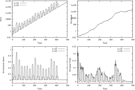
Figure 5: Dynamics with a single mean-variance maximizer in a market with rf = 0.05 and
stochastic dividend with average growth rateg = 0.04 and varianceσ2
g = 0.1. Top-left panel:
log-price for two different values of memory spanL. Bottom-left panel: investment shares.
Top-right panel: dividend process. Bottom-right panel: dividend yield.
Contrary to the steady-state equilibria with positive dividend yield, in the steady-states derived in Proposition 5.1, the total return of the asset, k∗+y∗, coincides withrf, the return
of the risk-less asset. In these steady-states, therefore, there is no difference in the investment opportunities. The investment shares of agents are unambiguously determined through the investment functions, while the wealth shares are free of choice, so that any number of agents can survive. Survivors may behave differently, i.e. homogeneous behavior is not necessary, as opposed to the steady-states with positive yield. This is due to the fact that the total return is the same for all investment strategies.
Corollary 5.1. At any steady-state equilibrium with y∗ = 0 as found in Proposition 5.1, the wealth return of each agent is equal to rf.
The local stability of the steady-state equilibria with zero dividend yield can be analyzed along the same lines of Proposition 3.3.
Proposition 5.2. Steady states of the dynamical system (3.2) evolving on the set D$, in
which the dividend yield is zero, can be stable only if the dividend growth rate g is less than
the risk-free interest rate rf.
Let g < rf and let
"
x∗
1, . . . , x∗N;ϕ∗1, . . . ,ϕ∗N;k∗;y∗
#
be a fixed point of (3.2) with y∗ = 0.
This point is locally stable if all the roots of polynomial
Q0(µ) =µL+1+ - 1 +rf
x∗(1−x∗).(1−µ)
!L−1 l=0
1 100 10000 1e+06 1e+08 1e+10 1e+12
0 50 100 150 200 250 300 350 400 450 500
Price
Time L’=20
L’=30
0 0.2 0.4 0.6 0.8 1
0 50 100 150 200 250 300 350 400 450 500
Investement shares
Time
L’=20 L’=30
0.15 0.2 0.25 0.3 0.35 0.4 0.45 0.5 0.55
0 50 100 150 200 250 300 350 400 450 500
Wealth shares
Time
L’=20 L’=30
-0.05 0 0.05 0.1 0.15 0.2 0.25
0 50 100 150 200 250 300 350 400 450 500
Dividend Yield
Time
[image:23.595.70.512.84.378.2]L’=20 L’=30
Figure 6: Dynamics with two mean-variance maximizers in a market with rf = 0.05 and
stochastic dividend with average growth rate g = 0.04 and variance σ2
g = 0.1. Two levels
of memory span of the agent with lower risk aversion are compared. Top-left panel: log-price dynamics. Bottom-left panel: wealth share of the agent with lower risk aversion α$. Top-right panel: investment shares. Bottom-right panel: dividend yield.
lie inside the unit circle.
The steady-state is unstable if at least one of the roots of polynomial Q0(µ) is outside the unit circle.
Proof. See Appendix G.
As a comparison with results from the previous section, in Figs. 5 and 6 we plot the results of market simulations when agents are mean-variance optimizers, with investment functions (4.2). Fig. 5 shows market dynamics for a single agent with memory span either L = 10 or
L= 20. The only difference between simulations shown in Fig. 5 and those in Fig. 3 is the risk free rate, which is now equal to 0.05, so thatg < rf. Whereas withg > rf the market is stable
with long memory and unstable with high memory, withg < rf the market dynamics stabilizes
no matter the value ofL.11 Moreover, the price grows at the constant rater
f (top-left panel),
no matter the exogenous fluctuations of the dividend process (top-right panel). Since the price grows faster than the dividend, the dividend yield converges to 0 (bottom-right panel). Notice also that at the steady-state the agent is investing a constant fraction of wealth equal to the lower bound of (4.2), i.e. x∗ = 0.01 in this case (bottom-left panel).
11By applying Proposition 5.2 to the investment function f in (4.2), and noticing that, due to the lower
bound, the investment function is always flat aty∗= 0, it can be shown that the steady-statey∗= 0 is stable