Non parametric methods applied in the efficiency analysis of European structural funding in Romania

Non-parametric methods applied in the

efficiency analysis of European structural

funding in Romania

Roman, Monica and Gotiu (Lucaciu), Liliana

Bucharest University of Economic Studies, Bucharest University of

Economic Studies

17 March 2017

Online at

https://mpra.ub.uni-muenchen.de/80548/

Non-parametric methods applied in the efficiency analysis of

European structural funding in Romania

Authors:

Monica Roman, Bucharest University of Economic Studies

Liliana Lucaciu (Gotiu), Bucharest University of Economic Studies

Abstract

One of the most widely used methods in assessing the efficiency of public policies and

programs for a set of units is Data Envelopment Analysis (DEA). DEA is a non-parametric

method which identifies an efficiency frontier on which only the efficient Decision Making

Units (DMUs) are placed, by using linear programming techniques. By applying

non-parametric techniques of frontier estimation, the efficiency of a DMU can be measured by

comparing it with an identified efficiency frontier. In this paper we have used DEA for

evaluating the efficiency of the European structural funds allocated to finance the educational

infrastructure through the Regional Operational Program 2007-2013, implemented in

Romania. The output variables measure the educational performance as well as the school

drop-out rate, while the focal input variable is the value of European funds. Romanian

counties are considered to be the decision making units (DMUs). Our results confirm the deep

disparities existing between Romanian counties concerning the efficient use of European

structural funds.

Keywords: European structural funds, efficiency, Data envelopment analysis, infrastructure,

regions

JEL classification: H83, R58, C61

1

1 Introduction

After becoming a Member State of the European Union, starting with the

programming period of 2007-2013, Romania benefited from structural and investment funds2,

designed to help it cope with the economic challenges and disparities, as well as to take

advantage of the opportunities available in the country. For Romania, the European Union

funds represent financial instruments set up to assist in reducing the regional disparities and

fostering growth through investments in domains such as employment, social inclusion, rural

and urban development or research and innovation. During the programming period

2007-2013, Romania benefited from a budget of 27.5 billion euros, out of which 19.2 billion euros

were for the structural and cohesion funds and 8.3 billion for the Common Agricultural

Policy.

The aim of the paper is to analyse the regional disparities existing between Romanian

counties regarding the efficiency of the European structural funds3 (hereafter SF) allotted for

financing the educational infrastructure. One of the most relevant needs for Romania’s social

development is improving the quality of educational infrastructures and reducing the regional

disparities existing between Romanian regions in this case. The Regional Operational

Programme through the Key Area of Intervention 3.4 „Rehabilitation, modernisation,

development and equipping of pre–university, university education and continuous vocational

training infrastructure” was the programme that addressed the needs for the educational

infrastructure development.

2

Since 2007, the EU Cohesion policy has revolved around three objectives: Convergence (81.7% of the total Cohesion Policy payments), Competitiveness and employment (15.8%) and Territorial cooperation.

3

In this research we have used a non-parametric method widely utilised for evaluating

the efficiency of regional units, namely Data Envelopment Analysis (DEA). The efficiency

was computed in various models, both output and input oriented, using STATA 20.

The contribution of the paper is twofold: the paper approaches the efficiency of using

structural funds in the first Programming period in Romania, being one of the first attempts to

apply DEA methodology in this respect; at the same time, the study is focused on the

counties, at NUTS3 level, and ways to improve regional policies implementation in Romania,

in the second programming period, 2014-2020. The study fills a gap in the literature related to

public programming and planning, provides valuable information for decision makers and

also opens room for further research on this challenging topic.

This paper is structured as follows: The second section presents the Romanian context

related to the existing needs in education, while Section 3 briefly reviews the literature on the

impact of structural funds on economic growth and the economic convergence process,

respectively. Sections 4 and 5 discuss the method applied and subsequently the variables and

model specifications, followed by the presentation of the results in Section 6. Finally, section

7 concludes.

2 The Romanian context: needs in the educational system and policy responses

A basic structure of education levels in Romania includes: kindergarten, primary

school, middle school, high school and higher education and education in Romania is

compulsory for 11 years (from the preparatory school year to the tenth grade). With the

exception of kindergarten and higher education, the private sector has a very low presence in

the Romanian education system. Therefore, the education system is mainly financed from the

state budget; the general government expenditure on education as a share of GDP fell from

sector. This is reflected in low wages, but also in the poor state of the educational equipment,

learning spaces, as well as in the related facilities.

The situation is even more difficult for the schools in disadvantaged communities. In a

report published in 2014, Fartușnic et al. found that the core financial source of these schools

is state funding and their entire annual budget covers only administrative costs and teachers’

salaries. It seems obvious that such institutions have insufficient resources for infrastructural

development.

The access to schooling of children from disadvantaged areas, especially from rural

areas, but also of those from vulnerable social environments is difficult in Romania. In some

cases, school capacity is deficient; there are large distances to the closest school and

inadequate transportation facilities. A large number of education units need rehabilitation

works and equipping with didactic equipment, IT and specific documentation materials.

Fartușnic (2014) noticed that according to the data on early school leaving provided by the

Romanian National Institute for Statistics, the share of early school leavers in rural areas is

three times higher than in urban areas and there are also important differences between

Romanian regions: the highest rates were recorded in the North-East, South-East and South

Muntenia regions, while the lowest were in the Bucharest Ilfov and Western regions.

Under such circumstances, the national strategy in the field made it a priority to set up

and develop the education infrastructure, to increase education accessibility and quality. The

Regional Operational Programme 2007 – 2013 through the Key Area of Intervention 3.4.

“Rehabilitation, modernisation, and development and equipping of pre-university, university

education and continuous vocational training infrastructure” (hereafter KAI 3.4) has the

purpose to address the existing needs. In terms of the activity proposals, the activities that

required special attention referred to “the construction, consolidation, rehabilitation,

equipment with teaching materials, professional training materials, IT equipment and specific

equipment for residential spaces; the rehabilitation, consolidation, modernisation of buildings

and fields on university campuses; the rehabilitation and/or consolidation of buildings located

within the continuous professional formation institutions; and the modernisation of utilities,

including the demand for special facilities for people with disabilities, for all types of

infrastructure”4

In the context of a chronic lack of financial resources invested in education in the past 25

years, the successful implementation of the projects financed through European SF at national

level becomes a top priority. The efficiency of using SF is crucial, since the specific needs are

usually in high numbers and of significant relevance and the final goal is increasing the

quality and performance of the education system in Romania. It is important to mention that

this paper does not provide an impact analysis of SF, but an evaluation of the efficiency of

using SF in achieving the specific objectives.

3 Literature review

Given the relevance and the high interest in the EU Cohesion Policy, the evaluation of the

performances of various financing programs has become a high priority and it involved a

large spectrum of both quantitative and qualitative methods. In their paper (2010) Mohl and

Hagen prove that the econometric evaluation of EU Cohesion Policy is hampered by several

econometric issues, such as reverse causality, measurement error, omitted variables, strict

functional form assumptions and the potential inclusion of inappropriate control variables.

Starting with this finding, we attempted to apply non-parametric methods for evaluating the

performance in using structural funding at regional level in Romania. The existing results on

4

the efficiency of using structural funds for the regional development are relying mainly on

parametric approaches and econometric modelling. The advantages of non-parametric

approaches are less exploited and this paper aims at testing the performance of such

techniques in this field.

DEA approach involves the application of the linear programming technique to trace the

efficiency frontier. It was originally developed to measure the performance of various

non-profit organizations, such as educational and medical institutions, which were highly resistant

to traditional performance measurement techniques due to the complex and often unknown

relations of multiple inputs and outputs and non-comparable factors that had to be taken into

account. In recent years it has been successfully applied in measuring the efficiency of both

for-profit and non-profit organizations, such as the effectiveness of regional development

policies in Northern Greece by Karkazis and Thanassoulis (1998). Coelli, Rao and Battese

(1998) introduce the reader to this literature and describe several applications. DEA was

launched by Charnes et al. (1978) under the assumption that production exhibited constant

returns to scale. Banker et al. extended it to the case where there are variable returns to scale.

Governmental efficiency in general and public policies efficiency became research

subjects of an increasing number of papers. Zhu (2002) provides a series of Data

Envelopment Analysis (DEA) models for efficiency assessment and for decision making

purposes. Rhodes and Southwick (1986) use DEA to analyze and compare private and public

universities in the USA. More recently, Singh (2016) uses DEA for ranking the Indian states

in their efficiency of applying a large welfare scheme for poverty alleviation. Using a sample

of 31, an input and output oriented DEA model was applied, with constant and variable return

to scale proving that 11 units were technically efficient.

There are several applications of the DEA method for Romania; Roman and Suciu (2012)

Nitoi (2008) assesses the efficiency of the Romanian banking system using an input oriented

with variable returns to scale DEA model. DEA has also been used to assess different aspects

of the medical field like hospital efficiency (Nedelea et al., 2010; Mecineanu et al., 2012) or

health systems efficiency (Asandului, Roman, Fatulescu, 2014).

USING a panel of NUTS3 regions, Becker et all (2010) find positive growth effects of

Objective 1 funds, but no employment effects. Puigcerver-Peñalver (2007) finds that

structural funds have positively influenced the growth process at regional level although their

impact has been much stronger during the first Programming period than during the second

one. Rodriguez-Pose and Fratesi (2004) distinguish between various structural funds

expenditure and conclude that only structural fund expenditures for education and investment

have a positive effect in the medium run, whereas expenditures for agriculture do not.

Mohl and Hagen (2010) evaluate the growth effects of European structural funds

payments at regional level. Using a new panel dataset of 124 NUTS regions for the time

period 1995-2005, they found empirical evidence that the effectiveness of structural funds in

promoting growth is strongly dependent on which financing objective is analysed. The

payments of Objective 2 and 3 have a negative effect on GDP.

4 Method and models specifications

First presented in 1978 and based on the paper of Farrell, the first DEA model is

known in the literature as the CCR model, after its authors, Charnes, Cooper and Rhodes. It is

a non-parametric method which identifies an efficiency frontier on which only the efficient

Decision Making Units (DMUs) are placed, by using linear programming techniques. The

method depends on a number of output and input variables that are employed for computing

Since it is of high importance which are the variables selected in the model and how

many these are, a strong experience in the field of application of the method is needed. At the

same time, the number of DMU could also be a challenge for applying the method in public

policy evaluation: for the purpose of the paper, we follow the suggestion of Mohl and Hagen

(2010) who recommend to use regional data that would allow for a more accurate analysis of

the funding’s efficiency and also for maximizing the discrimination existing between various

DMU.

In general there is a trade-off between the number of variables included in the models

and the number of DMU and this issue was studied by various researchers. For instance,

Dyson et al. (1991) recommend a total of two times the product of the number of inputs and

outputs variables. Golany and Roll (1989) recommended that the number of DMU should be

at least twice the number of inputs and outputs considered. On the other hand, Charnes and

Cooper (1991) have suggested that there should be three times as many DMUs as the number

of inputs plus outputs.

Following the rule of thumb suggested by Cooper et al (2007) we estimate that the

minimum number of DMUs required is achieved:

n ≥ max{m * s, 3(m + s)} ,

where n is the number of DMUs, m is the number of inputs and s is the number of outputs. For a model relying on three inputs and three outputs, as in the present research, it would be

recommended that at least 18 DMUs should be included in the estimation of the efficiency

frontier. This condition is satisfied, since there are 31 DMUs involved in the analyzed models.

4.1 Model for an output-oriented specification

The DEA models could be input or output oriented: an input-orientated model looks at the

output-oriented DEA model looks at maximizing the outputs obtained by the DMUs while keeping

the inputs constant.

In the particular case of our research, the linear programming problem to be solved, in the

output oriented and variable-returns to scale hypothesis, is sketched below (Charnes, Cooper

and Rhodes, 1978).

Suppose there are k inputs and m outputs for n DMUs. For the i-th DMU, yi is the column

vector of the inputs and xi is the column vector of the outputs. We can also define X as the

(k×n) input matrix and Y as the (m×n) output matrix. The DEA model is then specified with

the following mathematical programming problem, for a given i-th DMU:

                 0 1 0 0 1 ,

max

In problem (1),  is a scalar and 1.

-1 is the proportional increase in outputs that could be achieved by the i-th DMU with the

input quantities held constant.

The measure 1/ is the technical efficiency score and varies between 0 and 1. If it is less than

1, the public intervention is inside the frontier (i.e. it is inefficient), while if it is equal to 1 it implies that the intervention is on the frontier (i.e. it is efficient).

The λ vector is a (n×1) vector of constants that measures the weights used to compute the location of an inefficient DMU if it were to become efficient. The inefficient DMU would be

peers of the inefficient DMU. The peers are other DMUs that are more efficient and therefore

are used as references for the inefficient DMU. N1 is a n-dimensional vector of ones.

Adding the restriction

N1 λ< = 1 in DEA model

the convexity of the frontier is imposed, accounting for variable returns to scale. Dropping

this restriction would amount to admit that returns to scale were constant. The linear

programming problem (1) is solved for each of the n DMUs resulting in n efficiency scores. The scale efficiency could also be computed for the DMUs in the sample. This is the ratio

between the efficiency scores in the CRS and VRS hypotheses and accounts for the increase,

decrease or constant return to scale.

4.2 Model for an input-oriented specification

The specifications of the mathematical programming problem, for a given i-th DMU are

described below, and one problem for each DMU has to be solved:

                0 1 N 0 X x 0 Y y min 1 i i ,         (2)

In the problem above, the inverse of scalar θ ranges between 0 and 1 and is the technical

efficiency score. Like in the previous case, if it is equal to 1, it implies that the DMU is

efficient, while if it is less than 1, the DMU is inefficient. The model specification under the

hypothesis of variable return to scale implies the condition of convexity of the frontier.

In the present research we have applied the DEA input and output oriented models

considering both the constant and variable return to scale and the scale efficiency was also

5 Model specifications and data

The variable of interest in our models is the total value of the projects financing the

educational infrastructure through KAI 4.3 at county level. Out of the total number of projects

contracted, we have selected the projects which had been finalized by April 2014, resulting

131 projects with a total value of 723 million lei. The projects devoted to financing higher

education and research infrastructure were in a small number and therefore were excluded

from the analysis. The data is provided by the Ministry of Regional Development and Public

Administration and it covers the projects financed between 2007 and 2014. Other two inputs

also considered in the efficiency evaluation are: the teacher/student ratio that counts for the

human resources and the number of classrooms/student ratio that counts for fixed capital. The

data provided by the National Institute for Statistics refers to 2014.

The output variables were selected in line with one of the objectives of the KAI 3.4,

that were to increase the educational performance and accessibility. Therefore, the average

pass rates at the National Evaluation and the National Baccalaureate exam were included in

the set of output variables, as proxy for educational performance. These indicators are

reported by the Ministry of National Education at various regional levels, counties included.

The variation of dropout rate was included as the third output, as a measure of the education

accessibility. The variable is reported at county level by National Institute of Statistics. The

output variables refer to 2014 (dropout rate) and 2015 (graduation rates), knowing that it takes

a period of time for a programme to produce effects. As in other studies (Roman and Suciu,

6 Results and discussions

6.1 Data and variables

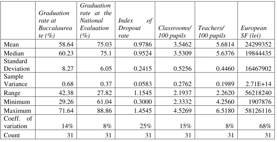
Table 1 summarizes the descriptive statistics for the set of input and output variables.

The two indicators accounting for the performance of the undegraduate education system,

namely the graduation rate at the Baccalaureate exam and the graduation rate at the National

Evaluation, provide a moderate homogeneity. The first one has the minimum value recorded

in Ilfov (29,26%), that is an outlier of the series, while the maximum graduation rate was

registered in Cluj (71,74%). The mean of the sample is 58,64%, in line with the national

average of 59,25%. The graduation rate for the National Evaluation ranges from a minimum

score of 61,04% in Olt to 88% in Cluj, with an average of 75%.

Table 1. Descriptive statistics of the selected variables

Graduation rate at Baccalaurea te (%)

Graduation rate at the National Evaluation (%)

Index of

Dropout rate

Classrooms/ 100 pupils

Teachers/ 100 pupils

European SF (lei)

Mean 58.64 75.03 0.9786 3.5462 5.6814 24299352

Median 60.23 75.1 0.9524 3.5309 5.6376 19844435

Standard

Deviation 8.27 6.05 0.2415 0.5256 0.4460 16467902

Sample

Variance 0.68 0.37 0.0583 0.2762 0.1989 2.71E+14

Range 42.38 27.82 1.1545 2.1937 2.2620 56218240

Minimum 29.26 61.04 0.3000 2.3332 4.2560 1907876

Maximum 71.64 88.86 1.4545 4.5269 6.5180 58126116

Coeff. of

variation 14% 8% 25% 15% 8% 68%

Count 31 31 31 31 31 31

The modest performance of the undegraduate education system generated vivid

debates in the Romanian media and also among education decision makers and researchers

that tried to identify the possible causes for the situation, spreading from the poor education

parental involvement, to the shifts in youth behavior and lack of student interest in learning

and preparing for a career.

The variation of the dropout rate has a moderate homogeneity described by a

coefficient of variation of 25% and the mean and median are very close to each other,

pointing out the symmetry of the series. On average, the counties in the sample faced a slow

decrease in the dropout rate, but, at the same time, there are regional differences. The highest

decrease in the dropout rate (by 70%) appears in Hunedoara, while the highest increase (of

38%) is registered in Ilfov. Variables accounting for human and fixed capital are homogenous

and Ilfov is again in the most disadvantageous situation with the minimum values of 2.3

classrooms per 100 pupils and 4.2 teachers per 100 students. The best ranked are Sălaj and

Vâlcea. The values of ESF are by far the most heterogeneous, having a coefficient of variation

of 68%. Maramureş attracted the lowest amount, while Dâmboviţa attracted the highest

amount. The distribution of the European funds across Romanian counties, also presented in

Figure 1, confirms the important differences in attracting European funds for the educational

infrastructure. Although all of the Romanian counties seem to have similar problems related

to the lack of finance for education, many of these were not successful in applying for or

implementing projects for tackling this issue.

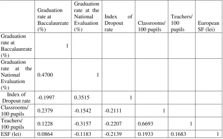
The correlation matrix was computed as a decision instrument in selecting the input and

output variables. If there are strong correlations between these variables, the number of

variables could be reduced by eliminating some of the variables correlated. The values of the

correlation coefficients reported below show that all the variables considered for the analysis

could be included in the DEA models, since the correlation existing between them is modest.

It should be noted that the statistical significance of the Pearson’s correlation coefficients

reported in Table 2 is not of interest for this research, as the statistical inference is not

Figure 1.

Source: authors’ computations, based on data from Ministry for Regional Development and Public Administration, www.inforegio.ro

In order to reduce the heterogeneity in the dataset, the log transformation was applied on the

data. The newly created variable has a coefficient of variation of 5%.

Table 2. Correlation matrix for the input and output variables

Graduation rate at Baccalaureate (%) Graduation rate at the National Evaluation (%)

Index of Dropout rate Classrooms/ 100 pupils Teachers/ 100 pupils European SF (lei) Graduation rate at Baccalaureate (%) 1 Graduation rate at the National Evaluation (%)

0.4700 1

Index of

Dropout rate -0.1997 0.3515 1

Classrooms/

100 pupils 0.2379 -0.1542 -0.2111 1

Teachers/

100 pupils 0.1228 -0.3157 -0.2207 0.6693 1

ESF (lei) 0.0864 -0.1183 -0.2139 0.1933 0.1683 1

0 10000000 20000000 30000000 40000000 50000000 60000000 70000000 MA R A MU R E S S U CE A V A IL F O V T UL CE A V A S L UI MU R S V A L CE A BUZA U S IB IU V R A N CE A DO L J CO V A S N A BA CA U CO N S T A N T A CA R A S S A T U MA R E BI H O R BR A S O V CL UJ BI S T R IT A O L T IA S I G A L A T I S A L A J BR A IL A A R G E S H A R G H IT A N E A M T H UN E DO A R A A R A D DA MB O V IT A

6.2 Results of the DEA analysis

Several DEA models, both input and output oriented were applied for better evaluating

the efficiency of European SF invested in education in Romania.

In the first DEA input oriented Model 1.1, we consider the European SF as input variable and the three output variables. There are eight counties on the efficiency frontier,

namely: Brăila, Cluj, Harghita, Ilfov, Maramureş, Suceava, Vaslui and Vrancea (see Table A1

in the Appendix). These counties were less successful in attracting SF, and yet they manage

to generate good education performance. This implies that SF only are not a sufficient

condition for achieving educational performance, and they need to be supported with other

resources. Model 1.2 described below includes all the input and output variables for

generating TE scores, computed in the CRS and VRS versions of DEA.

The average efficiency score under the assumption of constant return to scale is 0.887,

while in the case of variable return to scale the average efficiency is slightly higher, 0.919. In

both cases, the scores distributions are homogeneous. In practice, it is less likely to have

constant return to scale, and therefore in the following table the results from Model 1.2, input

oriented with VRS, are detailed.

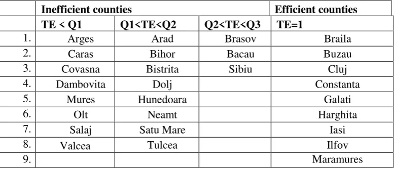
Table 3. Results from the Model 1.2, input oriented with VRS: counties distributed

according to efficiency scores.

Inefficient counties Efficient counties

TE < Q1 Q1<TE<Q2 Q2<TE<Q3 TE=1

1. Arges Arad Brasov Braila

2. Caras Bihor Bacau Buzau

3. Covasna Bistrita Sibiu Cluj

4. Dambovita Dolj Constanta

5. Mures Hunedoara Galati

6. Olt Neamt Harghita

7. Salaj Satu Mare Iasi

8. _Valcea Tulcea Ilfov

10. Suceava

11. Vaslui

12. Vrancea

The median score is 0.932, slightly higher compared to the average, implying a

dominance of high values which is also reflected by the share of counties situated on the

efficiency frontier.

We consider that the most appropriate model for the current research is the output

oriented one, which assumes maximizing the outputs with the same level of inputs. Keeping

in mind that the expected impact of investing SF in educational infrastructure is improving the

educational performance of students, by increasing the quality of the educational facilities, the

focus of the output oriented model is on the output indicators: the model assumes the

maximization of output variables, achieved with given inputs. Therefore, the most relevant

models seem to be the DEA output oriented models, described in the following part of the

paper. The efficiency scores for the applied DEA models are reported in Appendix.

The first output oriented DEA model considers the SF as input variable and the three

output variables. On the efficiency frontier we find almost the same counties as in the input

oriented specification model: Brăila, Cluj, Hunedoara, Iasi, Maramures, Suceava, Tulcea and

Vâlcea (see Table A2 in Appendix). With the exception of Hunedoara County, all the other

counties have registered low levels of SF invested in educational infrastructure, implying that

high levels in the output variables were achieved with fixed, yet low levels SF.

Under these circumstances it is interesting to analyze the counties’ performance when

the set on input variables is increased with human resources and fixed capital. The average

efficiency scores are 0.885 in the CRS version and 0.928 under the VRS assumption. The

extended results after applying the DEA model in the complete model specification,

scores were computed in both the CRS and VRS versions of DEA, in the following table we

report the synthesis of the results of the VRS model.

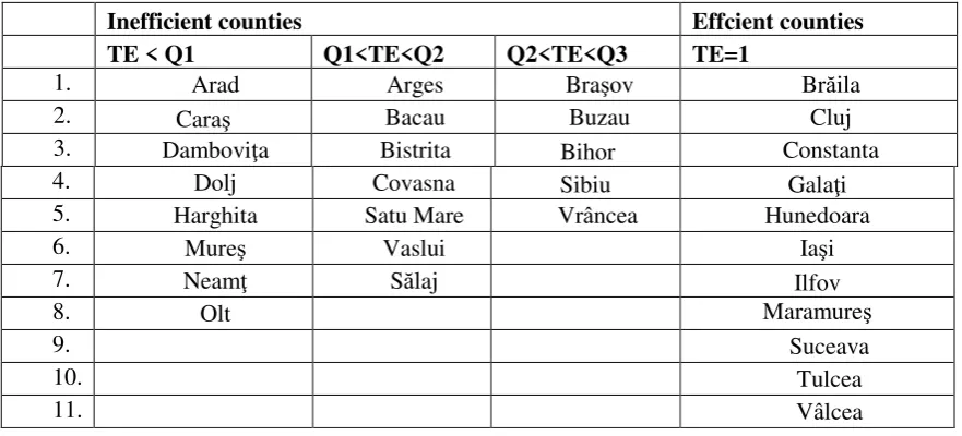
Table 4. Results of Model 2.2, output oriented with VRS: counties distributed according

to efficiency scores.

Inefficient counties Effcient counties

TE < Q1 Q1<TE<Q2 Q2<TE<Q3 TE=1

1. Arad Arges Braşov Brăila

2. _Caraş Bacau Buzau Cluj

3. Damboviţa Bistrita Bihor Constanta

4. Dolj Covasna Sibiu Galaţi

5. Harghita Satu Mare Vrâncea Hunedoara

6. Mureş Vaslui Iaşi

7. Neamţ Sălaj Ilfov

8. Olt Maramureş

9. Suceava

10. Tulcea

11. Vâlcea

The results in Table 4 deserve further discussion. The distribution of the counties

seems to be more balanced compared to Model 1.2 and the median score is 0.924, almost

identical with the mean value. In the first quartile there are eight counties that are the least

efficient. These counties have modest education performance, but manage to attract high

amounts of funding for improving their educational infrastructure. Counties such as Arad,

Dâmboviţa or Harghita are among the top recipients of such financial resources, but the

efficiency of using them is relatively low. In the second group, with efficiency scores

ranging between the first and second quartile, there are seven counties, while five counties

have efficiency scores between the second and third quartile. Among these are counties

such as Braşov, Vrâncea, Sibiu, Bihor or Buzau. About one third of the counties in our

sample are efficient: Brăila, Cluj, Constanţa, Galaţi, Hunedoara, Iaşi, Ilfov, Maramureş and

counties like in the previous models. Among these we found counties that have attracted

financial resources above the average and managed to report good educational

performance. These counties are Brăila, Galaţi, Hunedoara and Iaşi. On the efficiency

frontier there are also counties with the lowest values of attracted funds and with low

levels of output indicators, such as Maramureş, Vâlcea, Tulcea, Ilfov. These results

confirm that when combined with human resources and fixed capital, the SF invested

through KAI 4.3 in Romania has led to higher values of output indicators.

The scale efficiency was also considered in the analysis, and scale was computed as

the ratio between efficiency scores produced in the CRS and VRS models. Not

surprisingly, the findings from both CRS and VRS models reflect a decreasing return to

scale for the great majority of the DMUs, with a coefficient of returns to scale lower than

1. This implies that an increase in inputs will generate a smaller increase in outputs.

Finally, five counties that were efficient in both models presented are also scale efficient:

Brăila, Constanţa, Galaţi, Ilfov, Maramureş, and Suceava.

7 Conclusions

In this research, the efficiency in using European structural funds for improving the

educational infrastructure was computed in several DEA models, both output and input

oriented. More than that, in the developed models both CRS and VRS was employed, the

focus being on output oriented model with VRS. The results confirm that there are disparities

among Romanian counties: the counties with a low accession rate to structural funds are the

ones with the lowest efficiency scores: Caraş, Vălcea, Mureş, Dâmboviţa, Sălaj, Olt. On the

other hand, on the efficiency frontier we have found counties with high SF values: Brăila,

The conclusions confirm the efficiency in using European structural funds in a number

of counties that have attracted important amounts of money, but at the same time there are

counties which are far from the efficiency frontier.

It is important to mention that our purpose in not to assess the impacts of the KAI 3.4

and the current research does not have the ambition of providing an impact evaluation, but to

assess the efficiency of using European SF, at county and regional level and to provide a

ranking of Romanian counties. This can be a strong starting point in validating the future

impact evaluations of the programme and also in understanding the regional disparities in

accessing SF for education. The projects implemented in counties with modest technical

efficiency scores could be closer monitored and better supported in achieving their results. In

such cases, the county administration needs to support various projects for generating a

synergetic effect that could contribute to decreasing the regional disparities existing in the

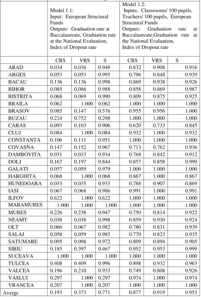
Appendix: Efficiency scores from DEA models Table A1

Input oriented models

Model 1.1:

Input: European Structural Funds

Outputs: Graduation rate at Baccalaureate, Graduation rate at the National Evaluation, Index of Dropout rate

Model 1.2:

Inputs: Classrooms/ 100 pupils, Teachers/ 100 pupils, European Structural Funds

Outputs: Graduation rate at Baccalaureate,Graduation rate at the National Evaluation,

Index of Dropout rate

CRS VRS S CRS VRS S

ARAD 0.034 0.036 0.948 0.832 0.908 0.916

ARGES 0.053 0.053 0.995 0.796 0.848 0.939

BACAU 0.136 0.136 0.998 0.869 0.938 0.926

BIHOR 0.085 0.086 0.988 0.858 0.869 0.987

BISTRITA 0.068 0.069 0.990 0.809 0.875 0.925

BRAILA 0.062 1.000 0.062 1.000 1.000 1.000

BRASOV 0.085 0.147 0.576 0.955 0.956 1.000

BUZAU 0.224 0.752 0.298 1.000 1.000 1.000

CARAS 0.093 0.103 0.906 0.620 0.733 0.845

CLUJ 0.084 1.000 0.084 0.932 1.000 0.932

CONSTANTA 0.106 0.111 0.951 1.000 1.000 1.000

COVASNA 0.147 0.152 0.967 0.713 0.762 0.936

DAMBOVITA 0.031 0.033 0.934 0.768 0.842 0.912

DOLJ 0.167 0.197 0.844 0.857 0.858 0.999

GALATI 0.057 0.059 0.979 1.000 1.000 1.000

HARGHITA 0.068 1.000 0.068 0.867 1.000 0.867

HUNEDOARA 0.033 0.035 0.933 0.788 0.907 0.869

IASI 0.067 0.068 0.986 0.991 1.000 0.991

ILFOV 0.622 1.000 0.622 1.000 1.000 1.000

MARAMURES 1.000 1.000 1.000 1.000 1.000 1.000

MURES 0.226 0.238 0.947 0.750 0.814 0.922

NEAMT 0.038 0.038 0.998 0.859 0.930 0.924

OLT 0.066 0.067 0.982 0.780 0.831 0.939

SALAJ 0.058 0.059 0.985 0.770 0.823 0.935

SATUMARE 0.095 0.098 0.972 0.809 0.894 0.905

SIBIU 0.185 0.397 0.467 0.952 0.953 0.999

SUCEAVA 1.000 1.000 1.000 1.000 1.000 1.000

TULCEA 0.408 0.409 0.996 0.898 0.932 0.963

VALCEA 0.196 0.210 0.933 0.749 0.808 0.926

VASLUI 0.297 1.000 0.297 0.974 1.000 0.974

VRANCEA 0.207 1.000 0.207 1.000 1.000 1.000

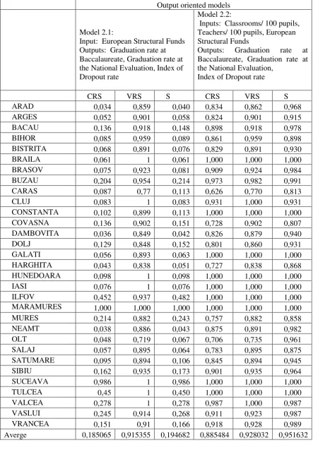
Table A2

Output oriented models

Model 2.1:

Input: European Structural Funds Outputs: Graduation rate at Baccalaureate, Graduation rate at the National Evaluation, Index of Dropout rate

Model 2.2:

Inputs: Classrooms/ 100 pupils, Teachers/ 100 pupils, European Structural Funds

Outputs: Graduation rate at Baccalaureate, Graduation rate at the National Evaluation,

Index of Dropout rate

CRS VRS S CRS VRS S

ARAD 0,034 0,859 0,040 0,834 0,862 0,968

ARGES 0,052 0,901 0,058 0,824 0,901 0,915

BACAU 0,136 0,918 0,148 0,898 0,918 0,978

BIHOR 0,085 0,959 0,089 0,861 0,959 0,898

BISTRITA 0,068 0,891 0,076 0,829 0,891 0,930

BRAILA 0,061 1 0,061 1,000 1,000 1,000

BRASOV 0,075 0,923 0,081 0,909 0,924 0,984

BUZAU 0,204 0,954 0,214 0,973 0,982 0,991

CARAS 0,087 0,77 0,113 0,626 0,770 0,813

CLUJ 0,083 1 0,083 0,931 1,000 0,931

CONSTANTA 0,102 0,899 0,113 1,000 1,000 1,000

COVASNA 0,136 0,902 0,151 0,728 0,902 0,807

DAMBOVITA 0,036 0,849 0,042 0,826 0,879 0,940

DOLJ 0,129 0,848 0,152 0,801 0,860 0,931

GALATI 0,056 0,893 0,063 1,000 1,000 1,000

HARGHITA 0,043 0,838 0,051 0,727 0,838 0,868

HUNEDOARA 0,098 1 0,098 1,000 1,000 1,000

IASI 0,076 1 0,076 1,000 1,000 1,000

ILFOV 0,452 0,937 0,482 1,000 1,000 1,000

MARAMURES _{1,000 1,000 1,000 1,000 1,000 1,000}

MURES 0,214 0,882 0,243 0,757 0,882 0,858

NEAMT 0,038 0,886 0,043 0,875 0,891 0,982

OLT 0,048 0,719 0,067 0,706 0,735 0,961

SALAJ 0,057 0,895 0,064 0,783 0,895 0,875

SATUMARE 0,095 0,894 0,106 0,845 0,894 0,945

SIBIU 0,162 0,935 0,173 0,901 0,935 0,964

SUCEAVA 0,986 1 0,986 1,000 1,000 1,000

TULCEA 0,45 1 0,450 1,000 1,000 1,000

VALCEA 0,278 1 0,278 0,987 1,000 0,987

VASLUI 0,245 0,914 0,268 0,911 0,923 0,987

VRANCEA 0,151 0,91 0,166 0,918 0,928 0,989

Bibliography

Aristovnik, Aleksander, and Alka Obadić. "Measuring relative efficiency of secondary education

in selected EU and OECD countries: the case of Slovenia and Croatia." Technological and Economic Development of Economy 20.3 (2014): 419-433.

Becker, Sascha O., Peter H. Egger, and Maximilian Von Ehrlich. "Going NUTS: The effect of EU Structural Funds on regional performance." Journal of Public Economics 94.9 (2010): 578-590.

Charnes, Abraham, Cooper W. William and E. Rhodes. “Measuring the efficiency of decision making units”, European Journal of Operational. Research 2. (1978). 429-444.

Charnes, Abraham, William W. Cooper, Arie Y. Lewin, Lawrence M. Seiford. Data Envelopment Analysis: Theory, Methodology and Applications, Boston: Kluwer Academic Publishers. 1994.

Coelli, Timothy, Dodla Sai Prasada Rao, George Edward Battese. An introduction to efficiency and productivity analysis, Boston : Kluwer Academic Publishers 1998.

De la Fuente, Angel, and Xavier Vives. "Infrastructure and education as instruments of regional policy: evidence from Spain." Economic policy 10.20 (1995): 11-51.

Dobrescu, Emilian, and Diana-Mihaela Pociovalisteanu. "Regional Development and Socio-Economic Diversity In Romania." Annals-Economy Series 6 (2014): 55-59.

European Commission/EACEA/Eurydice, 2013. Funding of Education in Europe 2000-2012: The Impact of the Economic Crisis. Eurydice Report. Luxembourg: Publications Office of the European Union.

Fartușnic, C. et al Financing pre-university education system based on standards cost. Current evaluation from the equity perspective, Bucharest: Institute of Educational Sciences, UNICEF Romania, (2014).

Gupta, Sanjeev, and Marijn Verhoeven. "The efficiency of government expenditure: experiences from Africa." Journal of policy modeling 23.4 (2001): 433-467.

Hagen, Tobias and Mohl, Philipp. “Econometric evaluation of EU Cohesion Policy: a survey”.

ZEW Discussion Papers, No. 09-052 (2009).

Karkazis, J. and Emmanuel Thanassoulis. “Assessing the Effectiveness of Regional Development Policies in Northern Greece.” Socio-Economical Planning Science 32, no 2. (1998). 123-137.

Mohl, Philipp, and Tobias Hagen. "Do EU structural funds promote regional growth? New evidence from various panel data approaches." Regional Science and Urban Economics 40.5 (2010): 353-365.

Pettas, Nikolaos, and Ioannis Giannikos. "Evaluating the delivery performance of public spending programs from an efficiency perspective." Evaluation and program planning 45 (2014): 140-150.

Pinho, Carlos, Celeste Varum, and Micaela Antunes. "Structural Funds and European Regional Growth: Comparison of Effects among Different Programming Periods." European Planning Studies ahead-of-print (2014): 1-25.

Puigcerver-Peñalver, Mari-Carmen. "The impact of structural funds policy on European regions growth. A theoretical and empirical approach." The European Journal of Comparative Economics 4.2 (2007): 179-208.

Rhodes, E., Southwick, L. Determinants of efficiency in Public and Private Universities. Department of Economics, University of South Carolina. 1986.

Roman, Monica and Christina Suciu. "Analiza eficienţei activităţii de cercetare dezvoltare

inovare prin metoda DEA [The Efficency Analysis Of R&D Activities By Using Dea]," MPRA Paper 44000, 2012. University Library of Munich, Germany.

Singh, Sanjeet. "Evaluation of world’s largest social welfare scheme: An assessment using non -parametric approach." Evaluation and program planning 57 (2016): 16-29.

Stanef, Mihaela Roberta. "Urban and rural educational system disparities in Romania." Theoretical and Applied Economics 18.1 (578) (2013): 121-130.

Traşcă, Daniela Livia, Mirela Ionela Aceleanu, and Daniela Sahlian. "Territorial efficiency of the

cohesion policy in Romania." Theoretical and Applied Economics 18.1 (578) (2013): 103-112.