Bayesian inference for protein signalling networks

(1)

University of Warwick institutional repository: http://go.warwick.ac.uk/wrap

A Thesis Submitted for the Degree of PhD at the University of Warwick

http://go.warwick.ac.uk/wrap/58325

This thesis is made available online and is protected by original copyright.

Please scroll down to view the document itself.

(2)

JHG 05/2011

Library Declaration and Deposit Agreement

1. STUDENT DETAILS

Please complete the following:

Full name: ………. University ID number: ………

2. THESIS DEPOSIT

2.1 I understand that under my registration at the University, I am required to deposit my thesis with the University in BOTH hard copy and in digital format. The digital version should normally be saved as a single pdf file.

2.2 The hard copy will be housed in the University Library. The digital version will be deposited in the University’s Institutional Repository (WRAP). Unless otherwise indicated (see 2.3 below) this will be made openly accessible on the Internet and will be supplied to the British Library to be made available online via its Electronic Theses Online Service (EThOS) service.

[At present, theses submitted for a Master’s degree by Research (MA, MSc, LLM, MS or MMedSci) are not being deposited in WRAP and not being made available via EthOS. This may change in future.]

2.3 In exceptional circumstances, the Chair of the Board of Graduate Studies may grant permission for an embargo to be placed on public access to the hard copy thesis for a limited period. It is also possible to apply separately for an embargo on the digital version. (Further information is available in the Guide to Examinations for Higher Degrees by Research.)

2.4 If you are depositing a thesis for a Master’s degree by Research, please complete section (a) below. For all other research degrees, please complete both sections (a) and (b) below:

(a) Hard Copy

I hereby deposit a hard copy of my thesis in the University Library to be made publicly available to readers (please delete as appropriate) EITHER immediately OR after an embargo period of ………... months/years as agreed by the Chair of the Board of Graduate Studies.

I agree that my thesis may be photocopied. YES / NO (Please delete as appropriate)

(b) Digital Copy

I hereby deposit a digital copy of my thesis to be held in WRAP and made available via EThOS.

Please choose one of the following options:

EITHER My thesis can be made publicly available online. YES / NO(Please delete as appropriate)

OR My thesis can be made publicly available only after…..[date] (Please give date)

YES / NO(Please delete as appropriate)

OR My full thesis cannot be made publicly available online but I am submitting a separately identified additional, abridged version that can be made available online.

YES / NO (Please delete as appropriate)

(3)

JHG 05/2011

3. GRANTING OF NON-EXCLUSIVE RIGHTS

Whether I deposit my Work personally or through an assistant or other agent, I agree to the following:

Rights granted to the University of Warwick and the British Library and the user of the thesis through this agreement are non-exclusive. I retain all rights in the thesis in its present version or future versions. I agree that the institutional repository administrators and the British Library or their agents may, without changing content, digitise and migrate the thesis to any medium or format for the purpose of future preservation and accessibility.

4. DECLARATIONS

(a) I DECLARE THAT:

I am the author and owner of the copyright in the thesis and/or I have the authority of the authors and owners of the copyright in the thesis to make this agreement. Reproduction of any part of this thesis for teaching or in academic or other forms of publication is subject to the normal limitations on the use of copyrighted materials and to the proper and full acknowledgement of its source.

The digital version of the thesis I am supplying is the same version as the final, hard-bound copy submitted in completion of my degree, once any minor corrections have been completed.

I have exercised reasonable care to ensure that the thesis is original, and does not to the best of my knowledge break any UK law or other Intellectual Property Right, or contain any confidential material.

I understand that, through the medium of the Internet, files will be available to automated agents, and may be searched and copied by, for example, text mining and plagiarism detection software.

(b) IF I HAVE AGREED (in Section 2 above) TO MAKE MY THESIS PUBLICLY AVAILABLE DIGITALLY, I ALSO DECLARE THAT:

I grant the University of Warwick and the British Library a licence to make available on the Internet the thesis in digitised format through the Institutional Repository and through the British Library via the EThOS service.

If my thesis does include any substantial subsidiary material owned by third-party copyright holders, I have sought and obtained permission to include it in any version of my thesis available in digital format and that this permission encompasses the rights that I have granted to the University of Warwick and to the British Library.

5. LEGAL INFRINGEMENTS

I understand that neither the University of Warwick nor the British Library have any obligation to take legal action on behalf of myself, or other rights holders, in the event of infringement of intellectual property rights, breach of contract or of any other right, in the thesis.

Please sign this agreement and return it to the Graduate School Office when you submit your thesis.

(4)

Bayesian Inference for Protein Signalling Networks

Christopher James Oates

PhD Thesis

University of Warwick

Complexity Science Doctoral Training Centre

(5)

List of Figures

1 The first reported use of miniaturized microarrays . . . xi

1.1 Central dogma of molecular biology . . . 3

1.2 Overview of signal transduction pathways. . . 4

1.3 Hallmarks of cancer . . . 5

1.4 The 3D structure of Erlotinib . . . 7

1.5 Reverse phase protein arrays . . . 10

1.6 Chemical reaction graph Gfor the MAPK signalling pathway. . . 12

1.7 Dynamic Bayesian networks . . . 18

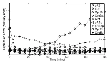
2.1 Simulated data from Cantoneet al.[2009] and Swat et al.[2004] . . . 32

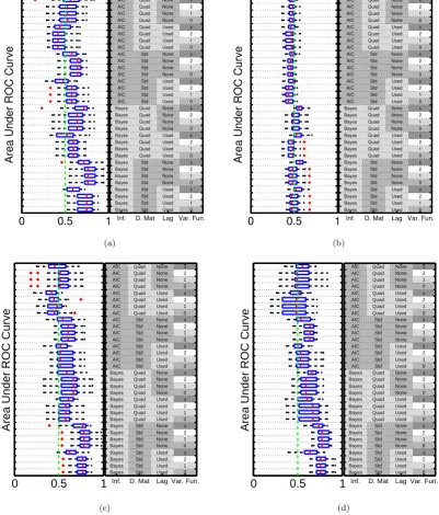
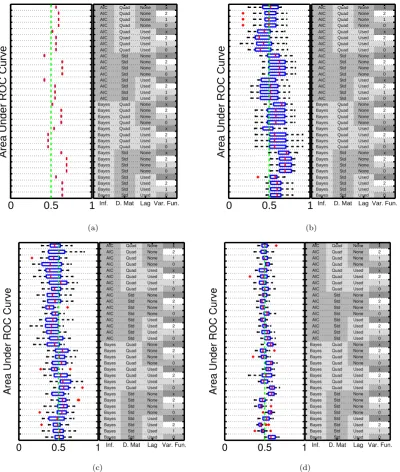
2.2 Network inference results (i) . . . 33

2.3 Network inference results (ii) . . . 34

2.4 Network inference results (iii) . . . 35

2.5 Network inference results (iv) . . . 36

2.6 Modelling variance as a function of the sampling interval . . . 37

3.1 Chemical Model Averaging (CheMA) . . . 43

3.2 Statistical models of enzyme kinetics . . . 44

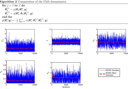
3.3 MCMC convergence diagnostics . . . 47

3.4 Sensitivity to hyper-parameter specification (i) . . . 49

3.5 Sensitivity to hyper-parameter specification (ii) . . . 50

3.6 Model of the MAPK signalling pathway . . . 50

3.7 Performance scores; AUPR and AUROC . . . 51

3.8 Prediction results; CheMA, simulation study . . . 53

3.9 Assessment of predictive performance . . . 53

3.10 Dynamical prediction for HCC 70 . . . 54

3.11 Prediction results; CheMA, breast cancer study . . . 55

3.12 (Marginal) parameter posterior distributions . . . 56

4.1 Epidermal growth factor receptor (EGFR) pathway . . . 61

4.2 Joint Network Inference (JNI) . . . 62

4.3 Hyper-parameter elicitation in JNI . . . 64

4.4 Insensitivity to the in-degree restriction . . . 70

4.5 Probing hyper-parameter sensitivity in JNI . . . 72

4.6 Investigating robustness to outliers and batch effects . . . 81

4.7 Network inference; JNI, breast cancer study . . . 83

4.8 Cell line specific networks inferred by JNI . . . 84

4.9 Two breast cancer cell lines from the same patient . . . 85

B.1 Data-generating ODE model . . . 95

B.2 Typical simulated time course . . . 96

(9)

List of Tables

2.1 Network inference schemes rooted in the linear model . . . 29

4.1 An example dataset for a single individualj, consisting of 3 variables, 2 time courses, each

with 4 time points. . . 65

4.2 Assessment of estimators for inference of individual networks Nj_{; autoregressive dataset}

with interventions . . . 73

4.3 Assessment of estimators for inference of the latent network N; autoregressive dataset

4.4 Assessment of estimators for inference of the network features; Autoregressive dataset

4.5 Assessment of estimators for inference of the latent network N; Autoregressive dataset

without interventions. . . 76

4.6 Assessment of estimators for inference of the individual networks Nj_{; Autoregressive}

dataset without interventions . . . 77

4.7 Assessment of estimators for inference of network features; Autoregressive dataset without

interventions . . . 78

4.8 Assessment of estimators for inference of the latent networkN; Xuet al.[2010] dataset . 79

4.9 Assessment of estimators for inference of individual networks; Xuet al.[2010] dataset . . 79

4.10 Assessment of estimators for inference of network features; Xuet al. [2010] dataset . . . . 80

B.1 Computational times . . . 97

(10)

Acknowledgements

This doctoral research was funded by the Engineering and Physical Sciences Research Council (EPSRC) through the Complexity Science Doctoral Training Centre and Department of Statistics at the University of Warwick (Coventry, UK). I am grateful to the Department of Biochemistry at the Netherlands Cancer Institute (Amsterdam, NL) for hosting my visit in the 2011-2012 academic year. The students and staff at each institution have made this study a pleasure.

Many people have had a direct impact upon this research, including Tarmo Aij¨o, John Aston,

Rod-erick Beijersbergen, Jen Bowskill, Thijn Brummelkamp, Quentin Caudron, Colm Connaughton, Frank Dondelinger, Joe Gray, Pantelis Hadjipantelis, Laura Heiser, Steven Hill, Kathy Jastrzebski, Steve Kid-dle, Theo Knijnenburg, James Korkola, Robert MacKay, Gordon Mills, Sergio Morales, Chris Penfold, Tassos Perrakis, Anas Rana, Phil Richardson, Monica Rigat, Gareth Roberts, Jordi Vidal Rodriguez,

Titia Sixma, Paul Spellman, Simon Spencer, Nicholas St¨adler, Vlad Vyshemirsky, Lodewyk Wessels,

Rachel Wilkerson and many anonymous referees.

In addition I am grateful to Stafford Library for providing an excellent writing environment and to Wikipedia for hastening the pace of this research.

(11)

Declaration

Parts of this thesis have been published or are in submission:

• Oates CJ, Mukherjee S (2012) Network Inference and Biological Dynamics. Ann. Appl. Stat.

6(3):1209-1235.

• Oates CJ, Hennessy BT, Lu Y, Mills GB, Mukherjee S (2012) Network Inference Using Steady

State Data and Goldbeter-Koshland Kinetics. Bioinformatics28(18):2342-2348.

• Oates CJ, Mukherjee S (2012) Causal Variable Selection Using Equilibrium Relations from

Non-linear Dynamics. Workshop on Causal Structure Learning, Uncertainty in Artificial Intelligence

(UAI’12). Santa Catalina, CA, USA.

• Oates CJ, Dondelinger F, Bayani N, Korkola J, Gray JW, Mukherjee S (2013) Network Inference

and Dynamical Prediction Using Biochemical Kinetics. In submission.

• Oates CJ, Korkola J, Gray JW, Mukherjee S (2012) Joint Estimation of Multiple Exchangeable

Networks. In revision.

(12)

Summary

Cellular response to a changing chemical environment is mediated by a complex system of interactions involving molecules such as genes, proteins and metabolites. In particular, genetic and epigenetic varia-tion ensure that cellular response is often highly specific to individual cell types, or to different patients in the clinical setting. Conceptually, cellular systems may be characterised as networks of interacting components together with biochemical parameters specifying rates of reaction. Taken together, the net-work and parameters form a predictive model of cellular dynamics which may be used to simulate the effect of hypothetical drug regimens.

(13)

Notation

This thesis assumes knowledge of standard mathematical and statistical notation. Application-specific notation aims to follow the conventions listed below. When convenient, these may be explicitly overlooked in order to simplify presentation.

N0 non-negative integers

R` non-negative reals

J “ t1, . . . , Ju index set of individuals, possibly biological samples

P “ t1, . . . , Pu index set of state variables

Xp chemical species associated with indexpPP

X˚

p phosphorylated form of speciesXp

G chemical reaction graph

N directed network

N discrete state vector inNP0

X continuous state vector inRP`

θ parameter vector

S, P, E substrate, product, enzyme respectively

Ep set of kinases acting on speciesXp

Ip,E set of inhibitors for kinaseEPEp

K Michaelis-Menten parameter

FX natural filtration of the stochastic processX

N Gaussian density / space of directed networks (depending on context)

KK statistical independence

Dpvq diagonal matrix with diagonal entriesv

y data, possibly corrupted by measurement noise

(14)

Introduction

The last two decades have seen rapid advances in biotechnology, enabling increasingly precise quan-titative measurement of molecular species in biological samples. In the 1990s the introduction of the DNA microarray facilitated the simultaneous and rapid quantification of RNA abundance for multiple

genes (Fig. 1). Comparison of these gene expression data across multiple biological samples offered an

unbiased approach to screen for genes which are statistically implicated (differentially expressed) in a

biological context of interest, relative to control samples. Microarray technology revolutionised funda-mental biological research by providing a mechanism by which to constrain experifunda-mental design, reducing the number of candidate genes for experimental investigation (e.g. knock-out or knock-down) [Crowther, 2002]. Translational research was also transformed, with gene expression data forming the basis for

several signatures which are predictive of response to therapy [van ’t Veeret al., 2002]. Subsequent years

saw the continued emergence of high-throughput biotechnologies, including array-comparative genomic hybridization (A-CGH), chromatin immunoprecipitation (ChIP) -on-chip DNA-binding assays, single-nucleotide polymorphism (SNP) arrays, high-throughput drug screening, protein microarrays and next generation sequencing. The increasing ease and decreasing cost of obtaining large amounts of data on a

biological system have led to an emphasis on integrative,systems level analysis. This paradigm is central

to the field of oncology, where it has become apparent that cancer is an emergent disease resulting from interplay between the functional effects of genetic or epigenetic mutations [Weinberg, 2007].

Multivariate biological data present significant challenges for modelling, computation and statistical interpretation. The need to analyse large biological datasets has sparked much interest in multivariate

and high-dimensional statistics [B¨uhlmann and van de Geer, 2011]. The visual representation of interplay

in a multivariate system which is afforded by a graph or network has proven extremely popular. A (standard) biological network consists of a set of nodes, representing molecular species such as genes, proteins or metabolites, and a set of edges which describe interactions or interplay between the nodes. Often attention is restricted to one particular form of molecular species (e.g. genes) and one form of interaction (e.g. transcriptional regulation). The type of molecular species which form the set of nodes and the biological mechanism which is encoded by the edges will lend its name to the network, so that we speak of gene regulatory networks, protein signalling networks or metabolic interaction networks, for example. Experimentalists have elucidated network topology for important biological processes, but the inherently combinatorial nature of networks provides a fundamental barrier to elucidating large amounts of topology on an edge-by-edge basis. The automatic characterisation of biological networks from high-throughput data obtained in a context of interest, such as a tissue type or a disease state, has become a prominent research goal in systems biology.

Cancer is a prevalent disease, with more than 1 in 3 people in the UK developing some form of cancer during their lifetime. Due in part to an ageing population, cancer incidence rates in Great Britain have risen by 22% in males and by 42% in females since the mid-1970s. Worldwide in 2008, there were estimated to be around 7.6 million cancer-related deaths and 12.7 million new cases. Intensive research on an international scale has led to advances in cancer therapeutics, such that cancer survival rates in the UK have doubled in the last 40 years. (All statistics taken from Cancer Research UK [2013] on 17/04/2013.)

One of the biggest scientific achievements of the last decade was the development of targeted anti-cancer drugs, which have demonstrated potential to revolutionise clinical treatment of the disease [Sud-hakar, 2009]. For example Imatinib (Novartis Pharma AG [2006] trade name Glivec) has rendered a subset of otherwise terminal leukaemia into a manageable chronic condition by targeting a tyrosine

ki-nase enzyme, known as BCR-ABL, which exists only in cancer cells and not in healthy cells [Moen et

al., 2007]. (Only a small minority of patients will acquire resistance to Imatinib [Mauro, 2006]).

(15)

[image:15.595.193.462.205.545.2]

Figure 1: The first reported use of miniaturized microarrays for gene expression profiling appeared in

Schena et al. [1995]. In total 45 genes were measured in Arabidopsis. Two years later Lashkari et al.

[1997] reported an assay of 2,479 genes in the yeastS. Cerevisiae. Modern microarrays can contain up

to 47,000 genes (e.g. Affymetrix GeneChip Human Genome U133 Plus 2.0). [Figure reproduced with

(16)

has dropped to an all time low [Silverman, 2012]. Experimental evidence suggests that many patients

become resistant to therapy via activation of secondarysurvivalpathways which were not targeted by the

original treatment [Leeet al., 2012]. Effective inhibition of these secondary pathways would be expected

to have a significant benefit for patients [Wetterskog et al., 2013]. The shift from mono-therapeutics

to poly-therapeutics necessitated by the complex, multivariate nature of cancer has, in part, driven the move towards systems biology.

A systems-level understanding of biological signalling processes introduces major experimental, trans-lational and theoretical challenges. For example in oncology, prior to treatment it is currently extremely difficult to predict which pathways will require targeting in order to achieve maximum efficacy. It is practically infeasible to assess all possible combinations of drugs in the laboratory using cultured cancer cells. Indeed, whilst the number of available drugs is now large, the number of pairs of drugs is consid-erably bigger. Moreover, each pair of drugs might be applied in a different sequential order, at different doses, at different times, for longer or shorter treatment durations etc. In principle these difficulties could be averted with access to an accurate computational model of cellular signalling dynamics, since

then hypothetical drug regimens could be rapidly exploredin silico[Hopkins, 2008]. However this raises

several theoretical challenges and there is currently a methodological void for systems-level inference and prediction in cellular signalling systems.

Cellular signalling systems have been modelled in a variety of ways, including discrete logic models

[Bender et al., 2010], discrete time Markov processes such as dynamic Bayesian networks (DBNs) [Hill

et al., 2012a], Markov jump processes [Paulsson, 2005; Wilkinson, 2006], Gaussian processes [Honkela et

al., 2010], structural equation models (SEMs) [Liuet al., 2008], ordinary differential equations (ODEs)

[Chen et al., 2009; Schoeberlet al., 2002] and stochastic differential equations (SDEs) [Finkenst¨adt et

al., 2013]. Almost all models of cellular signalling are rooted in network representations, either explicitly

as in DBNs and SEMs, or implicitly as in ODEs and SDEs [Sokol and Hansen, 2013]. Relating these models to data is often challenging. In this setting there are two main problems; (i) inference of model parameters, such as reaction rates, and (ii) uncovering a network structure which adequately describes interplay in the biological system under study. Classically, much effort has been directed at the first problem of estimating kinetic parameters, such as reaction rates, from noisy experimental data on the

molecular species. The second problem, which is commonly referred to asnetwork inference, has received

relatively less theoretical attention. In many biological contexts the edge structure of the network may be uncertain (e.g. due to genetic or epigenetic alterations in disease states). Then, an important biological goal is to perform network inference in a context-specific manner [Ideker and Krogan, 2012], that is, using data acquired in the biological context of interest. The ability to accurately estimate context-specific network topology has potential to greatly accelerate progress within systems biology, pharmacology and

related disciplines [Csermely et al., 2013]. For example, protein signalling network structure has been

shown determine the response of cells to certain therapeutic interventions [Lee et al., 2012]. Advances

in high-throughput data acquisition have led to much interest in such data-driven characterization of biological networks.

This thesis aims to contribute advances in the data-driven estimation of biological networks. Focussing primarily on inference for protein signalling networks, the novel contributions of this thesis can be summarised as follows:

• Chapter 2,From Biological Dynamics to Network Inference:

– Motivated by tractable approximations of complex stochastic dynamical systems, a connection

is drawn between several existing network inference algorithms in terms of a unified statisti-cal model. This framework makes explicit the assumptions underlying each approach, with particular emphasis on time series data obtained at uneven sampling intervals.

– A comprehensive empirical investigation assessed 32 different network inference algorithms

from this unified family using both simulated and real datasets where the data-generating networks were known by design.

– Our results highlight critical issues regarding the treatment of uneven sampling intervals,

which are shown to significantly effect the algorithms’ performance.

– One statistical formulation is shown to perform favourably in most data generating regimes;

this is taken as a basis for subsequent methodological development in Chapter 3.

(17)

– A novel statistical framework is presented which integrates non-linear chemical kinetics into inference for protein signalling networks.

– For time course data, Monte Carlo computation of model selection criteria is leveraged to

compute Bayes factors for non-linear dynamical systems defined on a network. Inference over networks is facilitated by Bayesian model averaging.

– Empirical investigations demonstrate improved network reconstruction on both simulated and

real datasets in comparison to approaches rooted in linear dynamical formulations.

– The methodology is demonstrated to be able to predict the effect of held-out interventions,

both in silico and in vitro. In particular the methodology facilitates prediction of cellular response in the challenging setting where neither the chemical reaction network, nor the

corresponding parameters are knowna priori.

• Chapter 4,Joint Estimation of Multiple Networks from Time Course Data:

– It is often the case that data are collected on multiple individuals j P J which may differ

with respect to interplay between variables. For example, in biology, different cell lines may possess differing protein signalling networks. A hierarchical Bayesian framework is proposed for joint inference in this setting.

– Unlike previous proposals, which were computationally prohibitive, an efficient, exact Bayesian

algorithm is proposed for reporting posterior marginal inclusion probabilities in the hierarchi-cal setting.

– A comprehensive study of joint estimation is undertaken, demonstrating how joint models

may yield improved network inference results bothin silicoandin vitro, using data obtained

from a panel of breast cancer cell lines.

(18)

Chapter 1

Background Material

Scientific investigation of complex systems increasingly requires a broad tool-kit of analytic, computa-tional and experimental techniques. This thesis assumes a background in both mathematics and statis-tics; in particular we will make use of differential equations, dynamical systems, stochastic processes, Bayesian statistics and Markov chain Monte Carlo. To a lesser extent we assume a basic understanding of cellular biology, including gene regulation and protein synthesis. In this Chapter we build on these bases in order to familiarise the reader with concepts necessary to follow the remainder. In particular we will discuss protein signalling mediated by phosphorylation, aberrant protein signalling in cancer, emerging experimental platforms, mathematical formalisms for chemistry, graphical models in statistics and a theory of inferred causation.

1.1 Biological Background

In this Section we introduce the fundamental biochemical process of protein signalling mediated by phosphorylation, discuss aberrant signalling in genetic diseases such as cancer, and describe some modern approaches to therapy which exploit the biochemistry of phosphorylation. Throughout we explicate these concepts in the context of well characterised signalling pathways in mammalian cells.

1.1.1 The (Not So) Central Dogma

Cellular response to a changing environment is mediated by a complex system of interactions involving

molecules such as genes, proteins and metabolites. The central dogma of molecular biology provides a

powerful constraint on the form of these interactions by specifying that certain information transferral processes are generally uni-directional [Crick, 1970]. In the language of graphical models, the central dogma postulates a set of conditional independences, as can be seen in Fig. 1.1. Specifically, the central

dogma implies that (i) DNA may be transcribed into RNA but generally notvice versa(ii) RNA may be

translated into protein molecules but generally notvice versaand (iii) proteins may regulate transcription

of RNA by binding to promoter regions (such proteins are known astranscription factors).

Since Crick’s description of the central dogma in 1970 it has become increasingly clear that many molecular interactions operate outside this paradigm; for example the post-translational modification of proteins (see Sec. 1.1.2) was not explicitly covered by the central dogma. This thesis focuses primarily on such interactions between protein molecules. However it is important to appreciate that these interactions are embedded in wider cellular signalling processes and are not generally causally sufficient (see Sec. 1.4.2).

1.1.2 Protein Signalling

(19)

[image:19.595.238.413.70.222.2]

Figure 1.1: Central dogma of molecular biology, reproduced from the original paper of Crick [1970].

particular we focus on a particular form of chemical change, known as protein phosphorylation, which plays an important role in aberrant protein signalling in cancer (see Sec. 1.1.3).

Definition 1(Phosphorylation). Phosphorylation is the addition of a phosphate (PO3´

4 ) group from a

high energy donor molecule, such as ATP, to a specific protein substrate, usually on the serine, threonine, or tyrosine amino acid (orresidue). When there is no ambiguity regarding the residue, the phosphorylated protein is simply referred to as a phosphoprotein.

Phosphorylation is an example of a post-translational modification (others being methylation, ubiq-uitylation, cleaving etc.). Post-translational modifications may alter a protein’s function or activity through a conformational change, for example enzyme phosphorylation may modulate catalytic activity by exposing/blocking the active domain. Phosphorylation is reversible and many residues on a protein may be phosphorylated (the p53 protein contains more than 18 different phosphorylation sites).

Definition 2(Kinase and phosphatase). Enzymes which catalyse phosphorylation are known as kinases, whilst enzymes which catalyse dephosphorylation are known as phosphatases.

Both kinases and phosphatases are typically highly specific, thereby exerting very precise control over cellular function. In many cases phosphorylation induces an activation of functionality, though this is not true in general, with counter examples including the retinoblastoma protein Rb which becomes inactive when phosphorylated. Often kinases and phosphatases are themselves phosphorylated proteins, so that an interconnected network of protein phosphorylation operates. Certain sub-networks have received much attention from the biological community - these well studied systems are typically referred to as “pathways”. Below we present a detailed example of a protein signalling pathway.

(20)

[image:20.595.44.503.213.543.2]

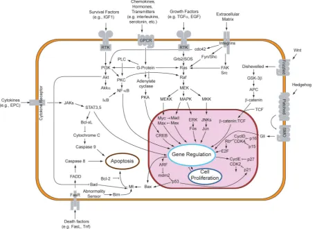
Figure 1.2: Schematic description of well-characterised signalling pathways in mammalian cells. Trans-membrane receptors (grey) such as receptor tyrosine kinases (RTKs) receive an external chemical sig-nal and transmit this through to the nucleus (purple) via a sequence of chemical reactions known as “signalling”, involving kinases such as MAPK and Akt. [“Overview of signal transduction pathways.”

(21)

[image:21.595.218.439.71.280.2]

Figure 1.3: Hallmarks of Cancer. These 10 characteristics are believed to be necessary conditions for cancer to occur; hence each represents a unique opportunity for targeted anti-cancer therapies. [Figure adapted from Hanahan and Weinberg [2011].]

1.1.3 Protein Signalling and Cancer

Multiple studies have demonstrated the remarkable genomic heterogeneity of cancer [The 1000 Genomes Project Consortium, 2010; The Cancer Genome Atlas Network, 2012]. Nevertheless there are a collection of concepts which provide justification for a unified theory of cancer. In particular Hanahan and Weinberg [2011] defined ten “hallmarks” which represent necessary criteria for a disease to manifest as cancer in the clinical setting (Fig. 1.3). Several of these hallmarks, such as sustained proliferative signalling, evading growth suppressors and resisting cell death, may be facilitated by aberrant protein signalling,

including signalling mediated by phosphorylation [Lee et al., 2012; Moen et al., 2007]. Thus protein

phosphorylation plays a leading role in oncogenesis.

In the context of cancer, there are three classes of gene which have become paradigmatic [Vogelstein and Kinzler, 2004].

Definition 3 (Oncogene, tumour-suppressor and stability genes). Proto-oncogenes, when mutated, be-come constitutively active (oncogenes) or active under conditions in which the wild-type gene is not.

Tumour-suppressor genes are targeted in the opposite way by genetic alterations; mutations reduce the

activity of the gene product, leading to tumour development. Stability genes (or caretaker genes) keep genetic alterations to a minimum; thus when they are inactivated, mutations in other genes occur at a higher rate, including mutations in proto-oncogenes and tumour-suppressor genes.

Example 2(MAPK pathway). Uncontrolled growth is a prerequisite for the development of all cancers [Hanahan and Weinberg, 2011]. In many cancers, a defect in the MAPK pathway leads to that uncon-trolled growth. For example, the proto-oncogene BRAF (whose role in MAPK signalling is becoming increasingly understood [Xu et al., 2010]) is known to be causally implicated in melanoma [Flaherty et al., 2010], with approximately 80% of cases involving a BRAF mutation.

Example 3 (Akt pathway). A key hallmark of cancer is resistance to cell death. In “wild type” cells, programmed cell death (apoptosis) is induced by either extracellular signals (inc. toxins, hormones, growth factors etc.) or intrinsic signals (inc. DNA damage). Apoptosis is an important defence against abnormal cellular behaviour and is disabled in cancer states. Akt (Fig. 1.2) is a key inhibitor of apoptosis which must be phosphorylated in order to be active. Phosphorylation of Akt is in turn regulated by PI3K; a protein frequently constitutively active in breast cancer (see Example 4 or Korkola et al. [2013]). Through over activation, PI3K provides a route for cancer cells to evade apoptosis.

(22)

into basal, luminal or claudin-low subgroups, whilst histological staining is used to explore the expression of

human epidermal growth factor receptor 2 (HER2),oestrogen receptor(ER) and progesterone receptor

(PR) [Sotiriou and Pusztai, 2009]. In total there are five “intrinsic” subtypes of breast cancer; luminal

A,luminal B,HER2-enriched,basal-likeand claudin-low[Eroles et al., 2012], though this classification

is disputed [Curtis et al., 2012]. In addition, genetic markers are used to further stratify biological samples. For example PIK3CA is a proto-oncogene which is mutated in 33% of breast cancer patients [Cizkova it et al., 2012]. Mutation renders its protein product PI3K constitutively active, meaning that it is no longer under the influence of receptor tyrosine kinases (RTKs; Fig. 1.2). HER2, another well known proto-oncogene, is amplified in approximately 30% of breast cancers. A frequently mutated tumour suppressor in many cancers is the TP53 gene [The Cancer Genome Atlas Network, 2012]. BRCA1 and BRCA2 are stability genes which assist in DNA repair pathways. Certain germ-line mutations in BRCA genes, common in certain population groups including Ashkenazi Jews, associate with an increased breast cancer risk. For example, women with an abnormal BRCA1 or BRCA2 gene have up to a 60% risk of developing breast cancer by age 90 [Breastcancer.org, 2012].

1.1.4 Targeted Cancer Therapies

Molecular cancer therapies may broadly be divided into targeted and untargeted therapies. A targeted therapy is a type of medication which blocks the growth of cancer cells by specifically interfering with molecules needed for carcinogenesis and tumour growth. In contrast, an untargeted therapy interferes with all rapidly dividing cells (e.g. traditional chemotherapy). In practice, patients are often treated

with a combination of both targeted and untargeted therapies [Carlson et al., 2009].

Each of the hallmarks of cancer (Fig. 1.3) defines, in principle, a set of targets for therapeutic inter-vention. In this thesis we are primarily concerned with interventions which tackle sustained proliferative signalling and evasion of apoptosis; in particular interventions which tackle aberrant protein phosphory-lation in the MAPK and Akt pathways (Examples 2,3). In this context there are two main molecular weapons; small molecule inhibitors and monoclonal antibodies.

Definition 4 (Small molecules). Small molecules are molecules with a low molecular weight (ă 800

Daltons) which enables them to rapidly diffuse across cell membranes in order to reach intracellular sites of action. In pharmacology, small molecules may bind to a protein and act as an effector, thereby altering the protein’s activity or function.

Example 5 (Small molecule kinase inhibitors). A protein kinase inhibitor is a type of small molecule inhibitor that specifically blocks the action of one or more protein kinases. Protein kinase inhibitors can be subdivided or characterised by the targets of the kinase whose activity is inhibited; most kinases act on both serine and threonine amino acids, the tyrosine kinases act on tyrosine, and a number (dual-specificity kinases) act on all three. Fig. 1.4 displays the 3D structure of EGFR inhibitor erlotinib, a reversible tyrosine kinase inhibitor.

Definition 5(Monoclonal antibodies). An antibodyis produced by the immune system in order to iden-tify and potentially neutralise foreign objects such as bacteria and viruses. Antibodies act by specifically binding to a target protein or cell type, thereby either tagging the target for attack by other parts of the immune system, or neutralising the target directly. Antibodies may be produced in large quantities in vitro for use in pharmacology. Monoclonalantibodies are antibodies derived from identical immune cells derived from a common ancestor.

Example 6 (Monoclonal antibodies in cancer). It is possible to design antibodies specific to almost any cell surface target. Tumour cells can display cell surface receptors that are absent or present in smaller quantities on the surfaces of healthy cells; often these are responsible for activating cellular signal transduction pathways that cause the unregulated growth and division of the tumour cell. Thus antibodies can be used to destroy malignant tumour cells and prevent tumour growth by blocking specific cell receptors. Examples include HER2, a constitutively active cell surface receptor that is produced at abnormally high levels on the surface of approximately 30% of breast cancer tumour cells. The monoclonal antibody Trastuzumab has been clinically approved to block the HER2 receptor in HER2 positive breast cancer patients [McKeage and Perry, 2002].

(23)

Figure 1.4: The 3D structure of EGFR inhibitor Erlotinib, a reversible tyrosine kinase inhibitor (source: www.rcsb.org; 1M17.pdb). Here the inhibitor (purple) binds to the epidermal growth factor receptor (EGFR; blue) in the ATP binding site, preventing catalytic activity.

an inhibitor of the Raf kinase. Now dozens of treatments for molecular players in this pathway are under clinical investigation [Roberts and Der, 2007]. For example, Fig. 1.4 shows how Erlotinib, a small molecule inhibitor of EGFR, can reduce catalytic activity by blocking the ATP binding site.

Example 8 (Small molecule inhibitors in breast cancer). Over-expression of HER2, ER or PR trans-membrane receptor proteins generally indicates that breast cancer cells are dependent on signalling down-stream of these receptors; in this case a natural strategy is to inhibit these receptors [Carlson et al., 2009]. For example, the small molecule inhibitor Lapatinib is used in combination therapy for HER2 positive breast cancer [Korkola et al., 2013]. Lapatinib belongs to a family of tyrosine kinase inhibitors, each of which specifically targets proteins involved in phosphorylation. Other family members involved in clinical trials to treat breast cancer include Gefitinib [ClinicalTrials.gov, 2013a], Cabozantinib [ClinicalTrials.gov, 2013b] and Neratinib [ClinicalTrials.gov, 2013c].

1.2 Experimental Background

1.2.1 Cancer Cell Lines

There exist several experimental systems for the study of cancer, including real patients, mouse models

[Frese and Tuveson, 2007],ex vivo tissue samples [Burdallet al., 2003], cell lines [Neveet al., 2006], ex

celluloassays [Hsieh et al., 1997] and virtual screening [Shoichet, 2004]. This thesis restricts attention to cell line models of cancer, in particular cell lines derived from breast cancer patients. The use of cell lines offers a number of advantages over alternative model systems, in addition to several disadvantages. We discuss both below:

• Strengths:

– Cost. Initial purchase of cell lines will typically cost in the region of£500 -£1,000 [ATCC, 2013]. Once acquired, cells may be cloned in unlimited quantity.

– Speed. Human fibroblast cells, for example, take approximately 24 hours to divide, facilitating rapid experimentation. In contrast, mouse models require several months per generation, and often several generations of selective breeding to obtain a desired genetic profile.

– Convenience. Basic laboratory equipment is sufficient to handle and maintain cell culture.

– Variety. Due to the rapidly expanding catalogue of cell lines, it is possible to construct (or purchase) panels of lines which exhibits a relatively high degree of genetic heterogeneity.

(24)

– Regulation. Laboratory use of primary tissue culture requires patient approval [Burdallet al., 2003], whereas cell lines may be used without the permission of the patient donor.

– Reproducibility. Cell lines (also mouse models) are standardised, with (in principle) identical cell cultures available to researchers globally. This level of reproducibility is not possible in patient studies, for example.

• Weaknesses:

– Model misspecification. Cell lines (asim. ex celluloassays and virtual screening) are far

re-moved from the relevantin vivo setting. In particular, (i) cell cultures typically occupy only

two spatial dimensions (although 3D is arriving, e.g. [Hsiaoet al., 2012; Souza et al., 2010])

(ii) the media in which cells are grown may differ from the relevant tumour micro-environment

[Aryaet al., 2012] (iii) cell lines are, by definition, immortalised; thus cell lines have been

se-lected for a genetic profile which is amenable to immortalisation (iv) the experimental set-up is idealised, so that otherwise challenging clinical aspects such as drug delivery or immunological response to therapy are ignored.

– Lineage. Many established breast cancer cell lines were not derived from primary breast tu-mours, but from tumour metastases. In particular, cell line catalogues tend to over-represent the more aggressive, metastatic, late-stage tumours, rather than the primary lesion. Since

most drug therapies are directed against the primary tumour [Burdallet al., 2003], this

con-tributes to the problem of model misspecification.

– Contamination. Cell line cross-contamination can be a problem for scientists working with cultured cells; indeed, studies suggest up to 15-20% of cells used in experiments have been

misidentified or contaminated with another cell line [Cabreraet al., 2006]. In particular the

HeLa cell line (the first cell line to be developed in 1952, from a glandular cancer of the cervix)

was notorious as a cross-contaminant [Nelson-Rees et al., 1981]. More recently, of 252 new

cell lines deposited at the German Cell Line Bank, 18% were found to be cross-contaminated [Masters, 2000]. This has led to a drive to define standardised procedures for verification of cell line identity [Masters, 2001].

– Mutation. Cell lines are prone to genotypic and phenotypic drift during their continual culture. This is particularly common in older and more frequently used cell lines. Sub-populations may arise and cause phenotypic changes over time by the selection of specific, more rapidly growing clones within a population. It has been demonstrated that MCF-7 cells (the most commonly used breast cancer cell line) show markedly different karyotypes (number and appearance of

chromosomes in the nucleus) between different UK laboratories [Bahiaet al., 2002; Osborne

et al., 1987]

– Growth. Maintaining cells in culture is non-trivial, with precise control required over

temper-ature, CO2levels, the growth medium and the plating density. Common pitfalls in this area

include nutrient depletion, accumulation of dead cells, contact inhibition (where over-crowding induces the inhibition of signalling processes) and cellular differentiation.

Cell lines have been widely used to investigate aberrant signalling processes in cancer. These studies

have included identification of bio-markers which are predictive of drug response [Heiser et al., 2011;

Korkolaet al., 2013], structure learning of signalling networks [Benderet al., 2010; Hillet al., 2012a] and

the identification of optimal drug combinations [Iadevaiaet al., 2010; Nelanderet al., 2008]. Coordinated

efforts to obtain data over hundreds of cancer cell lines [Barretina et al., 2012] provide an excellent

resource for such scientific enquiry.

1.2.2 Proteomics

Once an experimental system is available, it becomes necessary to accurately quantify the molecular profiles displayed by a phenotype of interest. For cell lines, there exist several platforms which can be used for analysis of protein phosphorylation, including Western blot [Burnette, 1981], enzyme-linked immunosorbent assay (ELISA; Engvall and Perlmann [1971]), mass spectrometry [Choudhary and Mann,

2010; Harsha and Pandey, 2010; Nita-Lazaret al., 2008], flow cytometry [Herzenberget al., 2002; Perez

(25)

[2001]) and Luminex [Duet al., 2008]. An excellent review of these methods can be found in Hill [2012a]. This thesis restricts attention to RPPA, which we discuss in detail below.

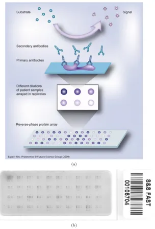
RPPA, first introduced in Paweletz et al. [2001], is an experimental platform for the quantitative

measurement of (phospho)protein abundance in biological samples. The reverse phase format operates in three stages (Fig. 1.5(a)): Firstly, an individual test sample (e.g. a cell lysate) is immobilised in an individual array spot. Secondly, the slide is incubated with a primary antibody that binds specifically to the protein of interest. Finally, this antibody is detected using a labelled secondary antibody (as in ELISA and Western blot) and subsequent signal amplification.

The above description is deliberately simplified and in practice experimental designs will be more complex. A protein microarray slide contains many spots which are grouped into batches, with these batches arranged in a grid (Fig. 1.5(b)), allowing for multiple samples to be immobilised and tested simultaneously. Probing multiple arrays (spotted with the same lysate) with different antibodies provides the effect of generating a multiplex readout. In practice, however, bandwidth is reduced since an entire batch must be allocated to testing of a single biological sample, due to the need to obtain dilution series (discussed below), in addition to technical replicates. Full details of RPPA protocol can be found in

[Hennessyet al., 2010; Tibeset al., 2006].

Protein concentrations and levels of phosphorylation can vary greatly, so accurate measurement over

a widedynamic range is required. The dynamic range of measurements is extended by diluting each

sample several times (at a known dilution ratio) and spotting onto the array at each dilution step. Hence, if the protein concentration in the original undiluted sample is near saturation, it can still be detected in the diluted samples. Fig. 1.5(b) displays batches containing eight-step dilutions in duplicate. Dilution series also aid the accurate quantification of protein concentrations by increasing the effective statistical sample size. Quantification is usually carried out using response curves which relate observed signal intensities to protein concentrations. The fact that a single antibody is used for the whole slide motivates the use of a single response curve for all samples on the slide. For the RPPA data used in this

thesis, a logistic model was used for the response curve (R packageSuperCurve [Huet al., 2007]).

We briefly summarise the strengths and weaknesses of the RPPA platform in relation to alternative technologies:

• Strengths:

– Reproducibility. Careful analysis of technical error by Hennessyet al. [2010] concluded that each of (i) between-batch, (ii) between-slide and (iii) between-run error variances were “low” compared to signal.

– High throughput. Multiple slides can be used to probe for multiple (phospho)proteins; tens or hundreds of proteins are often measured in the same experiment, providing an advantage over low-bandwidth techniques such as flow cytometry and live cell imaging.

– Sensitivity. RPPA is highly sensitive, requiring small amounts of sample to enable detection

of analytes; only 103_{cells are required for an RPPA experiment, compared with 10}8_{for mass}

spectrometry and 105 for Western blotting [Ramaswamyet al., 2005].

– Applicable. Denatured lysates (proteins which have lost their three-dimensional conformation) may be assayed, allowing antibodies to bind that previously would not have been able to do so, providing an advantage over tissue microarrays.

• Weaknesses:

– Antibody availability. The main limitation of RPPAs is the availability of sufficiently specific primary and secondary antibodies. Specificity is crucial for RPPA, since the signal from a spot could be due to cross-reactivity from unspecific binding and it is not possible to determine if this is the case from the data themselves. Therefore antibodies have to be carefully validated

by Western blotting prior to their use in RPPA assays [Hennessyet al., 2010]. The number of

(26)

(a)

[image:26.595.122.427.140.589.2]

(b)

Figure 1.5: (a) Reverse phase protein arrays operate in three stages. Firstly, an individual test sample (e.g. a cell lysate) is immobilised in an individual array spot. Secondly, the slide is incubated with a primary antibody that binds specifically to the protein of interest. Finally, this antibody is detected using a labelled secondary antibody (as in ELISA and Western blot) and subsequent signal amplification. (b) A typical reverse-phase protein array with 40 samples shown as the 40 batches on the slide. Each batch represents one individual sample with 16 spots, which are the results of duplicates of eight-step

(27)

– Aggregate data. Unlike flow cytometry and live cell imaging, RPPA provides no quantification

of single-cell variation, since many (ě 103_{) cell lysates are required to generate a read-out.}

Moreover, the population over which measurements are obtained contains cells which may not be synchronised with respect to signalling processes. Experimental protocol (Section B.6.1) partially synchronises cells by starvation followed by simultaneous stimulation, however the extent to which this strategy succeeds is unclear. Consequently, only population-average expression data is obtainable, which may compromise causal inference due to Simpsons’-type confounding.

– Batch effects. RPPA data are susceptible to batch effects; in particular, batch effects relating to a single slide are possible, so that a good experimental design will involve slide-slide control mechanisms.

– Relative quantification. Protein expression is quantified in relative terms between samples. It is therefore not possible to estimate absolute concentrations.

– Destructive sampling. Time course data is necessarily non-longitudinal due to the destructive observation process, leading to increased variability between temporally neighbouring samples.

– Low frequency. Due to manual preparation of the biological samples, it is difficult to achieve high temporal resolution using RPPA. For instance the time course data analysed in Chapter 3 have maximum time resolution of 30 minutes, although it is practically possible to sample up to 5 minute intervals. Compared to certain phosphorylation mechanisms, which can last mere seconds, this resolution may preclude identification of rapid signalling events.

The application of RPPA within cancer biology has recently been reviewed by Hill [2012a] and is reproduced below:

RPPAs have been used to investigate cancer cell signalling, both in cancer cell lines

[Hill et al., 2012a; Tibes et al., 2006] and in primary tumour samples [Malinowsky et al.,

2012; Sheehan et al., 2005]. These studies include the profiling and comparison of active

signalling pathways in different contexts; for example, between primary and metastatic

tu-mours [Quint´as-Cardama et al., 2012; Sheehan et al., 2005; Telesca et al., 2011] or between

cancer subtypes [Boydet al., 2008; Gujral et al., 2012; York et al., 2012], the identification

of signalling bio-markers that are predictive of response to certain anticancer agents [Boyd

et al., 2008], the identification of optimal drug combinations [Iadevaiaet al., 2010; Lavezzari

et al., 2012] and structure learning of signalling networks [Bender et al., 2010; Pierobonet

al., 2012]. For further studies see, for example, [Huet al., 2007; Spurrieret al., 2008; Zhang

and Pelech, 2012] and references therein. RPPAs have promising utility in the development

of personalised therapies [Pierobon et al., 2012]; using RPPAs to investigate and compare

signalling profiles in patient tumour cells and normal cells and to monitor changes in

phos-phorylation through time, both pre- and post-treatment [Lavezzariet al., 2012], could provide

information that guides the discovery and application of targeted therapies. Indeed, RPPAs

have recently been involved in several clinical trials (e.g. Beasley et al.[2012]; Davies et al.

[2012]; Muelleret al.[2010]).

1.3 Chemical Background

In this Section we formalise the idea of a system of chemical reactions, describe convenient approximations to the dynamics as the volume of the system increases and briefly survey the state-of-the-art statistical approaches to inference for such systems

1.3.1 Continuous Time Markov Processes

LetNiptq PN0denote the number of molecules of protein speciesXi,iPP “ t1, . . . , Pu, present at time

(28)

[image:28.595.52.492.81.460.2]

Figure 1.6: Chemical reaction graphGfor the MAPK signalling pathway; reproduced from Schoeberlet

al.[2002]. [Reaction ratesviare shown in green and reactants are shown in black. Hyphens are used to

indicate chemical complexes and arrows indicate the reaction topology.]

Definition 6 (Chemical reaction graph). Achemical reaction graphis a system ofv chemical reactions

R1, . . . ,Rv with rate constants k1, . . . , kv and reaction coefficientspij, qij PN0:

R1:p11X1`p12X2` ¨ ¨ ¨ `p1PXP k1

ÝÑ q11X1`q12X2` ¨ ¨ ¨ `q1PXP

R2:p21X1`p22X2` ¨ ¨ ¨ `p2PXP k2

ÝÑ q21X1`q22X2` ¨ ¨ ¨ `q2PXP ..

.

Rv:pv1X1`pv2X2` ¨ ¨ ¨ `pvPXP kv

ÝÑ qv1X1`qv2X2` ¨ ¨ ¨ `qvPXP

Here the reaction coefficientspij, qij are non-negative integers, since only entire molecules may react.

Collecting together reaction coefficients produces matrices P,Q P Nv0ˆP whose transposed difference

S “ pQ´PqT PN0Pˆv is known as thestoichiometry matrix. Theith columnsi ofS is then the state

change vector for reaction _Ri, quantifying the net change in protein quantities as a result of reaction

Ri occurring. Fig. 1.6, reproduced from Schoeberl et al. [2002], contains a chemical reaction graph

representation for the MAPK pathway. Note that the use of “graph” here is non-standard, motivated by a graphical representation of kinase-substrate reactions which we will exploit in Chapter 3.

(29)

if for alln,n1_P

NP0 there existsqn,n1 P_R_` such that PpNpt`δtq “n1

|Nptq “nq “qn,n1δt`opδtq. (1.1)

Theqn,n1 are known as transition rates.

Definition 8 (Mass action kinetics). Under (stochastic) mass action kinetics the state vector N is a continuous time Markov process with transition rates given by

qn,n1 “

ÿ

i

Itn´n1“siuhipnq (1.2)

where

hipNq “ki

ź

j

ˆ

Ni

pij

˙

(1.3)

is the hazardof reaction _Ri occurring.

Mass action kinetics assumes a well-mixed chemical population and sufficiently large numbers of reactants; these assumptions must be carefully assessed in real biological systems [Sayikli and Bagci, 2011]. Such dynamics are easily simulated using, for instance, the Gillespie algorithm [Wilkinson, 2006]. Using modern parallel processing technology, forward simulation is possible at computational complexity

OptlogpPqqwheretis the duration of the simulation andP is the number of biochemical species [Li and

Petzold, 2008].

1.3.2 Chemical Langevin Equation

Inference for continuous time Markov processes from discrete, noisy data is extremely challenging

[Wilkin-son, 2006]. One popular solution is to approximate the discrete variablesNiby continuous variables ΩXi

where Ω is the volume of the system andXi is the density or concentration ofXi. Two well known

ap-proximations of this form are the chemical Langevin equation (CLE) and the linear noise approximation (LNA); we derive both in the following Sections.

Theorem 1(Chemical Langevin equation). The continuous time Markov processNptqcan be approxi-mated byΩXptqwhere XPRP` satisfies the stochastic differential equation

dX“ÿ

i

hipXqsidt`?1

Ω ÿ

i

b

hipXqsidBi. (1.4)

wherehipXq “limΩÑ8Ω´1hiprΩXsq.

Sketch Proof: Consider a time intervalI“ rt, t`δtqwhereδtis sufficiently small that hazardshipNpsqq

are approximately constant for s P I. Then the number Ri of reactions Ri which occur during the

interval may be modelled using a Poisson random variableRi «„P opλiqwith mean λi “hipNptqqδt.

The diffusion approximation proceeds by using instead a GaussianRi «„ Nipλi, λiq whose mean and

variance are chosen to match those of the Poisson distribution. Thus we obtain

Npt`δtq ´Nptq «„ ÿ

i

NiphipNptqqδt, hipNptqqδtqsi (1.5)

“ ÿ

i

hipNptqqsiδt`

ÿ

i

a

hipNptqqsiNip0, δtq. (1.6)

Close to the thermodynamic limit (Ω´1_h

ipNq «hipXq) we may rewrite Eqn. 1.6 as

Xpt`δtq ´Xptq «„ÿ

i

hipXptqqsiδt`

1 ?

Ω ÿ

i

b

hipXptqqsiNip0, δtq. (1.7)

TakingδtÑ0 we then arrive at the chemical Langevin equation (CLE).

The Gaussian approximation to a Poisson density relies on the parametersλi“hiδtbeing sufficiently

(30)

δt of the interval is small. Thus it is not clear a priori whether such a regime exists. However it has been proven that the CLE is a good approximation to the stochastic dynamics whenever the system is

sufficiently close to the thermodynamic limit (Section 1.3.4) [Gillespie, 2009; Wallaceet al., 2012]. l

The CLE relaxes the assumption of discrete state space whilst preserving important behavioural features of the original continuous time Markov process, including conserved quantities such as total molecular concentrations. However the quality of the CLE approximation may deteriorate in situations where low concentrations are encountered, in which case the CLE underestimates the effect of stochastic fluctuations. Inference using the CLE has been studied by [Golightly and Wilkinson, 2011] who exploit efficient particle MCMC sampling strategies.

1.3.3 Linear Noise Approximation

Inference for SDEs remains challenging despite several recent advances in this area (e.g. Kalogeropoulos

et al.[2010]; Papaspiliopouloset al.[2012] and references therein), since in general the likelihood function is unavailable in closed form [Wilkinson, 2006]. An attractive approach is to develop a closed form approximation to the CLE; the LNA which we describe below is one well known example.

Noting that the CLE (Eqn. 1.4) differs to the macroscopic rate equation (Eqn. 1.12) by a term of

order 1{?Ω, we take the ansatz Xptq « µptq `ξptq{?Ω where µis the deterministic solution to the

macroscopic rate equation.

Theorem 2 (Linear noise approximation [van Kampen, 1976]). The solutionXptqof the CLE may be approximated byµptq `ξptq{

?

Ωwhere µis the deterministic solution to the macroscopic rate equation

dµ

dt “

ÿ

i

hipµqsi, µp0q “x0. (1.8)

and ξsatisfies the SDE

dξ“ÿ

i

Dµhipξqsidt`

ÿ

i

b

hipµqsidBi, ξp0q “0 (1.9)

where Dµhipξq “dhipµq{dµ¨ξ denotes the directional derivative of hi, evaluated at µ, in the direction

ξ.

Sketch Proof: Using a linear expansion of the hazardshipµptq `ξptq{

?

Ωqaboutµptqresults in

hi

ˆ

µptq `ξ?ptq Ω

˙

“hipµptqq `?1

Ω ÿ

j

fijptqξjptq `O

ˆ 1 Ω

˙

(1.10)

where fij “dhipµq{dµj. Upon substitution of our ansatz Xptq «µptq `ξptq{

?

Ω into the CLE (Eqn.

1.4) and using Eqn. 1.10 we obtain, up to _Op1{

?

Ωq, Eqn. 1.9. l

The law ofX under the LNA is encoded in the solution to Eqn. 1.9. Recently Wallace et al.[2012]

described how to solve Eqn. 1.9 exactly; specifically,ξptq „Np0,Σptqqis Gaussian in distribution where

covariance matrixΣ satisfies the following system of linear ODEs

dΣ

dt “SfΣ` pSfΣq

T

`SdiagphpµqqST (1.11)

subject to the initial condition Σp0q “0, where diagphqrepresents the diagonal matrix with diagonal

equal to h. Thus we may augment the macroscopic rate equation (Eqn. 1.8) with the covariance

equations (Eqn. 1.11) and jointly solve the system in order to obtain an exact distribution for the LNA of Xptq.

The LNA has recently received attention from the statistical and applied mathematics communities:

Komorowski et al. [2011] proposed using the LNA to approximate the Fisher information matrix for

stochastic chemical kinetics, thereby investigating sensitivity, robustness and identifiability of chemical

systems. Mugler et al.[2011] reverse-engineered biochemical networks which process signals according

(31)

In a similar way Finkenst¨adtet al.[2013]; Komorowski et al.[2009] used the LNA to uncover the rate parameters governing the expression of a single gene. Furthermore the theory has been extended in

several directions: Pahlajani et al. [2011] investigated extensions to the LNA for cases where reaction

rates induce separable time scales, overcoming potential stiffness of the associated ODEs. Challenger

et al. [2012] introduced spatial heterogeneity by extending the LNA to compartmentalised models of chemical interaction. Stathopoulos and Girolami [2012] demonstrated how to exploit manifold MCMC techniques for efficient inference under the LNA.

1.3.4 Thermodynamic Limit

In situations where the volume Ω of the system is large, concentrations of molecular species are not too

low, and the system is approximately well mixed, it may be desirable to model the processXptqas fully

deterministic. The thermodynamic limit allows molecular quantities Ni and the system volume Ω to

approach infinity together in such a way that concentrationsXi “Ni{Ω remain constant. In this limit

the concentrations may be shown to satisfy the continuous solution of the macroscopic rate equation

dX

dt “

ÿ

i

hipXqsi, Xp0q “x0. (1.12)

Mass action kinetics do not permit analytic solution, meaning that exact inference is typically facilitated

using forward-simulation (“likelihood free”) approaches, e.g. [Chen et al., 2009; Toni et al., 2009].

Nevertheless such simulation-intensive approaches do not lend themselves to rapid, interactive inference. In cellular biology the topology of chemical reaction graphs may be highly structured with an emphasis onmotifs which confer certain dynamical properties such as stability, feedback, or switch-like behaviour [Alon, 2007]. For several such motifs there exist a number of well-studied analytic approximations to the dynamics which may assist in modelling efforts. Below we describe some examples from enzyme kinetics which are central to this thesis.

Example 9(Michaelis-Menten kinetics). Michaelis-Menten kinetics is an approximation to mass actions kinetics which describes the conversion of a substrate_XS into a productXP under the catalytic activity of an enzyme_XE [Michaelis and Menten, 1913]. Specifically we seek to approximate the dynamics arising from the chemical reaction motif

XS`XE k1 é

k´1X

EXS Ñk2 XE`XP (1.13)

where standard shorthand notation encodes a system of v “3 chemical reactions; see Def. 6. Under mass action kinetics (below) the dynamical system corresponding to Eqn. 1.13 does not permit closed form solution:

dXS

dt “ ´k1XEXS`k´1XES (1.14)

dXE

dt “ ´k1XEXS` pk´1`k2qXES (1.15)

dXES

dt “ k1XEXS´ pk´1`k2qXES (1.16)

dXP

dt “ k2XES (1.17)

Michaelis-Menten kinetics state that the rate of production ofP is given approximately by

dXP

dt «

V XE0XS

XS`K

(1.18)

whereXE0 denotes the total concentration of enzyme (including molecules involved in the complexXES),

V is the maximal reaction rateandK is a Michaelis-Mentenparameter.

Eqn. 1.18 is an attractive alternative to the system of Eqns. 1.14-1.17 since only two parameters are required to characterise the dynamics. Moreover unlike mass action kinetics (Eqns. 1.14-1.17),