STOCK-MARKET FORECASTING USING MACHINE LEARNING
*Parag Hirulkar, Dipak Raut, Ashok Shinde, Anjali Jagtap
Department of Electronics and Telecommunication, International Institute of Information Technology
ARTICLE INFO ABSTRACT
Stock market process is fully uncertainty affected by many factor so that's anyone cannot predict stock market future to solve this problem construct the model which is gather all
data, analyze data according stock that predict stock market future hence stock market prediction is important extraction in finance and business. Examines the theory and practice of real time analysis techniques for prediction
The original pre
of currency values and financial ratios. The data formats in currency values a
provide a process for computation of stock prices. The transformed data set contains only a standardized ordinal data type which provides a process to measure rankings of stock price trends. The outcomes of both processes are examined a
analysis from machine learning software. This project focuses on using univariate time series forecasting methods for the stock market index, Standard Poor's 500 (abbreviated commonly as SP 500, whic
Moving Average (ARIMA) modelling. Time series analysis was through using R and R studio to both predict and visualize predictions. Along with the interactivity of
we were able to create stunning visuals that help in understanding which time series forecasting method is most appropriate for time series analysis.
Copyright©2017, Parag Hirulkar. This is an open access article
distribution, and reproduction in any medium, provided the original work is properly cited.
INTRODUCTION
From the beginning of time it has been mans common goal to make his life easier. The prevailing notion in society is that wealth brings comfort and luxury, so it is not surprising that there has been so much work done on ways to predict the markets. Various technical, fundamental, and statistical indicators have been proposed and used with varying results. However, no one technique or combination of techniques has been successful enough. With the development of neural networks, researchers and investors are hoping that the market mysteries can be unravelled. A stock market is a public market for the trading of company stock and derivatives at an agreed price; these are securities listed on a stock exchange as well as those only traded privately. It is an organized set
regulatory body and the members who trade in shares are registered with the stock market and regulatory body SEBI. The stock market is also called the secondary market as it involves trading between two investors. Stock market gets investors together to buy and sell their shares. Share market sets prices according to supply and demand.
*Corresponding author: Parag Hirulkar,
Department of Electronics & Telecommunication, International Institute of Information Technology
ISSN: 0975-833X
Article History:
Received 27th April, 2017 Received in revised form 30th May, 2017
Accepted 07th June, 2017 Published online 22nd July, 2017
Citation: Parag Hirulkar, Dipak Raut, Ashok Shinde, Anjali Jagtap and
International Journal of Current Research, 9, (07), 53503
Available online at http://www.journal
Key words:
Machine Learning, ARIMA,
Time series analysis.
RESEARCH ARTICLE
MARKET FORECASTING USING MACHINE LEARNING
Parag Hirulkar, Dipak Raut, Ashok Shinde, Anjali Jagtap and
Telecommunication, International Institute of Information Technology
ABSTRACT
Stock market process is fully uncertainty affected by many factor so that's anyone cannot predict stock market future to solve this problem construct the model which is gather all
data, analyze data according stock that predict stock market future hence stock market prediction is important extraction in finance and business. Examines the theory and practice of real time analysis techniques for prediction of stock price trend by using a transformed data set in ordinal data format. The original pre transformed data source contains data of heterogeneous data types used for handling of currency values and financial ratios. The data formats in currency values a
provide a process for computation of stock prices. The transformed data set contains only a standardized ordinal data type which provides a process to measure rankings of stock price trends. The outcomes of both processes are examined and appraised. The primary design is based on time series analysis from machine learning software. This project focuses on using univariate time series forecasting methods for the stock market index, Standard Poor's 500 (abbreviated commonly as SP 500, which is the notation used in this project) emphasizing on Box
Moving Average (ARIMA) modelling. Time series analysis was through using R and R studio to both predict and visualize predictions. Along with the interactivity of
we were able to create stunning visuals that help in understanding which time series forecasting method is most appropriate for time series analysis.
is an open access article distributed under the Creative Commons Attribution License, which distribution, and reproduction in any medium, provided the original work is properly cited.
From the beginning of time it has been mans common goal to make his life easier. The prevailing notion in society is that wealth brings comfort and luxury, so it is not surprising that there has been so much work done on ways to predict the s technical, fundamental, and statistical indicators have been proposed and used with varying results. However, no one technique or combination of techniques has been successful enough. With the development of neural hoping that the market mysteries can be unravelled. A stock market is a public market for the trading of company stock and derivatives at an agreed price; these are securities listed on a stock exchange as well as anized set-up with a regulatory body and the members who trade in shares are registered with the stock market and regulatory body SEBI. The stock market is also called the secondary market as it involves trading between two investors. Stock market gets estors together to buy and sell their shares. Share market
Department of Electronics & Telecommunication, International
Stocks that are in demand will increase their price, whereas as stocks that are being heavily sold will decrease their price. Companies that are permitted to be traded in this market place are called listed companies. Investors in stock market want to maximize their returns by buying or selling their investments at an appropriate time. Since stock market data are highly time variant and are normally in a nonlinear pattern, predicting the future price of a stock is highly challenging. With the increase of economic globalization and evolution of information technology, analyzing stock market data for predicting the future of the stock has become increasingly challenging, important and rewarding. Prediction provides knowledgeable information regarding the current status of
movement. Thus this can be utilized in decision making for customers in finalizing whether to buy or sell the particular shares of a given stock. Investor has often found it very costly to acquire useful information to assist them in inves decision making. For example, many investors have devoted a great deal of time to read messages posted on internet stock message boards to estimate asset prices based on information of varying quality. It has been reported that these message boards can have a significant impact on financial markets. Efficient investment decision making today is based on a variety of information sources including historical financial
International Journal of Current Research
Vol. 9, Issue, 07, pp.53503-53513, July, 2017
Parag Hirulkar, Dipak Raut, Ashok Shinde, Anjali Jagtap and Smita Kadam, 2017. “Stock-Market Forecasting using Machine Learning
53503-53513.
Available online at http://www.journalcra.com
z
MARKET FORECASTING USING MACHINE LEARNING
Smita Kadam
Telecommunication, International Institute of Information Technology
Stock market process is fully uncertainty affected by many factor so that's anyone cannot predict stock market future to solve this problem construct the model which is gather all information from historical data, analyze data according stock that predict stock market future hence stock market prediction is important extraction in finance and business. Examines the theory and practice of real time analysis of stock price trend by using a transformed data set in ordinal data format. transformed data source contains data of heterogeneous data types used for handling of currency values and financial ratios. The data formats in currency values and financial ratios provide a process for computation of stock prices. The transformed data set contains only a standardized ordinal data type which provides a process to measure rankings of stock price trends. The nd appraised. The primary design is based on time series analysis from machine learning software. This project focuses on using univariate time series forecasting methods for the stock market index, Standard Poor's 500 (abbreviated commonly as SP h is the notation used in this project) emphasizing on Box-Jenkins Autoregressive Integrated Moving Average (ARIMA) modelling. Time series analysis was through using R and R studio to both predict and visualize predictions. Along with the interactivity of plotly through the ggplot2 package we were able to create stunning visuals that help in understanding which time series forecasting
ribution License, which permits unrestricted use,
are in demand will increase their price, whereas as stocks that are being heavily sold will decrease their price. Companies that are permitted to be traded in this market place are called listed companies. Investors in stock market want to eturns by buying or selling their investments at an appropriate time. Since stock market data are highly time-variant and are normally in a nonlinear pattern, predicting the
tock is highly challenging. With the increase lization and evolution of information technology, analyzing stock market data for predicting the future of the stock has become increasingly challenging, important and rewarding. Prediction provides knowledgeable information regarding the current status of the stock price movement. Thus this can be utilized in decision making for customers in finalizing whether to buy or sell the particular shares of a given stock. Investor has often found it very costly to acquire useful information to assist them in investment decision making. For example, many investors have devoted a great deal of time to read messages posted on internet stock message boards to estimate asset prices based on information of varying quality. It has been reported that these message an have a significant impact on financial markets. Efficient investment decision making today is based on a variety of information sources including historical financial INTERNATIONAL JOURNAL OF CURRENT RESEARCH
data series and messages posted on stock message boards. There have been a number of studies showing that the sentiment contained in these messages has been correlated with stock prices. Moreover, many researchers claim that the stock market is a chaos system. Chaos is a non linear deterministic system which only appears random because of its irregular fluctuations. These systems are highly sensitive to the initial conditions of the systems. These systems are dynamic, a periodic, and complicated and are difficult to deal with normal analytical methods. The neural networks are effective in learning such non linear chaotic systems because they make very few assumptions about the functional form of the underlying dynamic dependencies and their initial conditions. This may eventually question the traditional financial theory of efficient market. Many researchers and practitioners have proposed many models using various fundamental, technical and analytical techniques to give a more or less exact prediction. Fundamental analysis involves the in-depth analysis of the changes of the stock prices in terms of exogenous macroeconomic variables. It assumes that the share price of a stock depends on its intrinsic value and the expected return of the investors. But this expected return is subjected to change as new information pertaining to the stock is available in the market which in turn changes the share price.
Apart from these commonly used methods of prediction, some traditional time series forecasting tools are also used for the same. In time series forecasting, the past data of the prediction variable is analyzed and modelled to capture the patterns of the historic changes in the variable. These models are then used to forecast the future prices. There are mainly two approaches of time series modelling and forecasting: linear approach and the nonlinear approach. Mostly used linear methods are moving average, exponential smoothing, time series regression etc. One of the most common and popular linear method is the Autoregressive integrated moving average (ARIMA) model (Box and Jenkins (1976)). It presumes linear model but is quite exible as it can represent different types of time series, i.e. Autoregressive (AR), moving average (MA) and combined AR and MA (ARMA) series.
Objective
The stock market processing is full of uncertainty and is affected by countless different factors. Hence the stock market prediction is one of the most important exertions for finance analysts and businessmen
Literature Survey
The techniques and developed facilities for exploiting especially financial news, social media data and analysis results are presented. A prediction model has been built that uses big data analytical capabilities, social media paralytics and machine learning to periodically predict the trend about stock markets. Model shows that sentiment analysis of the social data complements proven technical analysis methods such as regression analysis. It shows that volatility of the markets and the future performance of the system is affected by the economic and political news and of the social media. Exploiting social media data in addition to numeric data increases the quality of the input and gives improved predictions. The aide of big data technology allows predictions at real-time. However the algorithm used for sentiment analysis uses summative assessment of the sentiments in a particular news article or tweet, this could be improved for better
sentiment calculations, which would improve the accuracy of
the prediction (Bing et al., 2014). Analysis works especially on
public opinion taking from social media like twitter in this analysis used data mining algorithm they can discover pattern between public segment and stock market price.NPL classify tweet in 5 category, with help of that we analyse data, and probability of which output will come. using keyword we separate data from huge data more specifically proposed algorithm has defined the whole relationships embedded in social media as a graph with several layers proposed algorithms have a better prediction performance in some certain industries such as IT and media This knowledge should aid these companies to effectively manage or promote products and brands via sentiment management in social media (Keisuke
Mizumoto et al., 2012). It predicts a high percentage of the
outcomes for various stocks, and does not lose much accuracy when applied to a sample from outside the training sample. This model has great amount of room for improvement. Such improvement can be attained by adding additional variables, particularly those showing aspects of the company not related to profitability or earnings-share relationships. Multivariate statistics can be used to analyse a company's likely performance in the stock market with respect to global economic conditions as well as its own financial performance the previous year (Siew and Nordin, 2012). Polarity dictionary automatically using a semi-supervised learning and determine a polarity of stock market news using a constructed dictionary. Its confirm that the proposed method adds many words in a polarity dictionary and can determine correct polarities of all news. Moreover we confirm that the size of a polarity
dictionary is change as a threshold value varies (Zhen Hu et al.,
2013).
accuracy is an important yet often difficult task facing decision makers in many areas. Both theoretical and empirical findings have indicated that integration of different models can be an effective way of improving upon their predictive performance, especially when the models in combination are quite different. Artificial neural networks (ANNs) are flexible computing frameworks and universal approximates that can be applied to a wide range of forecasting problems with a high degree of accuracy. However, using ANNs to model linear problems have yielded mixed results, and hence; it is not wise to apply ANNs blindly to any type of data. Auto-regressive integrated moving average (ARIMA) models are one of the most popular linear models in time series forecasting, which have been widely applied in order to construct more accurate hybrid models during the past decade. Although, hybrid techniques, which decompose a time series into its linear and nonlinear components, have recently been shown to be successful for single models, these models have some disadvantages. In this paper, a novel hybridization of artificial neural networks and ARIMA model is proposed in order to overcome mentioned limitation of ANNs and yield more general and more accurate forecasting model than traditional hybrid ARIMA-ANNs models. In proposed model, the unique advantages of ARIMA models in linear modelling are used in order to identify and magnify the existing linear structure in data, and then a neural network is used in order to determine a model to capture the underlying data generating process and predict, using pre-processed data. Empirical results with three well-known real data sets indicate that the proposed model can be an effective way to improve forecasting accuracy achieved by traditional hybrid models and also either of the components models used
separately (Hyndman et al., 2012).
Proposed Methodology
Forecasting Methods
Some forecasting methods are very simple and surprisingly effective. Here are four methods that we will use as benchmarks for other forecasting methods.
Average Method
Here, the forecasts of all future values are equal to the mean of the historical data. Let the historical data be denoted by y1,
yTy1, yT then we can write the forecasts as
yT + h|T = y = (y1 + + yT)|T.yT + h|T = y = (y1 + + yT)|T
The notation yT + h|T yT + h|T is a short-hand for the estimate
of yT + hyT + h based on the data y1, yTy1, yT. Although we
have used time series notation here, this method can also be used for cross-sectional data (when we are predicting a value not included in the data set). Then the prediction for values not observed is the average of those values that have been observed. The remaining methods in this section are only applicable to time series data.
Naive Method
This method is only appropriate for time series data. All forecasts are simply set to be the value of the last observation. That is, the forecasts of all future values are set to be yTyT, where yTyT is the last observed value. This method works remarkably well for many economic and financial time series. R code naive(y, h) rwf(y, h) Alternative
Seasonal Naive Method
A similar method is useful for highly seasonal data. In this case, we set each forecast to be equal to the last observed value from the same season of the year (e.g., the same month of the previous year). Formally, the forecast for time T + hT + h is written as yT + hkm where m= seasonal period, k = (h1)/m + 1, yT + hkm where m= seasonal period, k = (h1)/m + 1,and uu denotes the integer part of uu. That looks more complicated than it really is. For example, with monthly data, the forecast for all future February values is equal to the last observed February value. With quarterly data, the forecast of all future Q2 values is equal to the last observed Q2 value (where Q2 means the second quarter). Similar rules apply for other months and quarters, and for other seasonal periods.
Exponential Smoothing
Exponential smoothing is a rule of thumb technique for smoothing time series data, particularly for recursively applying as many as three low pass filters with exponential window functions. Such techniques have broad application that is not intended to be strictly accurate or reliable for every situation. It is an easily learned and easily applied procedure for approximately calculating or recalling some value, or for making some determination based on prior assumptions by the user, such as seasonality. Like any application of repeated low-pass filtering, the observed phenomenon may be an essentially random process, or it may be an orderly, but noisy, process. Whereas in the simple moving average the past observations are weighted equally, exponential window functions assign exponentially decreasing weights over time. The use of three filters is based on empirical evidence and broad application. Exponential smoothing is commonly applied to smoothen data, as many window functions are in signal processing, acting as low pass filters to remove high frequency noise. This method parrots Poisson's use of recursive exponential window
functions in convolutions from the 19th century.
Random Walk Model
The random walk theory suggests that stock price changes have the same distribution and are independent of each other, so the past movement or trend of a stock price or market cannot be used to predict its future movement. In short, this is the idea that stocks take a random and unpredictable path.
R(t + 1) = R(t) + e
It basically states that returns on a stock tomorrow can be calculated using the return today plus an error term. An error term is the deviation of reality from model. If it was possible to be calculated, it should have been integrated into model.
Engle-Granger method
Is a statistical property of a collection (X1, X2, .., Xk) of time
series variables. First, all of the series must be integrated of order 1 (see Order of integration). Next, if a linear combination of this collection is integrated of order zero, then the collection is said to be co-integrated. Formally, if (X,Y,Z) are each integrated of order 1, and there exist coefficients a,b,c such that aX +bY +cZ is integrated of order 0, then X, Y, and Z are co-integrated. Co-integration has become an important property in contemporary time series analysis. Time series often have trends either deterministic or stochastic. In an influential paper,
Charles Nelson and Charles Plosser (1982) provided statistical evidence that many US macroeconomic time series (like GNP, wages, employment, etc.) have stochastic trends these are also called unit root processes, or processes integrated of order 1I(1). They also showed that unit root processes have non-standard statistical properties, so that conventional econometric theory methods do not apply to them.
Cross-Sectional Momentum Models
Cross-sectional momentum models rational models are, to some extent, related to binary response models. However, instead of estimating the probability of being in one bin of a dichotomous variable, the fractional model typically deals with variables that take on all possible values in the unit interval. One can easily generalize this model to take on values on any other interval by appropriate transformations. Examples range from participation rates in 401(k) plans to television ratings of NBA games. There have been two approaches to modelling this problem. Even though they both rely on an index that is linear in xi combined with a link function, this is not strictly necessary. The first approach uses a log-odds transformation of y as a linear function of xi, i.e,. This approach is problematic for two distinct reasons.
Among all the available methods mention random walk method accuracy is not accurate and do not analysis all the historic data. In Engle-Granger method, First of all, it identifies only a single co-integrating relation, among what might be many such relations. This requires one of the variables, to be identified as "first" among the variables in. This choice, which is usually arbitrary, affects both test results and model estimation. Prediction of stock market values is done by following method for less error and good accuracy.
Mean Forecast
Naive Forecast
Seasonal Naive Forecast
Exponential Smoothing Forecast
Existing system for prediction
There are two types of analysis possible for prediction, technical and fundamental.
Based on technical analysis : all information gather from
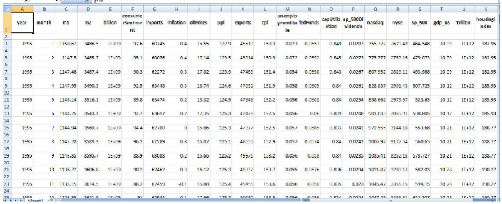
[image:4.595.48.553.350.555.2]company balance sheet, incoming statement, cash flow statement etc. all this data is in semi-structure form all this historical data related to stock can analyse and tries to find a pattern in it.
Figure 1. Input historic data in tabulated form
[image:4.595.132.467.589.780.2] Based on fundamental analysis: - also known as sentimental analysis of stock market. These models explore cyberspace, mostly social media (like twitter) and news, to predict the trends of market.
Gathering all required input data
Here only historical data is used for analysis. Historical data collect from S P 500. The data can be collected according requirement i.e. daily, monthly or yearly. For this Daily stock market data is collected. The data collected from Yahoo finance has many features like open price of stock (Open), close price of stock (Close), Highest price of stock on that day(Highest), Lowest price of stock on that day(Lowest). When correlation is compared between all these variables, it found to be above 0.9 for pairs. Other features like Volume traded (Volume), Adjustment Close (Adj. Close) are having very less correlation with other variables. Features which are highly correlated are considered for analysis. This data is huge size that why required BIG DATA tool. The sources for big data generally fall into one of three categories: Streaming Data, Social Media Data, Publically Available Data.
Analysis of input data
As the input data is historic data, Machine Learning (ML) is used for analysis. Machine learning is a type of artificial intelligence (AI) that provides computers with the ability to learn without being explicitly programmed. Machine learning focuses on the development of computer programs that can teach themselves to grow and change when exposed to new data. Using ML it's possible to quickly and automatically produce models that can analyze bigger, more complex data and deliver faster, more accurate results even on a very large scale.
Prediction process
Predictive analytics is an area of data mining that deals with extracting information from data and using it to predict trends and behaviour patterns. Predictive analytics encompasses a variety of statistical techniques from predictive modelling, machine learning, and data mining that analyze current and historical facts to make predictions about future or unknown events. Regression technique and time series analysis is a form of predictive modelling technique which investigates the relationship between a dependent (target) and independent variable(s) (predictor). This technique is used for forecasting.
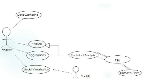
[image:5.595.39.288.637.775.2]Implementation
Figure 3. Use case Diagram
Box Jenkins method
In time series analysis, the Box Jenkins method, named after the statisticians George Box and Gwilym Jenkins, applies autoregressive moving average (ARMA) or autoregressive integrated moving average (ARIMA) models to find the best fit of a time-series model to past values of a time series. Box Jenkins model identification Stationary and seasonality The first step in developing a Box Jenkins model is to determine if the time series is stationary and if there is any significant seasonality that needs to be modelled.
Detecting stationary
Stationary can be accessed from a run sequence plot. The run sequence plot should show constant location and scale. It can also be detected from an autocorrelation plot. Specifically, non-stationary is often indicated by an autocorrelation plot with very slow decay.
Detecting seasonality
Seasonality (or periodicity) can usually be assessed from an autocorrelation plot, a seasonal subseries plot, or a spectral plot.
Differencing to achieve stationary
Box and Jenkins recommend the differencing approach to achieve stationary. However, fitting a curve and subtracting the fitted values from the original data can also be used in the context of Box Jenkins models.
Seasonal differencing
At the model identification stage, the goal is to detect seasonality, if it exists, and to identify the order for the seasonal autoregressive and seasonal moving average terms. For many series, the period is known and a single seasonality term is sufficient. For example, for monthly data one would typically include either a seasonal AR 12 term or a seasonal MA 12 term. For Box Jenkins models, one does not explicitly remove seasonality before fitting the model. Instead, one includes the order of the seasonal terms in the model specification to the ARIMA estimation software. However, it may be helpful to apply a seasonal difference to the data and regenerate the autocorrelation and partial autocorrelation plots. This may help in the model identification of the non-seasonal component of the model. In some cases, the seasonal differencing may remove most or all of the seasonality effect.
Identify p and q
Once stationary and seasonality have been addressed, the next step is to identify the order (i.e. the p and q) of the autoregressive and moving average terms. Different authors have different approaches for identifying p and q. Brockwell and Davis (1991) state "our prime criterion for model selection (among ARMA (p,q) models) will be the AICc", i.e. the Akaike information criterion with correction. Other authors use the autocorrelation plot and the partial autocorrelation plot, described below.
Autocorrelation and partial autocorrelation plots
The sample autocorrelation plot and the sample partial autocorrelation plot are compared to the theoretical behavior of
these plots when the order is known. Specifically, for an AR(1) process, the sample autocorrelation function should have an exponentially decreasing appearance. However, higher-order AR processes are often a mixture of exponentially decreasing and damped sinusoidal components. For higher-order autoregressive processes, the sample autocorrelation needs to be supplemented with a partial autocorrelation plot. The partial autocorrelation of an AR(p) process becomes zero at lag p + 1 and greater, sample partial autocorrelation function is examine to see if there is evidence of a departure from zero. This is usually determined by placing a confidence interval on the sample partial autocorrelation plot (most software programs that generate sample autocorrelation plots also plot this confidence interval).
[image:6.595.83.518.238.495.2]If the software program does not generate the confidence band, it is approximately +- 2/N with N denoting the sample size. The autocorrelation function of a MA (q) process becomes zero at lag q + 1 and greater, sample autocorrelation function is examined to see where it essentially becomes zero. This is done by placing the confidence interval for the sample autocorrelation function on the sample autocorrelation plot. Most software that can generate the autocorrelation plot can also generate this confidence interval. The sample partial autocorrelation function is generally not helpful for identifying the order of the moving average process. The data may follow an ARIMA (p,d,0) model if the ACF and PACF plots of the differenced data show the following patterns:
Figure 4. Decomposition plot S P 500
[image:6.595.79.521.550.782.2] The ACF is exponentially decaying or sinusoidal
There is a significant spike at lag p in PACF, but none
beyond lag p. The data may follow an ARIMA(0,d,q) model if the ACF and PACF plots of the differenced data show the following patterns:
The PACF is exponentially decaying or sinusoidal
There is a significant spike at lag q in ACF, but none
beyond lag q.
In practice, the sample autocorrelation and partial
autocorrelation functions are random variables and do not give the same picture as the theoretical functions. This makes the model identification more difficult. In particular, mixed models can be particularly difficult to identify.
Although experience is helpful, developing good models using these sample plots can involve much trial and error.
Box Jenkins model estimation
[image:7.595.64.549.67.318.2]Estimating the parameters for Box Jenkins models involves numerically approximating the solutions of nonlinear equations. For this reason, it is common to use statistical software designed to handle to the approach fortunately, virtually all modern statistical packages feature this capability. The main approaches to fitting Box Jenkins models are nonlinear least squares and maximum likelihood estimation. Maximum likelihood estimation is generally the preferred technique.
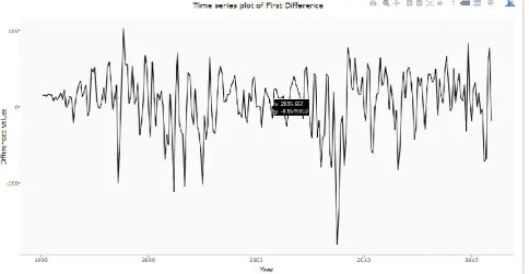
[image:7.595.64.542.362.612.2]Figure 6. Time series plot of first difference of SP 500
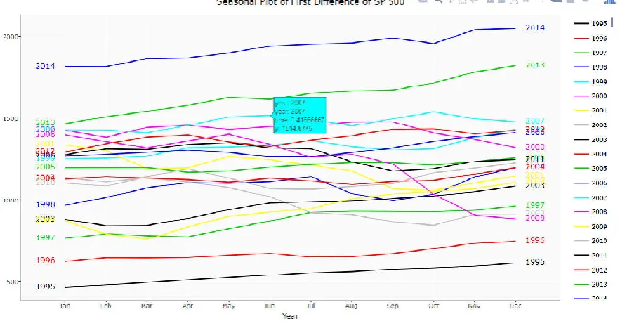
Figure 7. Seasonal plot of first difference of SP 500
Figure 8. Plot of SP 500 ARIMA Model Residuals
Figure 9. Plot 2015 forecast of S P 500
Figure 11. Mean forecast plot of sp 500
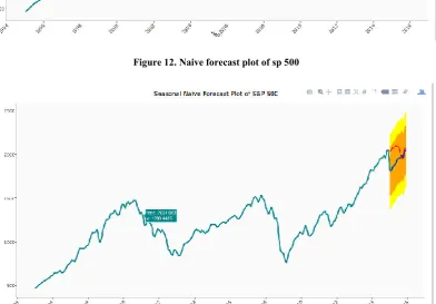
Figure 12. Naive forecast plot of sp 500
Figure 13. Seasonal naive forecast plot of sp 500
[image:9.595.106.499.482.755.2]The likelihood equations for the full Box Jenkins model are complicated and are not included here. See (Brockwell and Davis, 1991) for the mathematical details.
RESULTS
In this research which utilized the time series analysis techniques, time series analysis techniques have outperformed the other techniques in the experiment. Data transformation process opens up another opportunity to be discovered by the targeted algorithms. The use of a different data type by transforming real numbers into categorical ordinal data can improve the outcomes of the techniques. The outcomes are favourable when less structured data are transformed into more structured data in ordinal form. Since there are many other data types, further it can be conducted to compare the effects of transforming various forms of data types in time series analysis techniques used for prediction of stock price trend.
The decomposition of time series is a statistical method that deconstructs a time series into several components
Data- It is the plot of SP500 stock price.
Trend- It reflects the long-term progression of the series
(secular variation). A trend exists when there is an increasing or decreasing direction in the data. The trend component does not have to be linear.
Seasonal- It reflects seasonality (seasonal variation). A
seasonal pattern exists when a time series is influenced by seasonal factors. Seasonality is always of a fixed and known period (e.g., the quarter of the year, the month, or day of the week)
Irregular- It describes random, irregular influences. It
represents the residuals or remainder of the time series after the other components have been removed
[image:10.595.88.521.53.283.2]Seasonal sub-series plots involve the extraction of the seasons from a time series into a subseries. Based on a selected
Figure 14. Exponential smoothing forecast plot of Sp 500
[image:10.595.95.513.337.566.2]periodicity, it is an alternative plot that emphasizes the seasonal patterns is where the data for each season are collected together in separate mini time plots. The Figure 5 is seasonal plot of training set of 1995 to 2014. A time series plot is a graph that can use to evaluate patterns and behaviour in data over time. The graph is plotted time vs. differenced value which gives an illustration of data points at successive time intervals. The seasonal difference of a time series is the series of changes from one season to the next. For monthly data, in which there are 12 periods in a season, the seasonal difference of Y at period t is Yt - Yt-12. Differencing can help stabilize the mean of a time series by removing changes in the level of a time series, and so eliminating trend and seasonality. The figure 7 shows seasonal plot of first order difference of s and p 500. Histogram of the Residuals showing that the deviation is normally distributed. A normal probability plot of the residuals can be used to check whether the variance is normally distributed as well. The figure 8 histogram of SP500 ARIMA model residuals makes the calculation of prediction intervals much easier. Figure 9 graph forecasting 2015 stock market price using historical data from 1995 to 2014. The graph is plotted year with respect to the closing price. In regression analysis, one sometimes carries out a series of Box-Cox transformations of the response variable with a range of values of and, and one then compares the residual sum of squares at these values in order to choose the transformation which gives the best results. Because the residual sum of squares is proportional to the log likelihood, this procedure amounts to approximate maximum likelihood estimation.
The mean model is also the starting point for constructing forecasting models for time series data, including ARIMA model. The blue line is the predicted value of 2015 which is calculated by taking average of training set as per proposed in mathematical model. Estimating technique in which the last period's actual are used as this period's forecast, without adjusting them or attempting to establish causal factors. It is used only for comparison with the forecasts generated by the better (sophisticated) techniques. Here only 2014 value is used to predict 2015 value. In such situations, the forecasting procedure calculates the seasonal index of the season. Exponential smoothing is a rule of thumb technique for smoothing time series data, particularly for recursively applying as many as three low-pass filters with exponential window functions. Figure 14 graph predict the stock value by this method. In statistics, the residual sum of squares (RSS), also known as the sum of squared residuals (SSR) or the sum of squared errors of prediction (SSE), is the sum of the squares of residuals (deviations predicted from actual empirical values of data).
Accuracy
The function accuracy gives multiple measures of accuracy of the model fit: mean error (ME), root mean squared error (RMSE), mean absolute error (MAE), mean percentage error (MPE), mean absolute percentage error (MAPE), mean
absolute scaled error (MASE) and the first-order
autocorrelation coefficient (ACF1). It is decided, based on the accuracy measures, whether to consider this a good fit or not. Error is calculated by following formula generally
Absoulute percent error = (abs(actual value-fitter dor predicted value)/actual value)*100
After calculating using function MAPE=2.142
Conclusion
Using scale-dependent errors as to which model is best for forecasting time series object. Ultimately ARIMA (0,1,1) was the best model at forecasting based on the scale-dependent errors.
Future Scope
This project can be expanded with help of current data which is taken from social media (like twitter, news etc.) to predict the stock trend to view the current best stock in the market.
REFERENCES
"Sentiment Analysis of Stock Market News with Semi-supervised Learning", 2012 IEEE/ACIS 11th International Conference on Computer and Information Science.
Bing Keith, L.I. Chan, C.C. and Carol, O.U. 2014. India, Stock Market Prediction: A Big Data Approach, 2014 IEEE 11th International Conference on e-Business Engineering. Hyndman, Rob J. and George Athanasopoulos "Forecasting:
Principles and Practice" Otexts, May 2012 Web.
Keisuke Mizumoto, Hidekazu Yanagimoto and Michifumi Yoshioka Sentiment Analysis of Stock Market News with
Semi-supervised Learning, 2012 IEEE/ACIS 11th
International Conference on Computer and Information Science.
NIST/SEMATECH e-Handbook of Statistical Methods "Introduction to Time Series Analysis", June, 2016. Peter Zhang, G. 2001. USA "Time series forecasting using a
hybrid ARIMA and neural network model", Received 16 July 1999, Accepted 23 November 2001, Available online 8 January 2002
Schmidt, Drew "Autoplot: Graphical Methods with ggplot2 "Wrathematics, my stack runneth over", June, 2012. Web. Shumway, Robert H. and Stoffer David, S. 2012. "Time Series
Analysis and Its Applications with R Examples", 3rd edition. 2012
Siew, H. L. and Nordin, M. 2012. "Regression techniques for the prediction of stock price trend", in Statistics in Science, Business, and Engineering (ICSSBE), International Conference on Langkawi, University Kuala Lumpur, pp. 1-5, 2012.
Zhen Hu, Jie Zhu and Ken, T.S. 2013. "Stock Market
prediction using Support Vector Machines",6th
International Conference on Information Management, Innovation Management and Industrial Engineering, 2013.
*******