James A. Grant1 2 Alexis Boukouvalas1 Ryan-Rhys Griffiths3 David S. Leslie1 4 Sattar Vakili1 Enrique Munoz de Cote1
Abstract
We consider the problem of adaptively placing sensors along an interval to detect stochastically-generated events. We present a new formulation of the problem as a continuum-armed bandit prob-lem with feedback in the form of partial observa-tions of realisaobserva-tions of an inhomogeneous Pois-son process. We design a solution method by combining Thompson sampling with nonparamet-ric inference via increasingly granular Bayesian histograms and derive anO˜(T2/3)bound on the Bayesian regret inTrounds. This is coupled with the design of an efficent optimisation approach to select actions in polynomial time. In simulations we demonstrate our approach to have substantially lower and less variable regret than competitor al-gorithms.
1. Introduction
In this paper we consider the problem of adaptively placing sensors to detect events occurring stochastically according to a inhomogeneous Poisson process. This is a problem arising in numerous applications including ecology (Heikki-nen & Arjas, 1999), and astronomy (Gregory & Loredo, 1992). Adaptive sequential decision-making that learns an optimal placement of sensors in response to observations can lead to detecting many more events than fixed policies based on an assumed Poisson process rate function. We study the problem under a simple abstract framework which encompasses many possible practical scenarios, including choosing which hours to operate to maximise customer en-gagement, or choosing placement of mobile base stations to service as many requests as possible, as well as the classical
1
PROWLER.io Ltd, Cambridge, United Kingdom2STOR-i Centre for Doctoral Training, Lancaster University, Lancaster, United Kingdom3Department of Physics, University of Cam-bridge, CamCam-bridge, United Kingdom4Department of Mathematics and Statistics, Lancaster University, Lancaster, United Kingdom. Correspondence to: James A. Grant<[email protected]>.
Proceedings of the36th
International Conference on Machine Learning, Long Beach, California, PMLR 97, 2019. Copyright 2019 by the author(s).
sensing applications.
Suppose that a decision-maker is tasked with placing a finite number of sensors along an interval. The decision-maker’s objective is to maximise, through time, a reward function which trades off the number of events detected with the cost of sensing. At each step, each sensor is tasked with sensing a subinterval, with the cost of sensing depending on the length of the subinterval. Only the events that occur in a sensed subinterval are detected. The decision-maker may update the placement of sensors at regular intervals creating a sequential problem where the decision-maker iteratively places sensors and receives feedback on where events occurred.
The decision-maker therefore faces a classic exploration-exploitation dilemma. In each round they will gather in-formation on what was detected in the sensed regions, and will receive a reward. The most informative action is to sense the entire interval, but this may not be the reward-maximising action due to the cost of sensing. Hence the decision-maker must choose sensor placements to trade off learning about regions where information is insufficient, while also capitalising on information they already have to generate large rewards. This paper develops an algorithm to tackle this problem with the aim of minimising Bayesian regret, the difference between the expected reward achieved by constantly selecting an optimal action and the expected reward of actions actually taken, where the expectation is taken with respect to the prior over the reward-generating parameters.
Multi-armed bandits provide models for sequential deci-sion problems, and our problem most closely resembles the continuum-armed or X-armed bandit problem (Agrawal, 1995). In a continuum-armed bandit (CAB) problem a decision-maker sequentially selects points in some d -dimensional continuous space and receives reward in the form of a noisy realisation of some unknown (usually Lips-chitz smooth) function on the space. Our sensor placement problem can map to this framework by considering that the placement of sensors can be represented by the set of end-points of the sensors’ subintervals. Note, however, that the noise and feedback models in the sensor placement prob-lem are more complex than in previous treatments of CAB
models, which have focused on simple numerical reward ob-servations with bounded or sub-Gaussian noise (e.g. Bubeck et al., 2011). In this paper, we handle the added complexities of observing event locations and the heavier-tailed noise of the Poisson distribution.
Our proposed method performs fast Bayesian inference on the rate function, by means of a Bayesian histogram ap-proach (Gugushvili et al., 2018), and makes decisions to trade off exploration and exploitation using Thompson sam-pling (TS) (e.g. Russo et al., 2018). Gugushvili et al.’s ap-proach to nonparametric inference on the continuous action space imposes a mesh structure over the interval, splitting it into a finite number of bins, with the mesh becoming finer as time increases. Inference is then performed over the rate of event occurrence in each bin. TS methods select an ac-tion in a given round according to the posterior probability that it is optimal. In our approach, this is implemented by sampling bin rates from the simple posterior distributions of Gugushvili et al.’s model and selecting an optimal action for these sampled rates via an efficient optimisation algorithm described in Section 3.4.
We analyse the Bayesian regret of the TS algorithm in this setting using similar techniques to those of Russo & Van Roy (2014). This allows us to derive an O˜(T2/3)upper bound on the Bayesian regret that holds across all possible rate functions with a bounded maximum, and has minimal dependency on the prior used by the TS algorithm. The CAB problem with Poisson noise and event data as feedback is to the best of our knowledge unstudied, however our regret upper bound is encouragingly close to theΩ(T2/3)lower bound on simpler CAB models of Kleinberg (2005).
The remainder of the paper is structured as follows. We review related work in Section 2, formalise our model and algorithm in Sections 3, present the regret analysis in tion 4, and conclude with simulation experiments in Sec-tion 5.
1.1. Principal Contributions
The principal contributions of this work are: (i) formulation of a new widely applicable model of sequential sensor place-ment as a CAB; (ii) the first study of CABs with Poisson process feedback, and use of a new progressive discretisa-tion technique as an approximadiscretisa-tion to the continuous acdiscretisa-tion space; (iii) an efficient optimisation routine for sensor place-ment given known event rate; (iv) analysis of the Bayesian regret of a TS approach, resulting in aO˜(T2/3)upper bound; (v) numerical validation of the efficacy of the TS method, and its favourable performance relative to upper confidence bound and-greedy approaches.
2. Related Work
The problem of allocating searchers in a continuous space has been studied by Carlsson et al. (2016) under the assump-tion that the rate of arrivals is known. A first attempt to solve a version of the problem in which the rate must be learned is presented in Grant et al. (2018), in which the space is discretised to a fixed grid for all time. The objective of our paper is to present the first learning version of the problem for the fully continuous space.
The fixed discretisation version of the problem maps directly to Combinatorial Multi-Armed Bandits (CMAB) (Cesa-Bianchi & Lugosi, 2012; Chen et al., 2016). This is a class of problems wherein the decision-maker may pull multiple arms among a discrete set and receives a reward which is a function of observations from individual arms. In the discretised sensor-placement problem, the individual arms correspond to cells of the grid. The model remains relevant for the continuous version of the problem, as by using an increasingly fine mesh, we approximate the problem with a series of increasingly many armed CMABs.
The continuum-armed bandit (CAB) model (Agrawal, 1995) is an infinitely-many armed extension of the classic multi-armed bandit (MAB) problem. There are two main classes of algorithm for CAB problems: discretisation-based ap-proaches which select from a discrete subset of the con-tinuous action space at each iteration, and approaches which make decisions directly on the whole action space. Our proposed method belongs to the former class. Early discretisation-based approaches focused on fixed discretisa-tion (Kleinberg, 2005; Auer et al., 2007), with more recent approaches typically using adaptive discretisations such as a “zooming” approach (Kleinberg et al., 2008) or a tree-based structure (Bubeck et al., 2011; Bull, 2015; Grill et al., 2015) to manage the exploration. Authors who handle the full continuous action space typically use Gaussian process models to capture uncertainty in the unknown continuous function and balance exploration-exploitation in light of this (Srinivas et al., 2009; Chowdhury & Gopalan, 2017; Basu & Ghosh, 2017). As mentioned in Section 1, our problem can map into a CAB, but since our information structure is more complex, our action space has dimension greater than 1, and the stochastic components have heavier tails than usual, standard algorithms and results do not apply.
recently, TS has been studied in the CMAB framework by Wang & Chen (2018) and Huyuk & Tekin (2018) under slightly differing models, but both with bounded reward noise. Both papers demonstrate the asymptotic optimality of TS with respect to the frequentist regret, and we an-ticipate that these results could be extended to univariate exponential families. However, in both of these works, the leading order coefficients can be highly suboptimal. There-fore, rather than attempt to extend these ideas to CABs, we favour an alternative analysis of the Bayesian regret to get bounds that are of slightly suboptimal order but are more meaningful because of their (relatively) small coefficients. The Bayesian regret is less extensively studied than the fre-quentist regret. However the bounds that have been derived for the Bayesian regret of TS (Russo & Van Roy, 2014; Bubeck & Liu, 2013) are powerful as they do not depend on a specific parameterisation of the reward functions.
3. Model and solution
We now formally present our model and solution method.
3.1. Reward and regret
In each of a series of rounds t ∈ N, mt ≥ 0 events
of interest arise at locations Xt,1, ..., Xt,mt ∈ [0,1]
ac-cording to a non-homogeneous Poisson process with rate λ : [0,1]→ R+. U sensors are deployed in each round with each sensor observing a distinct subinterval of[0,1]; the action spaceAconsists of the sets of at mostU disjoint intervals of[0,1]. LetAt⊆[0,1]be the union of the
subin-tervals covered by the sensors in roundt. An eventXt,iis
detected if it lies inAt. The system objective is to maximise
the number of detected events while penalised by a cost of operating the sensors. The expected reward for playing actionAis therefore
r(A) =
Z
A
(λ(x)−C) dx,
whereCis the cost per unit length of sensing. We define the Bayesian regret of an algorithm to be the expected difference (with respect to the prior onλ) between the reward achieved when playing the optimal action in each ofT rounds and the actions taken by the algorithm:
BReg(T) = T
X
t=1
E(r(A∗)−r(At))
whereA∗= arg maxA⊆Ar(A)is the optimal action on the
continuous interval.
3.2. Inference
With the Poisson process rate being defined on the contin-uum[0,1], nonparametric estimation is preferable to a para-metric form. We use the increasingly granular histogram
approach of Gugushvili et al. (2018), since it provides us with fast inference and a concentration rate. At the begin-ning of each roundta piecewise-constant estimation ofλis considered by counting the number of events to have been observed in each ofKtbins. The number of bins will be
gradually increased as rounds proceed. To maintain simplic-ity in the inference and analysis we choose all bins to be of a constant width∆t=Kt−1.
We introduce the notation
Bk,t≡
k−1
Kt
, k Kt
∀ k∈ {1, . . . , Kt}, ∀ t∈N,
to refer to thekth histogram bin at iterationt(the indext is needed to uniquely index a bin since the number of bins changes astincreases). The number of events in binBk,t
in a single observation of the Poisson process is a Poisson random variable with parameterR
Bk,tλ(x) dx. Since this
depends on the width of the bin, we instead estimate the average rate function in a bin, defined as
ψk,t=Kt
Z
Bk,t
λ(x) dx.
We place independent truncated Gamma (TG) priors on each of theψk,tparameters, with shape and scale
parame-tersαandβand support on[0, λmax]whereλmaxis some known upper bound on the maximum of rate functions. (The TG(α, β,0, λmax)distribution has a density proportional to a Gamma(α, β)distribution, but with truncated support
[0, λmax].) In practice theλmaxparameter may be chosen very conservatively; settingλmaxto be too large does not affect the action selection; however it is important to include an upper limit on the prior support to permit tractable regret analysis, and the chosenλmaxappears in the regret bound in Theorem 2.
The consequence of this formulation is that, conditional on actions and observations in the firsttrounds, we have a posterior distribution overλat timetwhich is piecewise constant. Aλtsampled from this posterior takes the form
λt(x) = Kt X
k=1
I{x∈Bk,t}ψ˜k,t, with
˜
ψk,t∼TG(α+Hk,t(t), β+ ∆tNk,t(t),0, λmax), (1)
where Hk,t(s) = Ps
j=1 Pmj
l=1I{Bk,t ⊆ Aj}I{Xj,l ∈
Bk,t}gives the number events observed up to iterations
in binBk,t, andNk,t(s) =P s
j=1I{Bk,t⊆Aj}gives the
number of times to iterationsthat binBk,thas been sensed
(see Section 3.3).
functionλ. In particular,
E(||λt−λ||2)≤t
−2h
2h+1
if Nk,t(t) = t for allk ∈ [Kt]andKt = O(t1/3). We
describe in the next sub-section how the same choice of Ktgives favourable performance in our sequential decision
problem, even when we only observe subintervals of[0,1].
3.3. Thompson sampling
In order to make action selection feasible, and to facilitate the inference using histograms, we constrain the action set of the TS approach using the same (increasingly fine-meshed) grid that the inference is performed over. In particular, in roundt, the actionAtis constrained to lie in the set of
available actionsAt, consisting of those intervals and unions
of intervals where only entire bins (no fractions of bins) are covered and the action consists of at mostU subintervals. RecallU is the number of sensors, and the restriction to at mostU intervals ensures that each sensor can be allocated a single contiguous subinterval. We allow the number of bins Ktto increase at rateO(t1/3)by doubling the number of
bins in line with the growth oft1/3.
Our TS approach is described in Algorithm 1. In each round t, for each bink ∈ {1, . . . , Kt}, a rateψ˜k,t is sampled
according to (1), and then an action is selected that would be optimal if the true rate function were the piecewise-constant combination of these rates. As each bin rate is sampled from the current posterior and the action selected is the optimal action for this set of sampled rates, the selected action is chosen according to the posterior probability that it is the optimal one available. The optimal action conditional on a given sampled rate can be determined efficiently and exactly using the approach described in Section 3.4.
Algorithm 1Thompson Sampling
Inputs:Gamma prior parametersα, β >0, upper trunca-tion pointλmax
Iterative Phase:Fort≥1
• For eachk∈ {1, . . . , Kt}, evaluateHk,t(t−1)and
Nk,t(t−1)and sample an index
˜
ψk,t∼TG(α+Hk,t(t−1), β+∆tNk,t(t−1),0, λmax)
• Choose an actionAt∈ Atthat maximisesr(A)
condi-tional on the true rate being given by the sampledψ˜k,t
values, and observe the events inAt
3.4. Action selection by iterative merging (AS-IM)
In this section we describe a routine, called action selection by iterative merging (AS-IM), for efficiently determining the optimal action conditional on a given sampled rate func-tion. For the piecewise constantλtfunctions sampled by
the TS approach, the above optimization problem can be formulated as an integer program in which each binBk,tis
either searched or not. Grant et al. (2018) solve this program (albeit for more general cost functions and fixed discretisa-tion) using traditional integer programming methods, with exponentially high computation complexities inKtandU.
We instead introduce an efficient optimal action selection policy with polynomial sample complexity.
Firstly, we introduce additional notation that will be useful for explaining the algorithm. Throughout this section we takeλas fixed and piecewise constant on binsBk,t, and
provide a method to findA∗for thisλ. An actionA∈ Acan be written as the union of disjoint intervals: A=∪U
u=1Iu
andIu∩Iu0 =∅for all1≤u, u0≤U. Define theweight of an intervalI∈[0,1]asw(I) =R
I(λ(x)−C)dx. Thus,
we may write the optimal action as
A∗= argmax
{Iu}Uu=1
U
X
u=1 w(Iu).
AS-IM creates an initial set of candidate intervalsI =
{In}Nn=1such that eachInis the union of a number of
ad-jacentBk,t, and fork= 2, ..., Kt,Bk,tandBk−1,tbelong
to the sameInif and only ifw(Bk,t)andw(Bk−1,t)have the same sign. Notice that, by construction, the weights of adjacent intervals have opposite signs. If the number of intervals in I with positive weight is not bigger than U, AS-IM returns all such intervals as the optimal action. Otherwise, AS-IM proceeds to the next step.
AS-IM iteratively reduces the number of intervals with posi-tive weights by merging the intervals. Specifically, letM =
{n∈ {2, . . . , N −1} : |w(In)| ≤ |w(In−1)|,|w(In)| ≤
|w(In+1)|}be the set of intervals that should be considered for merging. If M is empty, no further merging should take place. IfM is nonempty letn= argminM|w(In)|be the label inM with the smallest absolute weight; AS-IM mergesInwith its two neighbour intervalsIn+1andIn−1 into one interval and updates the set of intervalsI. The merging procedure repeats until eitherM is empty or the number of intervals with positive weight equalsU. At this point AS-IM returns theUintervals with the largest weights asI1∗, I2∗, ..., IU∗.
We have the following result on AS-IM guaranteeing its optimality and efficiency. The proof is given in the supple-mentary material via an induction argument.
4. Regret Bound
In this section, we present our main theoretical contribution: an upper bound on the Bayesian regret of the TS approach. There is an inevitable minimum contribution to regret due to the optimal action likely not being in our discretised action set. But by allowing the mesh to become more fine as more observations are made, we will gradually reduce this discretisation regret and permit a closer approximation to the true underlying rate function.
For the analysis that follows it will be useful to defineA∗t = arg maxA∈Atr(A)as the optimal action available in round t. We then define for anyA∈ Atandt∈N:
δ(A) =r(A∗)−r(A)
δt(A) =r(A∗t)−r(A)
as thesingle-round regretof the actionAwith respect to the optimal continuous action and the optimal action available to the algorithm in roundtrespectively. The difference be-tweenδ(A)andδt(A)is that the “discretisation regret” by
choosing actions only fromAtis present only inδ(A).
Min-imising the true regretδ(A)requires balancing out estima-tion accuracy (requiring a coarse grid) versus discretisaestima-tion regret (requiring a finer grid). We find below that choosing the number of binsKtto be orderO(t1/3)provides the best
theoretical performance guarantees. This coincides with the optimal posterior contraction rate findings in Gugushvili et al. (2018). We verify this numerically in Section 5 and find that this rebinning rate is superior to a faster linear rate of rebinning.
Theorem 2. Consider the setup of Section 3, withU sen-sors, and cost of sensing C. Suppose we choose Kt
such that there exist positive constants K, K such that
Kt1/3 ≤ Kt ≤ Kt1/3. Then the Bayesian regret of
Al-gorithm 1 satisfies
BReg(T)≤4K log(T+ 1) log(T) + 2λmax
T1/3
+ CU K−1+
q
24Kλmaxlog(T)T2/3.
This main result is that we have aO(T2/3log1/2(T))bound on the Bayesian regret. A lower bound for the problem is not currently available. The closest result available is that of Kleinberg (2005) for CABs with bounded Lipschitz smooth reward function and bounded noise. The bound holds only for a one-dimensional action space and is of orderΩ(T2/3). The material differences in our setting are that the obser-vation noise is unbounded (with Poisson tails), our reward function is defined on higher dimension (the unrestricted action space of the underlying CAB is of dimension2U), and that we observe additional information in the form of event locations. In the context of the nearest related results therefore, Theorem 2 suggests that the TS approach is a strongly performing policy.
Proof of Theorem 2. The Bayesian regret can be decom-posed as the sum of the regret due to discretisation and the regret due to selecting suboptimal actions inAt, as follows
BReg(T) =E
T
X
t=1 δ(A∗t)
+E
T
X
t=1 δt(At)
The expectation in the first term only averages overλ func-tions, not over action selection, and the sum can be upper bounded uniformly over allλ’s by considering the rate of re-binning. In particular we have the following lemma, proved in the supplementary material.
Lemma 1. The regret due to discretisation is bounded by
T
X
t=1
δ(A∗t)≤CU K−1T2/3,
uniformly over all ratesλ.
To handle the stochastic part of the regret we use a decompo-sition from Propodecompo-sition 1 of Russo & Van Roy (2014). For allT, for all1≤t≤Tand for allA∈ At, letLt,T(A)and
Ut,T(A)satisfy−C|A| ≤Lt,T(A)≤Ut,T(A)(see below
for a judicious choice of these variables). Then, for anyT,
E
" T
X
t=1 δt(At)
#
=E
" T
X
t=1
r(A∗t)−r(At)
#
=E
" T
X
t=1
Ut,T(At)−r(At)
#
+E
" T
X
t=1
r(A∗t)−Ut,T(A∗t)
#
≤E
" T
X
t=1
Ut,T(At)−Lt,T(At)
#
+λmax×
" T X
t=1
P(r(A∗t)> Ut,T(A∗t)) + T
X
t=1
P(r(At)< Lt,T(At))
#
The key step here is the second equality, which holds for TS because the distribution ofUt(At)is precisely the
distribu-tion ofUt(A∗t)due to the method of selectingAt. The final
step follows by noting that, for anyA,
E[r(A)−Ut,T(A)]
≤E(r(A)−Ut,T(A))I{r(A)−Ut,T(A)>0}
≤λmaxP(r(A)> Ut,T(A)),
and similarly forE[Lt,T(A)−rt(A)]. Theλmaxterm arises fromr(A)≤λmax−C|A|andUt,T(A)≥ −C|A|for all
A∈ At.
We will chooseLt,T andUt,T so that each sum converges.
(2018) for Poisson random variables inspire the definition of
Dk,T(t−1) =
2 log(t) ∆TNk,T(t−1)
+
s
6λmaxlog(t)
∆TNk,T(t−1)
for allk∈[KT], with upper and lower confidence bounds
on the reward of an actionA∈ Atat timet∈Nas follows:
Ut,T(A) = ∆T
X
k:Bk,T⊆A ˆ
ψk,T(t−1) +Dk,T(t−1)−C|A|,
Lt,T(A) = ∆T
X
k:Bk,T⊆A ˆ
ψk,T(t−1)−Dk,T(t−1)−C|A|,
whereψˆk,T(t) =
Hk,T(t)
∆TNk,T(t) gives the empirical mean in
binBk,T aftertrounds. It is in the definition ofUt,T and
Lt,T that we see the need for aT-dependence in our choice
of upper and lower confidence bounds—we need to count the number times actionsAtfort < T selected the bin
Bk,T defined for timeT.
In the supplementary material we prove the following lem-mas, which when combined are sufficient to complete the proof of Theorem 2.
Lemma 2. ForUt,T andLt,T as defined above, we have
T
X
t=1
Ut,T(At)−Lt,T(At)≤
4Klog(T) log(T+ 1)T1/3+
q
24Kλmaxlog(T)T2/3
Lemma 3. The deviation probabilities can be bounded
P
r(At)∈/ [Lt,T(At), Ut,T(At)]
≤2KTt−2
Combining these results we have:
BReg(T)≤CU K−1T2/3+ 4Klog(T) log(T+ 1)T1/3
+
q
24Kλmaxlog(T)T2/3+ 2KTλmax
T
X
t=1
2t−2
which gives the required result asP∞
t=1t− 2≤ π2
6.
5. Simulations
In this section, we provide simulation examples on the per-formance of the Thompson sampling approach presented in Section 3.3. We first examine the effect of the rebin-ning rate on the regret and then investigate the performance of the Thompson sampling approach in relation to other algorithms.
0 200 400 600 800 1000
timestep 0
1000 2000 3000 4000 5000
Cumulative regret
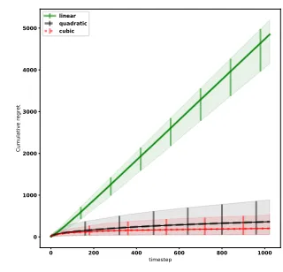
[image:6.612.336.496.83.237.2]linear quadratic cubic
Figure 1.Cumulative regret comparing different rebinning rates.
5.1. Effect of rebinning rate
Firstly we examine the effect of different rebinning rates in a simple unimodal setting withλ(x) =1000
21 (x−x
2),C= 10,
and U = 1 sensor. This setting is chosen such that the optimal action can be calculated asA∗ = [0.3,0.7]. Here, and throughout our experiments, we set the prior parameters for Thompson sampling to beα = 0.5 andβ = 0.5/C, where scaling by costC makes the prior relevant to the expected scale of costs in the problem. We also set the truncationλmaxto be ten times the true maximal value of λ;λmaxis an inconvenient parameter that is only needed for the theory, so we set it to a conservative large value that should have no influence on the real behaviour of the algorithm. The experiment is run 10 times forT = 1024
timesteps starting withK0= 4bins.
We compare linear, square root and cube root rebinning rates: the number of binsKtis doubled in rounds wheret
(in the linear case),t1/2(square root case) ort1/3(cube root case) is twice its value at the last rebinning time. Actions are selected using the TS method of Algorithm 1 and Fig. 1 shows that the cumulative regret is consistently lower under the cube root rate. While under the linear rebinning rate, ac-tions with reward close to that ofA∗become available more quickly, reducing the discretisation regret, the issue is that the majority of bins contain very little data and the posterior inference is heavily dependent on the prior. Under the cube root (and indeed square root) rebinning rate the action set grows more slowly but the unavoidable discretisation regret is balanced by better action selection. The square root case is surprisingly similar to the cube root case despite a weaker theoretical rate in this case. We demonstrate the shrinking of the discretisation regret in the supplementary material.
of the experiment. The posterior under the linear rebinning is highly unconcentrated with simply insufficient numbers of observations in almost all bins. The cube root rate on the other hand results in a posterior which is much more concentrated about the truth in the region where it matters.
(a) Linear
[image:7.612.103.241.160.493.2](b) Cube Root
Figure 2.Posterior under the linear and cube root rebinning rates at roundT= 1024. We show the true rate function (blue) and cost (pink), the posterior credible interval (light green) and mean (dark green) per bin. Thompson samples are shown in black, and the selected interval,AT, is the (red) vertical bar. The initial number
of bins is 4 in both cases and the final number of bins,KT, is
2048 for the linear rebinning schedule and 32 bins for the cube root schedule.
5.2. Comparison to Baselines
We now compare different baseline policies solely using the cube root rebinning schedule. Experiments with the unimodal rate of Section 5.1 were not informative since the problem is an easy one. We instead use a bimodal rate λ(x) = max 0.001,√15 sin(10x)
(10x+1)+x
withC= 2andU = 2
sensors. Each experiment was run 10 times forT = 1000
time steps, starting with K0 = 16 bins and terminating withKT = 128bins. In addition to the Thompson
sam-pling approach described in Section 3.3, we consider three other algorithms, which are summarised here and described precisely in the supplementary material. (i) An upper confi-dence bound (UCB) approach, in which the decision-maker chooses what would be an optimal action if the true rates wereUt,t (as defined in the proof of Theorem 1); this is
essentially the FP-CUCB algorithm of Grant et al. (2018), albeit with a changing mesh, and requires the specification of an upper boundλmaxon the rate in order to define the action selection. In our experiments we fix thisλmaxto the correct value; in practise a conservative estimate is usually available, but for this algorithm the choice ofλmaxstrongly affects the actions selected, in contrast with the TS algo-rithm, and we choose the most favourableλmax for this algorithm. (ii) A modified-UCB approach (mUCB) where the empirical mean for each histogram binψˆk is used in
place of the overall maximum rateλmax. Note this modi-fication invalidates the concentration results used in Grant et al. (2018), but appears to improve performance in prac-tice. (iii) An -Greedy approach where the intervals are selected according to the empirical mean for each binψˆk
but occasionally an explorative randomisation step occurs in which the algorithm samples, for each bin, a draw from the prior. The randomisation step is taken with probability = 0.01.
0 200 400 600 800 1000
timestep 0
500 1000 1500 2000 2500 3000 3500
Cumulative regret
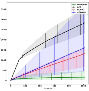
Thompson UCB mUCB
ε-Greedy
Figure 3.Cumulative regret plot for the bimodal rate functions. The experiments are repeated 10 times and the mean and 95% empirical confidence interval is shown for each policy.
[image:7.612.347.495.417.567.2]true rate is low and there is little uncertainty. In contrast the modified-UCB values, that do not depend onλmax, are less inflated where the uncertainty is low (Figure 4(c)) resulting in more often choosing a better action. In Fig. 3 the-Greedy achieves similar mean regret to modified-UCB but with a higher variance. The-Greedy approach has the highest variance due to the greediness of the algorithm. A higher value ofwould reduce variance but would increase the exploration cost. The TS approach consistently outperforms all other policies.
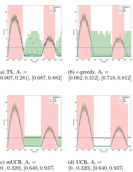
Further intuition can also be gained from the posterior ex-amples shown in Figure 4. These were selected at time stepT = 900from one of the experimental runs. The TS approach has selected an action close to optimal. Further, the posterior variance outside the optimal interval is signif-icantly higher that in the selected regions as only a small number of observations were taken in those regions demon-strating the high efficiency of the method. In contrast both UCB approaches have uniformly low posterior variance in the entirety of the domain reflecting the large number of observations taken incurring a high exploration cost. In contrast, the-Greedy approach selects smaller than optimal intervals with high posterior variance outside these regions. This reflects an under-exploration of the greedy approach which is only able to escape bad local minima when the randomisation step is used.
In summary, the TS approach outperforms all the other approaches we have considered and is able to efficiently trade-off exploration penalty and exploitation reward.
6. Conclusion
We have presented a continuum-armed bandit model of sequential sensor placement. This model introduces the complexities of point process data and heavy-tailed reward distributions to continuum-armed bandits for the first time through its Poisson process observations. We proposed a Thompson sampling approach to make decisions based on fast non-parametric Bayesian inference and an increasingly granular action set, and derived an upper bound on the Bayesian regret of the policy which is independent of the choice of prior distribution.
In our simulation study we have studied two aspects of our approach. Firstly we examined the effect of the rebinning rate on posterior inference and regret. The theoretically-optimal cube root rate resulted in more accurate posterior inference than a linear or square root rebinning rate. This effect was also evident in a lower regret for the cube root rate.
Our empirical study also contrasted our Thompson sampling approach to alternative approaches like UCB or-greedy policies. In both the cases we examined, we found the other
(a) TS,At=
[0.007,0.281],[0.687,0.882]
(b)-greedy,At=
[0.062,0.312],[0.718,0.812]
(c) mUCB,At= [0.,0.320],[0.640,0.937]
(d) UCB,At=
[image:8.612.312.536.77.367.2][0.,0.320],[0.640,0.937]
Figure 4.Posterior under different action selection strategies for the bimodal test function. The true rate function (orange), pos-terior mean (blue) and 95% confidence interval (green infill) is shown. Rate samples for each method are shown in black for each bin and the cost threshold is the (magenta) horizon-tal dashed line. The optimal action is to select two intervals
A∗= [0.013,0.280],[0.675,0.882].
methods either over-explored (e.g. UCB) or over-exploited (e.g.-greedy). The TS approach achieved the best trade-off between the two and consistently achieved the lowest regret.
The observation model and rebinning strategies we have presented here are straightforward; it would be interesting to extend the algorithm and analysis to account for imper-fect observations and to allow for heterogeneous bin widths, letting us capture more detail of the rate function in ar-eas where we have made many observations and adopt a smoother estimate in others.
References
Agrawal, R. The continuum-armed bandit problem. SIAM Journal on Control and Optimization, 33:1926–1951, 1995.
Agrawal, S. and Goyal, N. Analysis of Thompson Sampling for the multi-armed bandit problem. InCOLT, 2012.
Auer, P., Ortner, R., and Szepesv´ari, C. Improved rates for the stochastic continuum-armed bandit problem. In
COLT, pp. 454–468, 2007.
Basu, K. and Ghosh, S. Analysis of Thompson sampling for Gaussian process optimization in the bandit setting, 2017. arXiv:1705.06808.
Bubeck, S. and Liu, C. Prior-free and prior-dependent regret bounds for thompson sampling. InNeurIPS, pp. 638–646, 2013.
Bubeck, S., Munos, R., Stoltz, G., and Szepesv´ari, C. X -armed bandits. J. Mach. Learn. Res., 12:1655–1695, 2011.
Bull, A. Adaptive-treed bandits. Bernoulli, 21:2289–2307, 2015.
Carlsson, J., Carlsson, E., and Devulapalli, R. Shadow prices in territory division. Netw. Spat. Econ., 16:893– 931, 2016.
Cesa-Bianchi, N. and Lugosi, G. Combinatorial bandits. J. Comput. Syst. Sci., 78:1404–1422, 2012.
Chen, W., Wang, Y., Yuan, Y., and Wang, Q. Combinatorial multi-armed bandit and its extension to probabilistically triggered arms. J. Mach. Learn. Res., 17:1746–1778, 2016.
Chowdhury, S. and Gopalan, A. On kernelized multi-armed bandits, 2017. arXiv:1704.00445.
Grant, J., Leslie, D., Glazebrook, K., Szechtman, R., and Letchford, A. Adaptive policies for perimeter surveillance problems, 2018. arXiv:1810.02176.
Gregory, P. and Loredo, T. A new method for the detec-tion of a periodic signal of unknown shape and period.
Astrophys. J., 398:146–168, 1992.
Grill, J., Valko, M., and Munos, R. Black-box optimization of noisy functions with unknown smoothness. InNeurIPS, pp. 667–675, 2015.
Gugushvili, S., van der Meulen, F., Schauer, M., and Spreij, P. Fast and scalable non-parametric bayesian inference for poisson point processes, 2018. arxiv:1804.03616.
Heikkinen, J. and Arjas, E. Modeling a Poisson forest in variable elevations: a nonparametric bayesian approach.
Biometrics, 55:738–745, 1999.
Huyuk, A. and Tekin, C. Thompson sampling for combina-torial multi-armed bandit with probabilistically triggered arms, 2018. arXiv:1809.02707.
John, S. T. and Hensman, J. Large-scale Cox pro-cess inference using variational Fourier features, 2018. arXiv:1804.01016.
Kaufmann, E., Korda, N., and Munos, R. Thompson sam-pling: An asymptotically optimal finite-time analysis. In
ALT, pp. 199–213, 2012.
Kirichenko, A. and Van Zanten, J. Optimality of poisson process intensity learning with gaussian processes. J. Mach. Learn. Res., 16:2909–2919, 2015.
Kleinberg, R. Nearly tight bounds for the continuum-armed bandit problem. InNeurIPS, pp. 697–704, 2005.
Kleinberg, R., Slivkins, A., and Upfal, E. Multi-armed bandits in metric spaces. InProc. 40th Annu. ACM Symp. on Theory of Computing, pp. 681–690, 2008.
Komiyama, J., Honda, J., and Nakagawa, H. Optimal regret analysis of Thompson sampling in stochastic multi-armed bandit problem with multiple plays, 2015. arXiv:1506.00779.
Korda, N., Kaufmann, E., and Munos, R. Thompson sam-pling for 1-dimensional exponential family bandits. In
NeurIPS, pp. 1448–1456, 2013.
Luedtke, A., Kaufmann, E., and Chambaz, A. Asymptoti-cally optimal algorithms for multiple play bandits with partial feedback, 2016. arXiv:1606.09388v1.
May, B., Korda, N., Lee, A., and Leslie, D. Optimistic Bayesian sampling in contextual-bandit problems. J. Mach. Learn. Res., 13:2069–2106, 2012.
Russo, D. and Van Roy, B. Learning to optimize via poste-rior sampling.Math. Oper. Res., 39:1221–1243, 2014.
Russo, D. J., Van Roy, B., Kazerouni, A., Osband, I., and Wen, Z. A tutorial on Thompson sampling.Found. Trends Mach. Learn., 11:1–96, 2018.
Srinivas, N., Krause, A., Kakade, S. M., and Seeger, M. Gaussian process optimization in the bandit setting: No regret and experimental design, 2009. arXiv:0912.3995.
Thompson, W. On the likelihood that one unknown prob-ability exceeds another in view of the evidence of two samples.Biometrika, 25:285–294, 1933.
A. Regret bound proofs
PROOF OFLEMMA1DefineAmin,t=TA∈At:A∗⊆AAas the smallest interval (or union of intervals) inAtcontaining the optimal interval (or
union of intervals). It will be easier to bound the regret ofAmin,tthanA∗t wrtA∗. We have, fort∈N,
δ(A∗t) =r(A∗)−r(A∗t)
≤r(A∗)−r(Amin,t)
=
Z
A∗
(λ(x)−C) dx−
Z
Amin,t
(λ(x)−C) dx
=C|Amin,t\A∗| −
Z
Amin,t\A∗ λ(x)dx
≤2CU∆t.
Here, the final inequality holds since2∆tbounds the difference between the lengths of subintervals ofAmin,tandA∗t, and
there areUsuch subintervals. Since∆t=Kt−1≤K
−1T−1/3the result follows immediately.
PROOF OFLEMMA2
Consider the term inside the expectation
T
X
t=1
Ut,T(At)−Lt,T(At) = 2∆T T
X
t=1 X
k:Bk,T⊆At
Dk,T(t−1)
= 2∆T T
X
t=1 X
k:Bk,T⊆At
2 log(t) ∆TNk,T(t−1)
+
s
6λmaxlog(t)
∆TNk,T(t−1)
= 2∆T T
X
t=1
KT X
k=1
I{Bk,T ⊆At}
2 log(t)
∆TPt−1
s=1I{Bk,T ⊆As} +
s
6λmaxlog(t)
∆TPt−1
s=1I{Bk,T ⊆As}
≤2∆T KT X
k=1
Nk,T X
j=1
2 log(T)
j∆T +
s
6λmaxlog(T) j∆T
≤2∆TKT
T
X
j=1
2 log(T)
j∆T +
T
X
j=1 s
6λmaxlog(T) j∆T
= 4KTlog(T) log(T+ 1) +
p
24λmaxKTlog(T)T1/2
≤4Klog(T) log(T+ 1)T1/3+
q
24Kλmaxlog(T)T2/3
PROOF OFLEMMA3
We have the following, which holds for any roundt
P
r(At)∈/ [Lt,T(At), Ut,T(At)]
≤P
r(At)≤Lt,T(At)
+P
r(At)≥Ut,T(At)
=P
X
k:Bk,T⊆At ψk,T ≤
X
k:Bk,T⊆At h
ˆ
ψk,T(t−1)−Dk,T(t−1)
i
+P
X
k:Bk,T⊆At ψk,T ≥
X
k:Bk,T⊆At h
ˆ
ψk,T(t−1) +Dk,T(t−1)
i
≤ X
k:Bk,T⊆At "
P
ψk,T−ψˆk,T(t−1)≤ −Dk,T(t−1)
+P
ψk,T −ψˆk,T(t−1)≥Dk,T(t−1)
#
≤
KT X
k=1 P
|ψk,T −ψˆk,T(t−1)| ≥
2 log(t) ∆TNk,T(t−1)
+
s
6λmaxlog(t)
∆TNk,T(t−1)
≤
KT X
k=1
t−1 X
s=1 P
|ψk,T −ψˆk,T(t−1)| ≥
2 log(t) ∆TNk,T(t−1)
+
s
6λmaxlog(t)
∆TNk,T(t−1)
Nk,T(t−1) =s
≤2KTt−2.
The final inequality is a direct application of Lemma 1 of (Grant et al., 2018) which in turn exploits Bernstein’s Inequality for independent Poisson random variables.
B. Proof of optimality and efficiency of AS-IM
PROOF OFTHEOREM1Recall that the reward of an action is the sum of the weights of the intervals that comprise that action.
We prove the theorem by induction. Assume at least one initialInhas a positive weight (otherwise the optimal action is to
do no sensing). ForN = 1initial interval, which therefore has a positive weight, AS-IM simply returns this interval, which is optimal. ForN = 2initial intervals, with one positive weight, AS-IM returns the postitively-weighted interval, which is the optimal action. Now, assuming AS-IM returns the optimal action forN≥1, we prove that AS-IM returns the optimal action forN+ 2initial intervals. The result follows by induction.
GivenI ={In}Nn=1+2, if the number of intervals inI with positive weight is not bigger thanU, AS-IM returns all such intervals. This is the optimal action since all bins with positive reward can be covered without incurring the cost of any bins with negative reward; any other action either omits a positive-reward bin, or includes a negative-reward bin.
Similarly, consider the situation in which no interval satisfies the merging condition. Suppose that the optimal actionA∗
places a sensor on a sequence of intervalsIm∪ · · · ∪Inwithn > m. Clearly we must havew(Im)>0andw(In)>0since
otherwise the total weight could be increased by omitting the negatively-weighted end interval. But the fact that no interval can be merged implies that either|w(Im+1)|>|w(Im)|or|w(In−1)|>|w(In)|. Hence removing eitherIm∪Im+1or In−1∪In from the sensor will improve the total weight. It follows that, underA∗, each sensor is allocated to a single
interval, and allocating to theU highest-weight intervals, as specified by AS-IM, maximises the reward.
Now, assume that at least one interval is merged in AS-IM. LetInbe the interval which minimises|w(In)|and so is the first
interval which is merged with its neighbours in AS-IM into a single intervalI˜n =In−1∪In∪In+1. LetA˜∗be AS-IM’s
solution for the set of intervalsI˜={I1,· · ·, In−2,I˜n, In+2,· · · , IN+2}. By induction,A˜∗is optimal forI˜. We prove that A∗, the optimal solution forI, is equal toA˜∗. To prove this, we consider different cases based on the sign ofw(In).
Case 1:w(In)<0. First note that the optimal solution cannot include only one neighbour ofIn. IfIn−1were included butIn+1were not, we could add bothInandIn+1and increase the overall weight (sinceIn has the smallest absolute
sensor in place of the two that coverIn−1andIn+1, addingIntoA∗, and (ii) redeploying the sensor we have saved to either
split one existing sensor by removing a negative-weightImwith|w(Im)|>|w(In)|, or adding a new positive-weightIm
with|w(Im)|>|w(In)|. The net outcome is an improved total weight. We have shown thatA∗includes either all or none
ofIn−1∪In∪In+1. SinceA∗is optimal forI, and the restriction toI˜does not prevent AS-IM from finding this optimal
A∗, it follows thatA˜∗=A∗.
Case 2:w(In)>0. Under the optimal solutionA∗, a sensor cannot have a negative-weighted interval as an end interval, since dropping the negative-weight interval only increases the total weight. Furthermore, a sensor cannot includeInas
an end interval of a series of intervals, since then the total weight could be improved by stopping sensing bothInand its
sensed neighbour. Thus ifInis included inA∗then either a sensor is observing onlyIn, or a single sensor observes all of
In−2∪In−1∪In∪In+1∪In+2. As in Case 1, if a sensor is observing onlyInwe can improve onA∗by redeploying this
sensor to either sense a better interval, or stop sensing an interval which has a higher negative weight than is lost by stopping sensingIn. So again, underA∗,Inis either sensed with all its neighbours, or none of them are sensed. The same logic as in
Case 1 ensuresA˜∗=A∗.
Complexity: AS-IM requires sorting theN initial intervals. Noticing that there are at mostN mergings, and assuming constant complexity for each merging, AS-IM offers anO(NlogN)sample complexity. SinceN ≤Kt, AS-IM has a
sample complexity not bigger thanO(KtlogKt).
C. Discretisation error under linear and cubic root rates
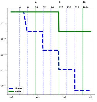
[image:12.612.213.380.387.563.2]The effect of the different rates on the unavoidable discretisation error is depicted in Figure 5. The regret for the linear rate is reduced at a faster rate than for the cubic root rate as the number of bins is increased at a much faster rate. However as we show in the main paper (Section 5.1) the other part of the regret due to error in action selection from the model forecast is much higher under the linear regret rate.
Figure 5.Instantaneous regret comparing linear and cube root rebinning rates. The vertical lines depict the rebinning times for the two different rate schedules. The time step (horizontal axis) and the regret (vertical axis) are both on a log scale. The number of bins for each rebinning rate are shown on the top horizontal axis.
D. Baselines used in the empirical study
In the paper we have compared the TS approach other approaches which we now describe in more details.
Algorithm 2UCB
Inputs:Upper boundλmax≥maxx∈[0,1]λ(x) Initialisation Phase:Fort= 1
• SelectA= [0,1]
Iterative Phase:Fort≥2
• For eachk∈ {1, . . . , Kt}, evaluateHk,t(t−1)andNk,t(t−1)and calculate an index
¯
ψk,t=
Hk,t(t−1) ∆tNk,t(t−1)+
2 log(t) ∆tNk,t(t−1) +
s
6λmaxlog(t)
∆tNk,t(t−1).
• Choose an actionAtthat maximisesr(A)conditional on the true rate being given by theψ¯k,tvalues
• Observe the events inAt
2. A modified-UCB approach (mUCB) which has the same form as Algorithm 1 exceptλmaxis replaced with the empirical mean. Note this modification breaks the upper bound regret guarantee. The indices are :
¯
ψk,t= ˆψk,t(t−1) +
2 log(t) ∆tNk,t(t−1)+
s
6 ˆψk,t(t−1) log(t)
∆tNk,t(t−1) , k∈[Kt]
whereψˆk,t(t−1) =
Hk,t(t−1)
∆tNk,t(t−1).
3. An-Greedyapproach where with probability1−pan actionAtis selected that maximisesr(A)conditional on the
rate being given by the empirical mean valuesψˆk,t. With probabilityp, the action is instead chosen by sampling rates ˜