ISSN Online: 2169-9631 ISSN Print: 2169-9623
DOI: 10.4236/ojer.2018.72009 May 31, 2018 141 Open Journal of Earthquake Research
The High Frequency Decay Parameter
κ
(Kappa)
in the Region of North East India
Renu Yadav
1, Dinesh Kumar
1, Sumer Chopra
21Department of Geophysics, Kurukshetra University, Kurukshetra, Haryana, India
2Institute of Seismological Research, Gandhinagar, Gujarat, India
Abstract
The high frequency decay parameter
κ
has been considered as one of the
im-portant parameters required in the simulation of earthquake strong ground
motions necessary for the proper evaluation of seismic hazard of a region. The
present study estimated “
κ
” for the highly seismic active region of North East
India. The spectral analysis of 598 accelerograms of 32 earthquakes has been
done using
[1]
approach for this purpose. The average values of “
κ
” have been
found to be 0.049, 0.047 and 0.040 for L-, T- and V-component respectively.
The distance dependence of
κ
is not significant in the region. The
κ
0 (κ
at R =
0) for soft rock stations is found to be more than those of hard rock sites in
consistent with other similar studies. The correlation between “
κ
” and
earth-quake magnitude at most of the stations for the region under study is not
sig-nificant which indicates that
κ
depends on the site conditions in the region.
The
κ
values estimated in the present study are useful for the evaluation of
seismic hazard of the region.
Keywords
Kappa, GMPE, Strong Ground Motion, Simulation, Seismic Hazard
1. Introduction
The spectral shape of earthquake strong ground motions plays an important role
in the simulation of realistic accelerograms using different techniques. The
si-mulated accelerograms are crucial for the proper evaluation of seismic hazard of
a region. Different factors including attenuation, velocity and site conditions etc.
control the spectral characteristics of the strong ground motions. It has been
suggested that the spectrum of strong ground motion from earthquakes is flat
above the corner frequency
[2]
to the maximum frequency (
f
max) after which the How to cite this paper: Yadav, R., Kumar,D. and Chopra, S. (2018) The High Fre-quency Decay Parameter κ (Kappa) in the Region of North East India. Open Journal of Earthquake Research, 7, 141-159. https://doi.org/10.4236/ojer.2018.72009
Received: April 26, 2018 Accepted: May 28, 2018 Published: May 31, 2018
Copyright © 2018 by authors and Scientific Research Publishing Inc. This work is licensed under the Creative Commons Attribution International License (CC BY 4.0).
DOI: 10.4236/ojer.2018.72009 142 Open Journal of Earthquake Research
spectrum decays fast
[3]
. This phenomenon of high-frequency band limitation
of radiated earthquake energy has been given the name “the crashing spectrum
syndrome” by
[4]
and attributed this primarily to the local site effects.
[5]
sug-gested the source (fault nonelasticity) as cause for “
f
max” not the site.[6]
de-scribed a site attenuation parameter “
t
*” in the form of exponential decay term
e
−πft*to the spectral attenuation of the waves.
[1]
introduced a spectral decay parameter—
κ
(Kappa) to model the high
fre-quency spectral attenuation. They defined the parameter “
κ
” as:
0
e
f;
EA
f
f
A
=
−π>
(1)
where
A
0 depends on the source, epicentral distance and other factors,f
E is thefrequency above which the spectral amplitude follows an exponential decay. The
studies have been done to attribute the origin of “
κ
” to source, site and/or path
attenuation.
[7]
and
[8]
have suggested that “
κ
” represents the near surface as
well as propagation path attenuation. Some studies suggest that “
κ
” is source
re-lated
[9]
[10]
[11]
[12]
.
[13]
assumes “
κ
” as a parameter related either to source
or site effects. It is considered as site parameter by
[14]
[15]
found that “
κ
” was
independent of earthquake size within magnitude range M < 3.5 for the events
occurred in the region of Northeastern Sonora, Mexico.
[16]
also found no
cor-relation between “
κ
” and magnitude.
In spite of the lack of agreement on the physical origin of “
κ
”, it has been
widely used in number of seismological applications like computation of site
amplification factors, ground motion prediction equations
[17]
[18]
. It has
be-come a standard parameter to constrain attenuation, peak ground acceleration
and spectral shape of stochastically generated accelerograms.
In the present study, the high frequency decay parameter “
κ
” has been
esti-mated at different sites and source-receiver distances for the region of North
East India. The possible dependence of “
κ
” on distance for hard rock sites and
soft soil sites has been investigated. The dependence of “
κ
” on earthquake size
has also been examined.
2. Study Area and Data Used
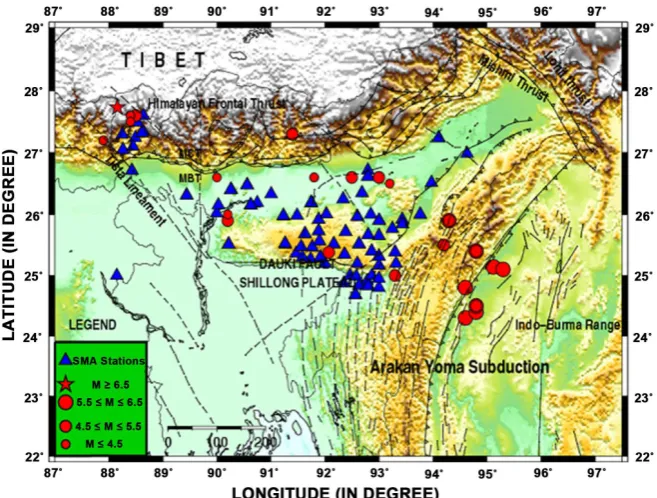
DOI: 10.4236/ojer.2018.72009 143 Open Journal of Earthquake Research Figure 1. Seismicity along with tectonics of the North-East Region, India.
Barapani Shear region, and Mikir Hills, Dhubri, Sylhet and Duaki faults, and
Dudhnai and Kulsi faults. The alignment of Kopili fault in NW-SE direction and
in North Dhansiri fault separates Mikir Hills from Shillong highlands
[21]
. The
NE India region is one of the seismically active regions of the world.
A strong motion accelerographs network has been installed in the region by
Department of Earthquake Engineering, Indian Institute of Technology,
Roor-kee with the objectives of studying the strong ground motions characteristics for
earthquake engineering purposes. The 598 accelerograms of 32 earthquakes (mb
3.9 - 6.8) recorded at this network has been used in the present analysis.
Figure
2
shows the locations of earthquakes and recording stations used in this study.
The lists of the earthquakes along with recording stations and geology are given
in
Table 1
.
3. Methodology
DOI: 10.4236/ojer.2018.72009 144 Open Journal of Earthquake Research Figure 2. Location of earthquakes and recording stations used in present study.
0
ln
A
=
ln
A
−
π
к
f
(2)
This a linear equation between “ln
A
” and frequency “
f
”. The “
κ
” can be
esti-mated from the slope (m) of the line (Equation (2)) as:
к
= −
m k
(3)
The following procedure has been adopted for the estimation of “
κ
”:
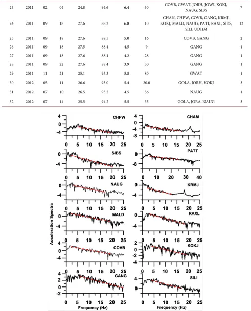
1) First the S-wave portion of the accelerogram is selected.
2) Fourier transform of the selected wave has been obtained using FFT and
plotted the same on log-linear scale
i.e.
with a logarithmic y-axis (amplitude)
and a linear x-axis (frequency).
3) Two frequencies have been selected by visual inspection of the spectrum of
S-waves: first at the start of linear downward trend in the spectrum (f1) and
second at the end of linear downward trend (f2). The visual inspection of S-wave
spectrum in selecting the two frequencies is preferred over the automatic
proce-dure as f1 and f2 vary from record to record. The visual inspection avoids the
biased estimates of “
κ
”. This procedure has been used in previous studies also
(e.g.
[28]
).
4) A line has fitted between f1 and f2 in a least square sense on log-linear plot.
The slope (m) of the line gives the value of “
κ
” (Equation (3)).
4. Results and Discussion
The values of “
κ
” have been estimated for the three components (N-S, E-W and
Z) of the recorded accelerograms using the procedure described above.
Figure 3
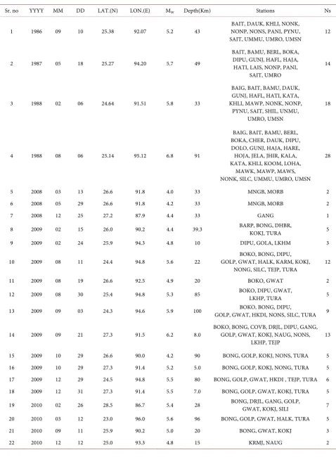
DOI: 10.4236/ojer.2018.72009 145 Open Journal of Earthquake Research Table 1. List of Earthquakes along with recording stations used to compute
κ
and Ns is number of stations.Sr. no YYYY MM DD LAT.(N) LON.(E) MW Depth(Km) Stations Ns
1 1986 09 10 25.38 92.07 5.2 43 NONP, NONS, PANI, PYNU, BAIT, DAUK, KHLI, NONK,
SAIT, UMMU, UMRO, UMSN 12
2 1987 05 18 25.27 94.20 5.7 49
BAIT, BAMU, BERL, BOKA, DIPU, GUNJ, HAFL, HAJA, HATI, LAIS, NONP, PANI,
SAIT, UMRO
14
3 1988 02 06 24.64 91.51 5.8 33
BAIG, BAIT, BAMU, DAUK, GUNJ, HAFL, HATI, KATA, KHLI, MAWP, NONK, NONP,
PYNU, SAIT, SHIL, UNMU, UMRO, UMSN
18
4 1988 08 06 25.14 95.12 6.8 91
BAIG, BAIT, BAMU, BERL, BOKA, CHER, DAUK, DIPU, DOLO, GUNJ, HAJA, HARE, HOJA, JELA, JHIR, KALA, KATA, KHLI, KOOM, LOHA,
MAWK, MAWP, MAWS, NONK, SILC, UMMU, UMRO, UMSN
28
5 2008 03 13 26.6 91.8 4.0 33 MNGB, MORB 2
6 2008 05 29 26.6 91.8 4.2 33 MNGB, MORB 2
7 2008 12 25 27.2 87.9 4.4 33 GANG 1
8 2009 02 15 26.0 90.2 4.4 39.3 BARP, BONG, DHBR, KOKJ, TURA 5
9 2009 02 24 25.9 94.3 4.8 10 DIPU, GOLA, LKHM 3
10 2009 08 11 24.4 94.8 5.6 22 GOLP, GWAT, HALK, KARM, KOKJ, BOKO, BONG, DIPU, NONG, SILC, TEJP, TURA 12
11 2009 08 19 26.6 92.5 4.9 20 BOKO, GWAT 2
12 2009 08 30 25.4 94.8 5.3 85 BOKO, DIPU, GWAT, LKHP, TURA 5
13 2009 09 03 24.3 94.6 5.9 100 GOLP, GWAT, HKDI, NONS, SILC, TURA BOKO, BONG, DIPU, 9
14 2009 09 21 27.3 91.5 6.2 8.0 BOKO, BONG, COVB, DRJL, DIPU, GANG, GOLP, GWAT, KOKJ, NAUG, NONS,
LKHP, TEJP 13
15 2009 10 29 26.6 90.0 4.2 90 BONG, GOLP, KOKJ, NONS, TURA 5
16 2009 10 29 27.3 91.4 5.2 5.0 BONG, GOLP, KOKJ, NONG, TURA 5
17 2009 12 29 24.5 94.8 5.5 80 BONG, GOLP, GWAT, HKDI , TEJP, TURA 6
18 2009 12 31 27.3 91.4 5.5 7.0 BONG, GOLP, GWAT, KOKJ, TURA 5
19 2010 02 26 28.5 86.7 5.4 28 BONG, DRJL, GANG, GOLP, GWAT, KOKJ, SILI 7
20 2010 03 12 23.0 96.0 5.6 96 BONG, GOLP, GWAT, HALK, TURA 5
21 2010 09 11 25.9 90.2 5.0 20 BONG, GWAT, KOKJ 3
DOI: 10.4236/ojer.2018.72009 146 Open Journal of Earthquake Research Continued
23 2011 02 04 24.8 94.6 6.4 30 COVB, GWAT, JORH, JOWI, KOKJ, NAUG, SIBS 7
24 2011 09 18 27.6 88.2 6.8 10 KOKJ, MALD, NAUG, PATI, RAXL, SIBS, CHAN, CHPW, COVB, GANG, KRMJ,
SILI, UDHM 13
25 2011 09 18 27.6 88.5 5.0 16 COVB, GANG 2
26 2011 09 18 27.5 88.4 4.5 9 GANG 1
27 2011 09 18 27.6 88.4 4.2 28 GANG 1
28 2011 09 22 27.6 88.4 3.9 30 GANG 1
29 2011 11 21 25.1 95.3 5.8 80 GWAT 1
30 2012 05 11 26.6 93.0 5.4 20.0 GOLA, JORH, KOKJ 3
31 2012 07 10 26.5 93.2 4.5 56 NAUG 1
32 2012 07 14 25.5 94.2 5.5 35 GOLA, JORA, NAUG 3
[image:6.595.53.545.84.694.2]DOI: 10.4236/ojer.2018.72009 147 Open Journal of Earthquake Research
It has been found that f1 lies in the range 2-13 Hz while f2 is in the range 20 - 28
Hz. The estimated values of “
κ
” corresponding to three components for the
earthquakes and recording stations are given in
Table 2
along with the site
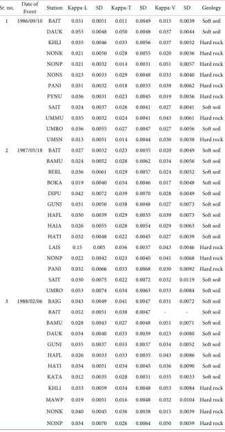
ge-ology. The standard deviations are also given in the table. The average values of
“
κ
” has been found to be 0.049 (L-component), 0.047 (T-component) and 0.040
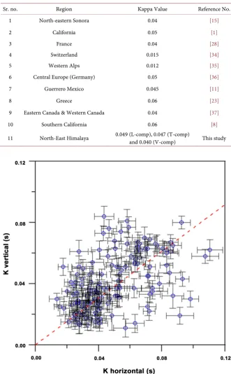
(V-component). A comparison between the
κ
values obtained from horizontal
and vertical components is shown in
Figure 4
. The values are found to be
simi-lar for most of the events. The vertical estimates are smaller than those of
hori-zontal estimates. This has been observed in other studies
[28]
[30]
. The values
obtained in the present study have been compared with those of other regions of
the world in
Table 3
. The estimates are found to be consistent.
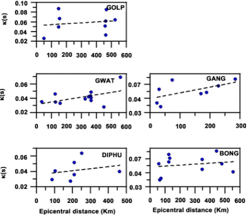
The distance dependence of
κ
has been analyzed using the following linear
model
[1]
:
0 R
к к
=
+
к
(4)
where
κ
0 is the value ofκ
at distance
R
= 0. This model has been used in many
studies due to its simplicity of formulation (e.g.
[1]
;
[28]
;
[31]
).
κ
0 is believed tobe station-dependent and may be related to the near surface attenuation. The
distance dependence of
κ
estimated from horizontal and vertical components is
shown in
Figure 5(a)
and
Figure 5 (b)
. The fitted linear model gives the
regres-sion.
0.037 0.0000158
к= + R
For vertical component
and
0.041 0.0000326
к= + R
For horizontal component
We note that distance dependence for both the components is not significant.
The values of
κ
0 as 0.041 (horizontal component) and 0.037 (verticalcompo-nent) represent the overall value for the region. The difference in these two
val-ues indicates that site response is different for different components as has been
observed in site amplification studies. The estimate of
κ
0 (vertical) is useful alongwith H/V ratio for the first order estimation of site effect where site-specific
bo-rehole data is not available as suggested by
[30]
.
Figure 6(a)
and
Figure 6(b)
show the distance dependence of
κ
on hard rock
sites and soft soil sites separately. The linear fit gives the following relations:
0.034 0.0000158
к= + R
For hard rock sites
and
0.037 0.000024
к= + R
For soft rock sites
DOI: 10.4236/ojer.2018.72009 148 Open Journal of Earthquake Research Table 2. The estimated values of
κ
for the three components of earthquakes along with recording stations with site geology.Sr. no. Date of Event Station Kappa-L SD Kappa-T SD Kappa-V SD Geology
1 1986/09/10 BAIT 0.031 0.0051 0.011 0.0049 0.015 0.0039 Soft soil DAUK 0.053 0.0048 0.050 0.0048 0.037 0.0044 Soft soil KHLI 0.035 0.0046 0.033 0.0056 0.037 0.0052 Hard rock NONK 0.021 0.0050 0.028 0.0055 0.020 0.0036 Hard rock NONP 0.021 0.0032 0.014 0.0031 0.051 0.0057 Hard rock NONS 0.023 0.0033 0.029 0.0048 0.033 0.0040 Hard rock PANI 0.031 0.0032 0.018 0.0033 0.039 0.0062 Hard rock PYNU 0.036 0.0031 0.023 0.0045 0.019 0.0056 Hard rock SAIT 0.024 0.0037 0.026 0.0041 0.027 0.0041 Soft soil UMMU 0.035 0.0032 0.024 0.0041 0.043 0.0061 Hard rock
UMRO 0.036 0.0055 0.027 0.0047 0.027 0.0056 Soft soil UMSN 0.013 0.0051 0.014 0.0044 0.030 0.0038 Hard rock 2 1987/05/18 BAIT 0.027 0.0032 0.023 0.0035 0.020 0.0049 Soft soil
DOI: 10.4236/ojer.2018.72009 149 Open Journal of Earthquake Research Continued
PYNU 0.041 0.0047 0.040 0.0059 0.014 0.0052 Hard rock SAIT 0.027 0.0038 0.023 0.0055 0.015 0.0049 Soft soil SHIL 0.033 0.0050 0.029 0.0046 0.024 0.0053 Hard rock UMMU 0.045 0.0109 0.060 0.0134 0.049 0.0124 Hard rock UMRO 0.037 0.0048 0.033 0.0035 0.041 0.0050 Soft soil UMSN 0.017 0.0040 0.019 0.0033 0.024 0.0043 Hard rock 4 1988/08/06 BAIG 0.056 0.0053 0.018 0.0051 - - Soft soil
BAIT 0.019 0.0040 0.019 0.0035 0.012 0.0126 Soft soil BAMU 0.026 0.0042 0.022 0.0036 0.033 0.0045 Soft soil BERL 0.034 0.0040 0.021 0.0032 0.021 0.0035 Soft soil BOKA 0.017 0.0039 0.007 0.0039 0.005 0.0035 Soft soil CHER 0.034 0.0037 0.032 0.0040 0.013 0.0034 Hard rock DAUK 0.036 0.0030 0.040 0.0034 0.021 0.0041 Soft soil
DIPU 0.026 0.0039 0.029 0.0036 0.047 0.0116 Soft soil DOLO 0.036 0.0037 0.042 0.0036 0.016 0.0043 Soft soil GUNJ 0.027 0.0033 0.026 0.0042 0.027 0.0049 Soft soil HAJA 0.046 0.0102 0.033 0.0083 0.027 0.0074 Soft soil HARE 0.031 0.0040 0.036 0.0037 0.027 0.0039 Soft soil HOJA 0.021 0.0037 0.034 0.0057 0.014 0.0067 Soft soil JELA 0.042 0.0047 0.045 0.0051 0.037 0.0043 Soft soil JHIR 0.038 0.0047 0.042 0.0056 0.034 0.0062 Soft soil KALA 0.036 0.0047 0.042 0.0056 0.034 0.0062 Soft soil KATA 0.074 0.0097 0.074 0.0098 0.035 0.0050 Soft soil KHLI 0.024 0.0073 0.022 0.0115 0.026 0.0045 Hard rock KOOM 0.036 0.0041 0.045 0.0061 0.040 0.0057 Soft soil
LOHA 0.041 0.0052 0.034 0.0057 0.029 0.0043 Soft soil MAWK 0.040 0.0082 0.029 0.0073 0.007 0.0105 Hard rock MAWP 0.026 0.0040 0.038 0.0037 0.018 0.0048 Hard rock MAWS 0.016 0.0031 0.015 0.0041 0.025 0.0062 Hard rock NONK 0.026 0.0032 0.030 0.0029 0.013 0.0056 Hard rock NONS 0.030 0.0081 0.042 0.0064 0.054 0.0071 Hard rock PANI 0.045 0.0087 0.020 0.0096 0.021 0.0048 Hard rock PYNU 0.035 0.0068 0.062 0.0082 0.019 0.0094 Hard rock SAIT 0.025 0.0048 0.022 0.0069 0.020 0.0108 Soft soil SHIL 0.028 0.0071 0.013 0.0082 0.046 0.0115 Hard rock SILC 0.039 0.0061 0.038 0.0054 0.035 0.0061 Soft soil UMMU 0.041 0.0084 0.044 0.0104 0.022 0.0143 Hard rock
UMRO 0.040 0.0061 0.039 0.0052 0.029 0.0043 Soft soil UMSN 0.026 0.0077 0.011 0.0076 0.022 0.0089 Hard rock 5 2008/03/13 MNG 0.044 0.0047 0.038 0.0038 0.024 0.0042 Soft soil
DOI: 10.4236/ojer.2018.72009 150 Open Journal of Earthquake Research Continued
6 2008/05/29 MNG 0.039 0.0034 0.036 0.0052 0.030 0.0048 Soft soil MOR 0.024 0.0041 0.028 0.0050 0.021 0.0053 Soft soil 7 2008/12/25 GANG 0.062 0.0068 0.081 0.0050 0.045 0.0073 Hard rock 8 2009/02/15 BARP 0.134 0.0195 0.116 0.157 0.020 0.0217 Soft soil
BONG 0.036 0.043 0.034 0.061 0.049 0.0071 Soft soil DHBR 0.051 0.0050 0.054 0.0049 0.051 0.0058 Soft soil KOKJ 0.055 0.0089 0.030 0.0054 0.025 0.0129 Soft soil TURA 0.063 0.0067 0.067 0.0055 0.067 0.0067 Soft soil 9 2009/02/24 DIPU 0.024 0.0056 0.035 0.0058 0.025 0.0042 Soft soil GOLA 0.051 0.0081 0.043 0.0075 0.030 0.0068 Soft soil LKHM 0.075 0.0081 0.076 0.0069 0.045 0.0095 Soft soil 10 2009/08/11 BOKO 0.046 0.0069 0.036 0.0069 0.017 0.0061 Soft soil BONG 0.061 0.0073 0.067 0.0057 0.061 0.0065 Soft soil DIPU 0.054 0.0066 0.049 0.0054 0.032 0.0064 Soft soil GOLP 0.070 0.0090 0.053 0.0082 0.057 0.0059 Soft soil GWAT 0.037 0.0052 0.044 0.0050 0.062 0.0059 Soft soil HALK 0.121 0.0097 0.136 0.0093 0.104 0.0116 Soft soil KARM 0.109 0.0073 0.112 0.0087 0.062 0.0068 Soft soil KOKJ 0.049 0.0052 0.042 0.0057 0.044 0.0074 Soft soil NONG 0.031 0.0051 0.017 0.0053 0.017 0.0053 Hard rock
SILC 0.105 0.0079 0.110 0.0094 0.058 0.0046 Soft soil TEJP 0.030 0.0065 0.029 0.0066 0.028 0.0076 Soft soil TURA 0.063 0.0069 0.063 0.0061 0.053 0.0056 Soft soil 11 2009/08/19 BOKO 0.029 0.0037 0.049 0.0039 0.025 0.0036 Soft soil GUAT 0.043 0.0031 0.041 0.0032 0.046 0.0035 Soft soil 12 2009/08/30 BOKA 0.029 0.0033 0.031 0.0034 0.020 0.0041 Soft soil DIPU 0.039 0.0037 0.041 0.0032 0.027 0.0026 Soft soil GUA 0.049 0.0036 0.048 0.0038 0.052 0.0040 Soft soil LKH 0.047 0.0037 0.054 0.0038 0.032 0.0036 Soft soil TURA 0.055 0.0031 0.059 0.0034 0.051 0.0036 Soft soil 13 2009/09/03 BOKA 0.026 0.0030 0.020 0.0037 0.007 0.0042 Soft soil BONG 0.052 0.0037 0.048 0.0047 0.068 0.0045 Soft soil DIPU 0.038 0.0042 0.034 0.0045 0.033 0.0037 Soft soil GOLP 0.027 0.0032 0.039 0.0035 0.032 0.0044 Soft soil GUA 0.042 0.0042 0.032 0.0040 0.036 0.0040 Soft soil HKD 0.090 0.0042 0.105 0.0041 0.061 0.041 Soft soil NONS 0.030 0.0046 0.023 0.0044 0.046 0.0045 Hard rock
DOI: 10.4236/ojer.2018.72009 151 Open Journal of Earthquake Research Continued
COBV 0.086 0.0037 0.075 0.0036 0.063 0.0050 Soft soil DJL 0.071 0.0040 0.095 0.0050 0.062 0.0045 Hard rock DIPU 0.055 0.0041 0.072 0.0039 0.056 0.0039 Soft soil GANG 0.067 0.0032 0.078 0.0039 0.051 0.0039 Hard rock GOLP 0.068 0.0033 0.065 0.0045 0.062 0.0040 Soft soil GUAT 0.051 0.0050 0.041 0.0051 0.058 0.0043 Soft soil KOKJ 0.048 0.0036 0.053 0.0046 0.063 0.0047 Soft soil NAUG 0.070 0.0028 0.075 0.0030 0.069 0.0036 Soft soil NONS 0.057 0.0044 0.051 0.0049 0.074 0.0062 Hard rock
DOI: 10.4236/ojer.2018.72009 152 Open Journal of Earthquake Research Continued
GWAT 0.028 0.0047 0.027 0.0071 0.061 0.0074 Soft soil HALK 0.095 0.0052 0.101 0.0056 0.030 0.0052 Soft soil TURA 0.062 0.0054 0.064 0.0055 0.054 0.0060 Soft soil 21 2010/09/11 BONG 0.032 0.0065 0.042 0.0048 0.049 0.0050 Soft soil GWAT 0.033 0.0044 0.033 0.0055 0.051 0.0046 Soft soil KOKJ 0.042 0.0059 0.044 0.0049 0.073 0.0048 Soft soil 22 2010/12/12 KRMJ 0.132 0.0077 0.144 0.0099 0.091 0.0078 Soft soil NAUG 0.060 0.0061 0.057 0.0058 0.049 0.0063 Soft soil 23 2011/02/04 COVB 0.059 0.0091 0.047 0.0082 0.038 0.0066 Soft soil GWAT 0.044 0.0040 0.034 0.0069 0.049 0.0047 Soft soil JORH 0.045 0.0039 0.035 0.0046 0.016 0.0050 Soft soil JOWI 0.049 0.0076 0.065 0.0073 0.011 0.0058 Soft soil KOKJ 0.030 0.0049 - - 0.033 0.0057 Soft soil NAUG 0.029 0.0047 0.034 0.0047 0.028 0.0052 Soft soil 24 2011/09/18 CHAM 0.064 0.0057 0.093 0.0067 0.040 0.0048 Hard rock
CHPW 0.081 0.0081 0.102 0.0093 0.019 0.0056 Hard rock COVB 0.069 0.0045 0.056 0.0043 0.037 0.0063 Soft soil GANG 0.057 0.0056 0.050 0.0061 0.046 0.0053 Hard rock
KRMJ 0.078 0.0055 0.084 0.0077 0.102 0.0084 Soft soil KOKJ 0.055 0.0063 0.054 0.0062 0.049 0.0080 Soft soil MALD 0.058 0.0044 0.060 0.0044 0.077 0.0068 Soft soil NAUG 0.062 0.0061 0.067 0.0044 0.053 0.0052 Soft soil PATI 0.057 0.0086 0.081 0.0068 0.070 0.0071 Hard rock RAXL 0.083 0.0039 0.061 0.0037 0.022 0.0061 Soft soil
SIBS 0.097 0.0077 0.098 0.0077 - - Soft soil SILI 0.079 0.0064 0.095 0.0074 0.032 0.0080 Soft soil UDHM 0.093 0.0067 0.077 0.0072 0.047 0.0064 Soft soil 25 2011/09/18 COVB 0.069 0.0066 0.097 0.0091 0.060 0.0075 Soft soil GANG 0.072 0.0058 0.032 0.0082 0.032 0.0076 Hard rock 26 2011/09/18 GANG 0.062 0.0054 0.054 0.0048 0.062 0.0101 Hard rock 27 2011/09/18 GANG 0.036 0.0053 0.041 0.0047 0.019 0.0071 Hard rock 28 2011/09/22 GANG 0.039 0.0051 0.028 0.0055 0.028 0.0062 Hard rock 29 2011/11/21 GWAT 0.035 0.0098 0.035 0.0098 0.017 0.0078 Soft soil 30 2012/05/11 GOLA 0.072 0.0186 0.026 0.0124 0.049 0.0153 Soft soil JORH 0.039 0.0085 0.040 0.0065 0.023 0.0070 Soft soil KOKJ 0.049 0.0057 0.043 0.0054 0.027 0.0058 Hard rock 31 2012/07/10 NAUG 0.045 0.0062 0.041 0.0085 0.057 0.0084 Soft soil 32 2012/07/14 GOLA 0.042 0.0051 0.033 0.0049 0.030 0.0063 Soft soil
DOI: 10.4236/ojer.2018.72009 153 Open Journal of Earthquake Research Table 3. Comparison of kappa value estimated in present study with those of different regions of world.
Sr. no. Region Kappa Value Reference No.
1 North-eastern Sonora 0.04 [15]
2 California 0.05 [1]
3 France 0.04 [28]
4 Switzerland 0.015 [34]
5 Western Alps 0.012 [35]
6 Central Europe (Germany) 0.05 [36]
7 Guerrero Mexico 0.045 [11]
8 Greece 0.06 [23]
9 Eastern Canada & Western Canada 0.04 [37]
10 Southern California 0.06 [8]
11 North-East Himalaya 0.049 (L-comp), 0.047 (T-comp) and 0.040 (V-comp) This study
Figure 4. A comparison between the
κ
values obtained from horizontal and vertical components.DOI: 10.4236/ojer.2018.72009 154 Open Journal of Earthquake Research (a) (b)
Figure 5. (a) Dependency of kappa (Horizontal) on Epicentral Distance; (b) Dependency of kappa (Vertical) on Epicentral Dis-tance.
(a) (b) Figure 6. (a) Distance dependence of
κ
for hard rock sites; (b) Distance dependence ofκ
for soft soil sites.0.034 0.0000158
к= + R for hard rock sites and к 0.037 0.000024= + R for soft soil sites.
[image:14.595.59.540.67.235.2] [image:14.595.60.540.281.423.2] [image:14.595.180.428.477.692.2]DOI: 10.4236/ojer.2018.72009 155 Open Journal of Earthquake Research (a)
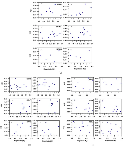
[image:15.595.63.542.66.632.2](b) (c) Figure 8. Magnitude dependency of kappa at some of the stations.
DOI: 10.4236/ojer.2018.72009 156 Open Journal of Earthquake Research
formations as suggested by
[33]
.
The dependence of kappa values on earthquake size has been examined by
plotting the estimated
κ
values with earthquake magnitudes for the stations
where sufficient number of earthquake have been recorded.
Figure 8(a)-(c)
show such plots for some of the stations. We note that there is a scatter and the
correlation between “
κ
” and magnitude at most of the stations for the region
under study is not significant. This suggests that that “
κ
” is not related to source
effect for NE Himalaya region.
[31]
has reported similar property of
κ
for
small-er magnitude earthquakes occurred in Kachchh region of Gujarat, India. The
analysis in the present study indicates that kappa for NE region is related with
the high frequency attenuation in the top surface layer. One of the scientific
dis-cussions about
κ
is whether it is due to source effect or site effect or both. The
different studies show different results for different regions of the world. The
present study based on the available data found that
κ
is related to site effect in
NE region. This is empirical inference drawn on the basis of recorded waveforms
in the region. The same may be validated with more data whenever available.
5. Conclusions
The average value of
κ
estimated from the spectral analysis of horizontal
com-ponents of 598 accelerograms for NE India region has been found to be in the
range 0.047 - 0.049 and 0.040 for vertical component. The distance dependence
of
κ
is not significant. The
κ
0(soft site)/κ
0(rock site) ratio is found to be 1.09. Theanalysis shows that
κ
is not dependent on the magnitude but dependent on
site-condition in the region for the range of magnitudes studies here. The study
presents the
κ
model for NE India region which is first study of its kind in the
region. The inferences drawn about
κ
in the NE region are based on the data
available for the analysis. The same may be validated further as and when more
data is available. With more data, the spatial distribution may also be
investi-gated in the region. The other methods reported in the literature may also be
applied to estimate
κ
in the region.
The estimated values of
κ
are useful in the studies of Ground Motion
Predic-tion EquaPredic-tions (GMPE) as well as for the simulaPredic-tion of earthquake strong
ground motions in the seismically active NE region. Thus this study is important
for bearing on the seismic hazard studies of the region.
Acknowledgements
The authors are thankful to their respective organizations for support. The
au-thors are very grateful to Dr. RBS Yadav for his kind help in this research. The
waveform of events has been downloaded from the site
http://www.pesmos.in
.
The authors are thankful to the reviewers and the editor for their extremely
con-structive comments which helped in improving the manuscript significantly.
References
Am-DOI: 10.4236/ojer.2018.72009 157 Open Journal of Earthquake Research plitude Spectrum of Acceleration at High Frequencies. Bulletin of the Seismological
Society of America, 74, 1969-1993.
[2] Brune, J.N. (1970) Tectonic Stress and Spectra of Seismic Shear Waves for Earth-quakes. Journal of Geophysical Research, 75, 4997-5009.
https://doi.org/10.1029/JB075i026p04997
[3] Hanks, T.C. and McGuire, R.K. (1981) The Character of High Frequency Strong Ground Motion. BSSA, 71, 2071-2095.
[4] Hanks, T.C.M. (1982)
f
max.
Bulletin of the Seismological Society of America, 72,
1867-1879.[5] Papageorgiou, A.S. and Aki, K. (1983) A Specific Barrier Model for the Quantative Description of Inhomogeneous Faulting and Prediction of Strong Motion. I. De-scription of Model. Bulletin of the Seismological Society of America, 73, 693-722. [6] Singh, S.K., Apsel, R.J., Fried, J. and Brune, J.N. (1982) Spectral Attenuation of SH
Waves along the Imperial Fault. Bulletin of the Seismological Society of America, 72, 2003-2016.
[7] Anderson, J.G. (1986) Implication of Attenuation for Studies of the Earthquake Source. In: Das, S., Boatwright, J. and Scholz, C.H., Eds.,
Earthquake Source
Me-chanics, Maurice Ewing Series 6, American Geophysical Union, Washington DC,
311-318. https://doi.org/10.1029/GM037p0311[8] Anderson, J.G. (1991) A Preliminary Descriptive Model for the Distance Depen-dence of the Spectral Decay Parameter in Southern California. Bulletin of the
Seis-mological Society of America, 81, 2186-2193.
[9] Tsai, C.-C.P. and Chen, K.-C. (2000) A Model for the High-Cut Process of Strong Motion Acceleration in Terms of Distance, Magnitude and Site Condition: An Ex-amples from the SMART1 Array, Lotung, Taiwan. Bulletin of the Seismological
So-ciety of America, 90, 1535-1542.
https://doi.org/10.1785/0120000010[10] Petukhin, A. and Irikura (2000) A Method for the Separation of Source and Site Ef-fects and the Apparent Q Structure from Strong Ground-Motion Data. Geophysical
Research Letters, 27, 3429-3432.
https://doi.org/10.1029/2000GL011561[11] Purvance, M.D. and Anderson, J.G. (2003) A Comprehensive Study of the Observed Spectral Decay in Strong-Motion Accelerations Recorded in Guerrero, Mexico.
Bulletin of the Seismological Society of America, 93, 600-611.
https://doi.org/10.1785/0120020065
[12] Halldorsson, B. and Papageorgiou, A.S. (2005) Calibration of the Specific Barrier Model to Earthquakes of Different Tectonic Regions. BSSA, 95, 1276-1300.
https://doi.org/10.1785/0120040157
[13] Boore, D.M. (2003) Simulation of Ground Motion Using the Stochastic Method.
Pure and Applied Geophysics, 160, 635-676.
https://doi.org/10.1007/PL00012553[14] Cotton, F., Scherbaum, F., Bommer, J.J. and Bungum, H. (2006) Criteria for Select-ing and AdjustSelect-ing Ground-Motion Models for Specific Target Regions: Application to Central Europe and Rock Sites. Journal of Seismologys, 10, 137-156.
https://doi.org/10.1007/s10950-005-9006-7
[15] Fernandez, A.I., Castro, R. and Huerta, C.I. (2010) The Spectral Decay Parameter Kappa in Northeastern Sonora, Mexico.
Bulletin of the Seismological Society of
America, 100, 196-206.
https://doi.org/10.1785/0120090049DOI: 10.4236/ojer.2018.72009 158 Open Journal of Earthquake Research
https://doi.org/10.1785/0120120093
[17] Campbell, K.W. (2003) Prediction of Strong Ground Motion Using the Hybrid Em-pirical Method and Its Use in the Development of Ground Motion (Attenuation) Relations in Eastern North America. Bulletin of the Seismological Society of
Amer-ica, 93, 1012-1033.
https://doi.org/10.1785/0120020002[18] Atkinson, G.M. and Boore, D.M. (2006) Earthquake Ground Motions Prediction Equations for Eastern North America.
Bulletin of the Seismological Society of
America, 96, 2181-2205.
https://doi.org/10.1785/0120050245[19] Dasgupta, S., Pande, P., Ganguly, D., Iqbal, Z., Sanyal, K., Venaktraman, N.V., Dasgupta, S., Roy, A., Das, L.K., Misra, P.S. and Dupta, H. (2000) Seismotectonic Atlas of India and Its Environs. Geological Survey of India, Calcutta, India.
[20] Nandy, D.R. (2001) Geodynamics of North Eastern India and the Adjoining Region. ACB Publications, Kolkata.
[21] Thingbaijam, K.K.S., Nath, S.K., Yadav, A., Raj, A., Walling, M.Y. and Mohanty, W.K. (2008) Recent Seismicity in North-East India and Its Adjoining Region.
Jour-nal of Seismology, 12, 107-123.
https://doi.org/10.1007/s10950-007-9074-y[22] Biasi, G.P. and Smith, K.D. (2001) Site Effects for Seismic Monitoring Stations in the Vicinity of Yucca Mountain, Nevada. MOL20011204.0045, A Report Prepared for the US DOE/University and Community College System of Nevada (UCCSN) Cooperative Agreement.
[23] Margaris, B.N. and Boore, D.M. (1998) Determination of
σ and κ
0 from Response Spectra of Large Earthquake in Greece.Bulletin of the Seismological Society of
America, 88, 170-182.
[24] Drouet, S., Cotton, F. and Guéguen, P. (2010) VS30,
κ, Regional Attenuation and
Mw from Accelerograms: Application to Magnitude 3-5 French Earthquakes.Geo-physical Journal International, 182, 880-898.
https://doi.org/10.1111/j.1365-246X.2010.04626.x
[25] Oth, A., Bindi, D., Parolai, S. and Di Giacomo, D. (2011) Spectral Analysis of K-NET and KiK-Net Data in Japan, Part II: On Attenuation Characteristics, Source Spectra, and Site Response of Borehole and Surface Stations.
Bulletin of the
Seis-mological Society of America, 101, 667-687.
https://doi.org/10.1785/0120100135[26] Anderson, J.G. and Humphrey Jr., J.R. (1991) A Least-Squares Method for Objec-tive Determination of Earthquake Source Parameters.
Seismological Research
Let-ters, 62, 201-209.
https://doi.org/10.1785/gssrl.62.3-4.201[27] Humphrey Jr., J.R. and Anderson, J.G. (1992) Shear Wave Attenuation and Site Re-sponse in Guerrero, Mexico. BSSA, 81, 1622-1645.
[28] Douglas, J., Gehl, P., Bonilla, L.F. and Gelis, C., (2010) A
κ
Model for Mainland France. Pure and Applied Geophysics, 167, 1303-1315.https://doi.org/10.1007/s00024-010-0146-5
[29] Van Houtte, C., Drouet, S. and Cotton, F. (2011) Analysis of the Origins of κ (kap-pa) to Compute Hard Rock to Rock Adjustment Factors for GMPEs. Bulletin of the
Seismological Society of America, 101, 2926-2941.
https://doi.org/10.1785/0120100345
[30] Motazedian, D. (2006) Region-Specific Key Seismic Parameters for Earthquakes in Northern Iran. Bulletin of the Seismological Society of America, 96, 1383-1395.
https://doi.org/10.1785/0120050162
DOI: 10.4236/ojer.2018.72009 159 Open Journal of Earthquake Research 442-455. https://doi.org/10.1080/19475705.2018.1447025
[32] Kilb, D., Biasi, G., Anderson, J., Brnue, J., Peng, Z. and Vernon, F.L. (2012) Spectral Decay Parameter Kappa for Small and Moderate Earthquakes Using Southern Cali-fornia ANZA Seismic Network Data. Bulletin of the Seismological Society of
Amer-ica, 102, 284-300.
https://doi.org/10.1785/0120100309[33] Lai, W., Wei, X., Feng, N.N., Shuping, C., Feng, L. and Qiumei, G. (2016) Research on Seismic Performance of Reinforced Concrete Frame with Unequal Span under Low Cyclic Reversed Loading. The Open Civil Engineering Journal, 10, 373-383.
https://doi.org/10.2174/1874149501610010373
[34] Bay, F., Fah, D., Malagnini, L. and Giardini, D. (2003) Spectral Shear-Wave Ground Motion Scaling in Switzerland. Bulletin of the Seismological Society of America, 93, 414-429. https://doi.org/10.1785/0120010232
[35] Morasca, P., Malagnini, L., Akincl, A., Spallaroosa, D. and Hermann, R.B. (2006) Ground Motion Scaling in Western Alps. Journal of Seismology, 10, 315-333.
https://doi.org/10.1007/s10950-006-9019-x
[36] Malagnini, L., Herrmann, R.B. and Koch, K. (2000) Regional Ground Motion Scal-ing in Central Europe.