Comparative Evaluation of Spatial Interpolation Methods for Estimation of Missing Meteorological Variables over Ethiopia

http://www.scirp.org/journal/jwarp ISSN Online: 1945-3108

ISSN Print: 1945-3094

Comparative Evaluation of Spatial

Interpolation Methods for Estimation of

Missing Meteorological Variables over Ethiopia

Andualem Shigute Boke

Department of Hydraulic and Water Resources Engineering, Jimma Institute of Technology, Jimma University, Jimma, Ethiopia

Abstract

In developing countries like Ethiopia where there is abundant water resources potential and also luck of reliable meteorological quality data, it expected to face the problem of missing meteorological data. Therefore, in conducting any water resources studies in any river basin for water resource project planning and management (like small scale irrigation), the first step before starting data analysis is to fill up the missing values of the meteorological variables (like rainfall, temperature, sunshine, wind speed etc.) which are required to start the study. One way of filling these missing variables is using datasets from other stations in the surrounding and applying appropriate spatial interpola-tion methods. A lot of studies have been conducted around the world to iden-tify which method is the best to be applied to particular study area among the available spatial interpolation techniques. But when we come to Ethiopia, the study area, few or no studies are conducted to recommend the best performed method. Therefore, the objective of this paper is to conduct comparative evaluation of five interpolation techniques Nearest Neighbour (NN), Inverse Distance Weighting Average (IDWA), Modified Inverse Distance Weighting Average (MIDWA), Kriging Method (KM) and Thin Plate Spline (TPS) for estimation of four climatic variables (rainfall, mean temperature, wind speed and sunshine fraction) over complex topography of Ethiopia. Performance assessment is done using Mean Error (ME), Mean Absolute Error (MAE), Mean Relative Error (MRE) and Root Mean Square Error (RMSE); and the number of the meteorological stations selected for validation is ten (10) and these are distributed over the study area taking into account the variation of elevation ranging from 860 m (Awash) to 2420 m (Debremarkos) above sea level. The radial distances of 100 km and 200 km were selected and it was found that 100 km radial distance was not appropriate to compare all methods as some variables could not be estimated by KM and TPS. Therefore, 200 km was selected for further analysis and the result showed that NN, IDWA, and How to cite this paper: Boke, A.S. (2017)

Comparative Evaluation of Spatial Interpo-lation Methods for Estimation of Missing Meteorological Variables over Ethiopia. Jour-nal of Water Resource and Protection, 9, 945-959.

https://doi.org/10.4236/jwarp.2017.98063

Received: January 20, 2017 Accepted: July 1, 2017 Published: July 4, 2017

Copyright © 2017 by author and Scientific Research Publishing Inc. This work is licensed under the Creative Commons Attribution International License (CC BY 4.0).

MIDWA were best methods relative to the remaining two methods (KM and TPS) for all variables and all stations except at Dire Dawa and Addis Ab-aba-Bole for estimation of wind speed using all methods except NN, and rain-fall using TPS, respectively. Hence, NN, IDWA, and MIDWA methods could be used for estimation of missing meteorological variables over Ethiopia whenever necessary.

Keywords

Spatial Interpolation, Meteorological Variables, Comparative Evaluation, Ethiopia

1. Introduction

In developing countries like Ethiopia where there is sufficient amount of water resources potential and also luck of high quality meteorological data, it expected to have the problem of facing missing meteorological data even though all means were used to avoid these missing values from the records [1] [2]. Some of the causes of the occurrence of these data problem could be absence of observer, malfunction of instruments, incorrect measurements, relocation of stations, and loss of records [3] [4].

During conducting any hydrological and environmental studies/modeling in any river basin for water resources project planning and management, the first step before starting data analysis is to fill up the missing values of the meteoro-logical variables (like rainfall, temperature, sunshine, wind speed etc.) required for the study [5]. Unless these missing values are filled up by appropriate me-thods so as to make the dataset complete, the data used may be biased and can lead to wrong conclusions [6]. One way of filling these missing meteorological variables at targeted station is using datasets from other selected stations in the surrounding and applying appropriate spatial interpolation methods [7]. There are more than 42 interpolation methods available in the literature [8]. In order to get good results of estimation, it is a must to select best interpolation tech-nique for the study selected as the interpolation techtech-niques are affected by dif-ferent factors like sample size of the data, the sampling design and data proper-ties [8].

At global scale [9] used Thin-Plate Spline method as interpolation technique to generate global (excluding Antarctica) monthly data for precipitation, and mean, minimum and maximum temperature using data collected from different sources in the period 1950-2000.

[11] conducted a comparative study on four interpolation methods (Ordinary Kriging, Inverse Distance Squared, Gradient-Plus-Inverse-Distance Squared and Residual Kriging) for predicting reference evapotranspiration over Greece terri-tory and found that Gradient-Plus-Inverse-Distance Squared performed best and the result from Residual Kriging is not optimal even though it performed better than Inverse Distance Squared and Ordinary Kriging. The evaluation sta-tistics used are the mean error, mean absolute error and root mean squared er-ror.

A study carried out by [12] over South Africa to evaluate performance of four spatial interpolation methods (Inverse Distance Weighting, Ordinary Kriging, Univariate Kriging and Co Kriging) using annual rainfall collected from 545 sta-tions and the result showed that Ordinary Kriging performed best compared to other three methods.

[13] developed multiple regression models for generating mean annual rain-fall as a function of elevation and geographic location for 63 Ethiopian meteoro-logical stations using datasets from 1969 up to 1985. In this study, regionaliza-tion is the main technique applied to generate mean annual rainfall.

[14] evaluated four spatial interpolation techniques (Arithmetic Mean, AM; Normal Ratio, NR; Inverse Distance Weighting, IDW and Coefficient of Corre-lation Weighting, CCW) for filling missing daily rainfall over upper Blue Nile river particularly on Gumera watershed using daily rainfall data (1987-2008) collected from nine stations and found that AM and CCW methods had shown better performance. On the lowland plain and near to Lake Tana it is AM while upstream and on the mountainous areas it is CCW that showed better perfor-mance where as NR is not good method to this area.

When we come to the selected study area, Ethiopia, very little studies are conducted on the selection of spatial interpolation techniques for estimating missing variables which could be used as input to some hydrological and other water related models. Before selecting among the available interpolation tech-niques, it is important to properly test their performance over the selected study so as to get best results relatively.

In areas where there is insufficient number of meteorological stations, it would be difficult to find continuously recorded meteorological datasets. In such cases there should be an alternative source of data to be used for water resources and environmental studies or modeling. One source of such data type is FAO database developed for the globe data collected by World Meteorological Service Agency; and New_LocClim_1.10 (Local Climate Estimator version 1.10) [15] is one of those databases. In this database there are nine spatial interpolation techniques available and nothing is known which one is best for which part of the world; hence the result obtained from one method will give different results as compared to the results that could be obtained from another method for the same station.

variables found in FAO database (New_LocClim_1.10); and then to recom-mend the best performing interpolation methods to be used in Ethiopia.

2. Materials and Methods

2.1. Description of Study Area

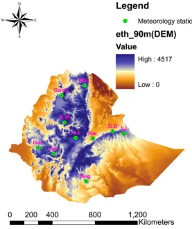
The selected study area is Ethiopia located in East Africa. The country has very complex variation of topography and geology. The elevation of the area varies from 126 meters below sea level (Dalol depression) and 4620 meters above sea level (Mount Ras Dashen). The surface area of the country is 1.13 million square kilometers and 99.3% (land) and 0.7% is covered by water bodies (Lakes). This country is well known for its water resources potential. It has 12 major river ba-sins and the amount of water resources available as surface run and ground wa-ter potential per year is estimated to be 122 BCM and 2.6 - 6.5 BCM, respectively [16]. The other important point is that there is very high spatial and temporal rainfall variation across the country which resulted in uneven distribution of the water resources of the country throughout the year. According to [17] the popu-lation of Ethiopia is 102,765,596 (19.8 % in urban and 80.2% in rural areas) by 2016. Study area map with selected base meteorological stations is given in Fig-ure 1.

2.2. Data

Datasets used in this study area are taken from FAO database called Local Cli-mate Estimator (or New_LocClim_1.10, as it is briefly explained in Introduc-tion part of this paper) prepared for the globe based on data collected from me-teorological stations around the world [15]. The datasets included in this tool are of two types (observed data in monthly scale; synthetic dataset in daily& monthly scale) eight (8) meteorological variables (rainfall, wind speed, mean temperature, maximum temperature, minimum temperature, vapor pressure, and sunshine fraction) both for observed and synthetic datasets; and both of the datasets are long-term average values. In the same tool, nine (9) interpolation methods were built in for generation of synthetic data.

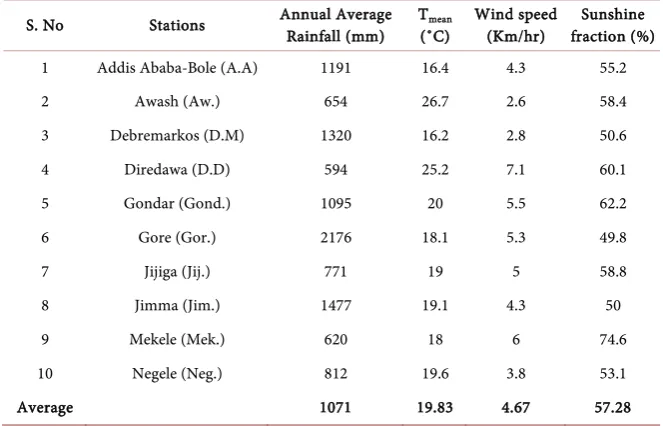
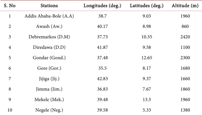
Among the eight (8) variables found in the tool, only four (rainfall, mean temperature, wind speed, and sunshine fraction) commonly used variables were included in the study. The long-term average monthly observed dataset is given in Table 1 for selected 10 reference meteorological stations for validation [18]; and the name and geographic locations of the selected meteorological stations are described in Table 2 and spatial distribution is shown in Figure 1.

During selection of the validation stations, an attempt has been made to in-clude elevation ranges from 860 m (Awash) up to 2420 m (Debremarkos) so as to see the influence of topography on the accuracy of interpolators and their re-presentativeness for the whole country. The same is true for the Longitude and Latitude. In Table 1, long year average values of observed meteorological data of the selected stations are shown.

2.3. Spatial Interpolation Methods

According to [8], all interpolation techniques available in literature (more than 42) are classified in one of the following categories: i) Geostatistical ii) Non-

Table 1. Observed long-term average values of meteorological variables at selected vali-dation stations.

S. No Stations Annual Average _{Rainfall (mm)} Tmean

(˚C) Wind speed (Km/hr) fraction (%) Sunshine

1 Addis Ababa-Bole (A.A) 1191 16.4 4.3 55.2

2 Awash (Aw.) 654 26.7 2.6 58.4

3 Debremarkos (D.M) 1320 16.2 2.8 50.6

4 Diredawa (D.D) 594 25.2 7.1 60.1

5 Gondar (Gond.) 1095 20 5.5 62.2

6 Gore (Gor.) 2176 18.1 5.3 49.8

7 Jijiga (Jij.) 771 19 5 58.8

8 Jimma (Jim.) 1477 19.1 4.3 50

9 Mekele (Mek.) 620 18 6 74.6

10 Negele (Neg.) 812 19.6 3.8 53.1

Table 2. Name and geographic location of selected base meteorological stations.

S. No Stations Longitudes (deg.) Latitudes (deg.) Altitude (m)

1 Addis Ababa-Bole (A.A) 38.7 9.03 1960

2 Awash (Aw.) 40.17 8.98 860

3 Debremarkos (D.M) 37.73 10.35 2420

4 Diredawa (D.D) 41.87 9.58 1100

5 Gondar (Gond.) 37.48 12.65 2300

6 Gore (Gor.) 35.5 8.17 1680

7 Jijiga (Jij.) 42.83 9.37 1660

8 Jimma (Jim.) 36.83 7.67 1860

9 Mekele (Mek.) 39.48 13.5 1960

10 Negele (Neg.) 39.58 5.33 1380

Geostatistical or iii) combined. Based on the number of variables involved, Geostatistical categories could be univariate or multivariate. In the univariate type, only the primary variables are considered for interpolation whereas in case of the multivariate other secondary variables (such as elevation) are included. The algorithm used in all spatial interpolation methods is similar.

Based on the work of [8], the general formulation used in all the available in-terpolation methods is similar and the formulation is as follows:

( )

( )

n

o o i i i

Z x =

∑

µ

where:

Zo = estimated value of an attribute or variable at point of interest xo,

z = observed value at the sampled point (xi); µ = weight assigned to the sampled point;

n = number of sampling points used for estimation;

xi = represents geographic coordinate (x, y) at location i.

Therefore, one interpolation is different from the other only by the methods used to estimate the weighting factor, µ. The theoretical background of each of the selected methods will be described one by one as in the coming subsections.

2.3.1. Nearest Neighbor (NN)

In this method of estimation sampling point nearest to the missing point are considering in such a way that perpendicular bisectors are drawn between sam-pling points so as to form polygons (like Thiessen polygon). Then each of the sampling points will have one polygon and the sampling point will be located at the center of the polygon. Points located in each of the polygons will have equal weight. If we designated these polygons by V V V1, 2, 3,,Vn then weighting

fac-tors (μ) described in Section 2.3 are formulated as follows [8]: 1 if

0 otherwise

i i

i

x V

µ

Therefore, for estimating missing meteorological variable at point of the in-terest this method will assign 1as a weight for sampling point located in the po-lygon and otherwise 0.

Then the general formulation remains the same as briefly explained in the Equation (1) above.

2.3.2. Inverse Distance Weighing Average (IDWA)

In this method estimation of missing value of meteorological variables at the point of interest is done by a linear combination of the weighted mean of meas-ured variables at surrounding stations as inverse function of the distance of point of the interest from surrounding meteorological stations. The binding as-sumption in this method is that the closer the surrounding station to point of interest the more similar the corresponding meteorological variables will be and vice verse [8].

1 1 1 p i i n p i i d d µ = =      _ 

∑

where:

di: distance between surrounding station and station where the variable is

missing;

n: is the number of surrounding stations where the corresponding variable has measured value;

p: is power (influential parameter on IDWA factor and commonly 2);

µi: weighting factor assigned to each of the stations based on their distance

from the point of Interest.

2.3.3. Modified Inverse Distance Weighing Average (MIDWA)

As the name implies Modified Inverse Distance Weighting Average (MIDWA) method is the modified form of IDWA method. The modification is done on the weighting factor by introducing the effect of elevation difference. If the elevation difference between the base station and the surrounding station is large, the ef-fect of elevation difference will have an efef-fect on estimated value of the meteo-rological variable. [19] replaced the weighting factor in the IDWA method by introducing the ratio of distance to elevation difference as follows and keeping the other factors similar to IDWA method. The same author mentioned that this relation is good to mountainous areas (like Ethiopia, study area). A little mod-ification of symbols has been made to be consistent with IDWA method.

1 p i i i p n _i i i d H d H µ =   _∆    =   _∆   

∑

missing;

n: is the number of surrounding stations where the corresponding variable has measured value;

p: is power (influential parameter on IDWA factor and commonly 2);

∆_{Hi: the elevation difference between the base station and the surrounding}

stations;

µi: weighting factor assigned to each of the stations based on the ratio (di/∆_Hi).

2.3.4. Kriging Method (KM)

The commonly used kriging method among the kriging families is ordinary kriging. In this estimation method, optimal and unbiased estimation of regiona-lized variables at unsampled location is carried out and the nature of the data at the sampled locations should be free of trend [11]. The general formulation de-veloped in Equation (1) is applicable here also.

( )

( )

n

o i i i

ž X =

∑

µ

where:

( )

ž X = estimated value of an attribute or variable at point of interest Xo,

z = observed value at the sampled point (xi); µ_{= weight assignedto the sampled point;}

n = number of sample points used for estimation;

xi = represents geographic coordinate (x, y) at location i.

The considerations taken in assigning weights in kriging are two: 1.The estimate, ž X

( )

( )

( )

E_ž X −Z X _=

2.The prediction variance is minimum:

( )

( )

( )

2

0 minimum

o o

X Varž X Z X 

∂ = _ − _=

2.3.5. Thin-Plate-Spline (TPS)

To estimate missing values of any meteorological variable at base station, Thin- Plate-Spline method is one option among the available methods. As it is ex-plained in [13], the basic equation for Partial Spline method for n number of measurement stations for the variable of interest to be estimated at base station,

say X0, represented by Zo is given as follows:-

( )

(

)

1, ,

o i i i

Z =F x +D Y +β i=  n (6)

where:

Zo: predicted value of a missing meteorological variable at base station;

xi: is a d-dimensional vector of independent variable;

F: is an unknown smooth function of the xi;

Yi: is a p-dimensional vector of independent co-variates;

D: is an unknown p-dimensional vector of coefficient of the Yi;

i

β _{: is zero mean randomerror term.}

Spline method) when the value of p is zero (or, p = 0), which means there is no covariance. Therefore, for this particular study Thin-Plate-Spline method is se-lected and this method is relatively robust and developed for climatic data [8].

Summary of the selected methods for this study with their corresponding ab-breviations is given below in Table 3.

2.4. Assumptions, Limitations and Suitability of Spatial

Interpolation Methods

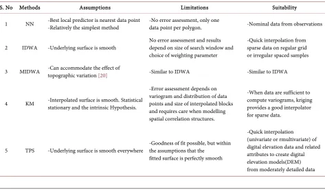
Each of the selected spatial interpolation methods has both merits and demerits; and Table 4 shows summary of these.

2.5. Evaluation of Spatial Interpolation Methods

In [8] [11], different methods of spatial interpolation techniques were well re-viewed but all of the studies could not reveal which method is the best method to be applied worldwide and for all discipline as the accuracy of the methods is af-fected by different factors rather than only on the interpolator itself. Therefore, it

Table 3. Spatial interpolation methods used for the study.

S. No. Name of methods Abbreviations used

1 Nearest neighbor NN

2 Inverse distance weighing average IDWA

3 Modified inverse distance weighing average MIDWA

4 Kriging method KM

5 Thin-Plate-Spline TPS

Table 4. Theoretical comparison of spatial interpolation methods: assumptions, limitations and suitability [8] [20].

S. No Methods Assumptions Limitations Suitability

1 NN -Best local predictor is nearest data point _{-Relatively the simplest method} -No error assessment, only one _{data point per polygon.} -Nominal data from observations

2 IDWA -Underlying surface is smooth No error assessment and results depend on size of search window and choice of weighting parameter

-Quick interpolation from sparse data on regular grid or irregular spaced samples

3 MIDWA -Can accommodate the effect of _{topographic variation [20]} -Similar to IDWA -Similar to IDWA

4 KM -Interpolated surface is smooth. Statistical _{stationary and the intrinsic Hypothesis.}

-Error assessment depends on variogram and distribution of data points and size of interpolated blocks and requires care when modelling spatial correlation structures.

-When data are sufficient to compute variograms, kriging provides a good interpolator for sparse data.

5 TPS -Underlying surface is smooth everywhere -Goodness of fit possible, but within the assumptions that the fitted surface is perfectly smooth

is important to select the appropriate interpolator for a specific study area before carrying out the interpolation process and one way of making this is an evalua-tion of each of the interpolaevalua-tion methods selected so as to identify which method is giving us the best estimates among the selected methods for our study. The commonly used way of evaluating performance of these interpolation techniques is using the concept of cross validation which can be expressed by commonly used statistical indicators [2] [11] [20] [21] [22] and they are described as fol-lows:

1.Mean Error (ME): shows the degree of bias between the measured and pre-dicted variable.

2.Mean Absolute Error (MAE): indicates the measure of how far is the pre-dicted value from error regardless of the sign.

3.Mean Relative Error (MRE): provides how far the predicted value is from error relative to the measured value.

4.Root Mean Square Error (RMSE): Shows how sensitive is the predicted value towards outliers. The formula for each of the above mentioned statistical in-dicators are given below:

(

)

(

( )

( )

)

1

Mean Error ME n _{o i i}

i Z X Z X

n =

=

∑

(

)

( )

( )

1

Mean Absolute Error MAE _in Z_o X_i Z X_i

n =

=

∑

(

)

(

( )

( )

)

1 1

Root Mean Square Error RMSE ni Zo Xi Z Xi

n =

=

∑

(

)

( )

_{( )}

( )

Mean Relative Error MRE n_i o i i

i

Z X Z X

n = Z X

−

=

∑

where:

n: is number of data points ( or stations) in consideration;

Zo: predicted value of a missing meteorological variable at base station;

Z: measured value of corresponding meteorological variable at base station;

Xi: is geographic coordinates (x, y) at station i.

3. Results and Discussion

3.1. Radius of Influence, r = 100 km

According to recommendation of [23], as the first attempt, the radius of influ-ence was specified as 100 km and some observation was made and the following results were obtained:

First, for common radial distance, r = 100 km ,the number of sampling sta-tions selected for all variables, for all stasta-tions, and for all interpolation methods is the same and it is 10.

Spline (TPS) nearly for all stations. With regard to variables, for the selected ra-dius of influence it was not possible to get estimation values for rainfall at De-bremarkos, Gondar, and Negele for KM and TPS. For all variables, it was im-possible to predict values using KM for Awash station. For wind speed, KM is not good method nearly for all stations.

Third, the three methods (NN, IDWA, and MIDWA) have nearly similar performance and very close to the observed values for all variables at all stations; therefore, these methods could be used for estimating missing meteorological variables over the country Ethiopia whenever it is important.

Fourth, the analysis done for each of the considered station is not complete due to very limited number of stations with in 100 km radius for estimating some variables at selected stations. Therefore, another option was proposed to carry out complete and confidential analysis; and this is to increase the radius of influence from 100 km to 200 km, as there are similar studies conducted in another part of the world using radial distance more than 100 km [24] [25] [26] and conduct the analysis again so as to see if there is any change on the results.

3.2. Radius of Influence, r = 200 km

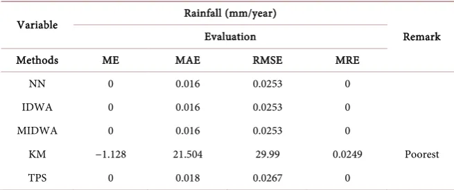
Even though the recommended radial distance for spatial interpolation is 100 km in most of the literature, it does not work effectively for this particularly identified study area due to complexity of the topography and sparse distribu-tion of meteorological stadistribu-tions over the study area. Therefore, in order to have the chance to compare the performance of all five methods of estimation for all four variables for the stations in consideration, the radius of influence was in-creased from 100 km to 200 km; and the result was pretty good in giving predic-tion results for all four variables involving all five methods of predicpredic-tion except rainfall at Addis Ababa-Bole station for the method TPS. As it can be seen from the results in Tables 4-7, the methods that estimated all variables very poorly is KM and the next poorest method is TPS. The remaining three methods (NN, IDWA, and MIDWA) are relatively performed best and these methods could be suggested to be applied for estimation of missing variables whenever necessary. When intercomparison was made method among the four variables (rainfall,

Table 5. Evaluation results for long-term average annual rainfall using ME, MAE, RMSE, and MRE.

Variable Rainfall (mm/year)

Remark Evaluation

Methods ME MAE RMSE MRE

NN 0 0.016 0.0253 0

IDWA 0 0.016 0.0253 0

MIDWA 0 0.016 0.0253 0

KM −1.128 21.504 29.99 0.0249 Poorest

Table 6. Evaluation results for long-term average wind speed using ME, MAE, RMSE, and MRE.

Variable Wind speed (km/hr)

Remark Evaluation

Methods ME MAE RMSE MRE

NN −0.029 0.031 0.0359 0.007

IDWA −0.193 0.195 0.457 0.033

MIDWA −0.233 0.235 0.5575 0.039

KM −0.022 0.294 0.524 0.0724 Poor

TPS 0.197 0.261 0.685 0.0401 Poor

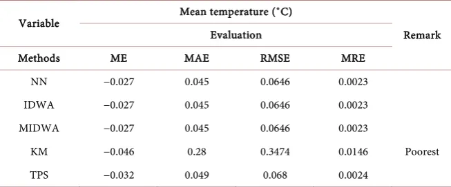
Table 7. Evaluation results for long-term mean temperature using ME, MAE, RMSE, and MRE.

Variable Mean temperature (˚C)

Remark Evaluation

Methods ME MAE RMSE MRE

NN −0.027 0.045 0.0646 0.0023

IDWA −0.027 0.045 0.0646 0.0023

MIDWA −0.027 0.045 0.0646 0.0023

KM −0.046 0.28 0.3474 0.0146 Poorest

TPS −0.032 0.049 0.068 0.0024

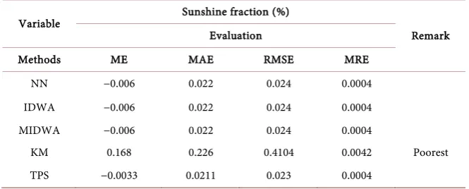
wind speed, mean temperature and sunshine fraction), it is very difficult to pre-dict wind speed using all methods as the errors are large relative to the remain-ing three variables. Therefore, it is not recommended to estimate missremain-ing values of wind speed using these evaluated methods, particularly for Diredawa station except NN method. The highest error recorded for KM is during estimation of rainfall, which shows that KM is not good method to be used for prediction of rainfall at some stations located in lowland areas like Dire Dawa, Gore, and Ne-gele except for Awash. But this method is found to be good at Addis Ababa-Bole, Debremarkos, Gondar, and Mekele stations. Relatively, Sunshine fraction and mean temperature were estimated in a good way using NN, IDWA, and MIDWA methods.

Generally, NN, IDWA, and MIDWA were best methods relative to the re-maining methods (KM and TPS) for all stations, except at Dire Dawa for estima-tion of wind speed using IDWA and MIDWA for both radial distances (r = 100 km and 200 km) for all variables. The summary of analysis result is summarized in Tables 5-8.

4. Conclusion

Table 8. Evaluation results for long-term mean sunshine fraction using ME, MAE, RMSE, and MRE.

Variable Sunshine fraction (%)

Remark Evaluation

Methods ME MAE RMSE MRE

NN −0.006 0.022 0.024 0.0004

IDWA −0.006 0.022 0.024 0.0004

MIDWA −0.006 0.022 0.024 0.0004

KM 0.168 0.226 0.4104 0.0042 Poorest

TPS −0.0033 0.0211 0.023 0.0004

MRE and RMSE) for estimation of four meteorological variables (rainfall, mean temperature, wind speed and sunshine fraction) over complex topography of Ethiopia by specifying radial distances of 100 km and 200 km. It was found that 100 km was not effective even though it is recommended in many kinds of lite-ratures. Hence, 200 km was selected for further analysis. The result of the analy-sis showed that KM and TPS methods are not good methods and NN, IDWA, and MIDWA methods are the best methods relatively. Estimation of rainfall in lowland areas like Diredawa, Gore, and Negele using KM is not good unlike that of Awash which has shown better results. When intercomparison is made among methods for the four variables (rainfall, wind speed, mean temperature, and sunshine fraction), it is very difficult to predict wind speed using all me-thods as the errors are large relative to the remaining three variables. This is also true for KM in predicting rainfall. Therefore, it is not recommended to estimate missing values of wind speed using these evaluated methods, particularly for Dire Dawa station except NN method. Mean temperature and sunshine fraction were estimated in a good way using NN, IDWA, and MIDWA methods.

Acknowledgements

I would like to thank my wife Etabezahu Tadese Belachew for her encouraging words and care during the unforgettable time of my life. This is not only my work but yours as well. Next, I appreciate the constructive suggestions give by the reviewer Wong Rui (Ray) from Journal of Water Resource and Protection (JWARP) editorial office.

Finally, this research did not receive any grant from funding agencies in the public, commercial or not-for-profit sectors.

References

[1] Presti, R.Lo., Barca, E. and Passarella, G. (2010) A Methodology for Treating Miss-ing Data Applied to Daily Rainfall Data in the Candelaro River Basin (Italy). Envi-ronmental Monitoring and Assessment, 160, 1-22.

https://doi.org/10.1007/s10661-008-0653-3

Meteor-ology, 96, 131-144.

[3] Caldera, H.P.G.M., Piyathisse, V.R.P.C. and Nandalal, K.D.W. (2016) A Compari-son of Methods of Estimating Missing Daily Rainfall Data. Engineer, XLIX, 1-8.

https://doi.org/10.4038/engineer.v49i4.7232

[4] Burhanuddin, S.N.Z.A., Denis, S.M. and Ramli, N.M. (2015) Geometric Median for Missing Rainfall Data Imputation. AIP Conference Proceedings, 1643.

https://doi.org/10.1063/1.4907433

[5] Villazón, M.F. and Willems, P. (2010) Filling Gaps and Daily Disaccumulation of Precipitation Data for Rainfall-Runoff Model. BALWOIS 2010, Ohrid, 25-29 May 2010.

[6] Wong, K.J., Fung, K.W. and Che, C. (2012) A Comparative Analysis of Soft Com-puting Techniques Used to Estimate Missing Precipitation Records. 2012 19th ITS Biennial Conference, Bangkok, 18-21 November 2012.

[7] Ramos-Calzado, P., Gomez-Camacho, J., Perez-Bernal, F. and Pita-Lopez, M.F. (2008) A Novel Approach to Precipitation Series Completion in Climatological Da-tasets: Application to Andalusia. International Journal of Climatology, 28, 1525- 1534. https://doi.org/10.1002/joc.1657

[8] Li, J. and Heap, A.D. (2008) A Review of Spatial Interpolation Methods for Envi-ronmental Scientists. Geosciences Australia, Record 2008/23, 137 p.

[9] Hijmans, R.J., Cameron, S.E., Parra, J.L. and Jones, P.G. (2005) Very High Resolu-tion Interpolated Climate Surfaces for Global Land Areas. International Journal of Climatology, 25, 1965-1978. https://doi.org/10.1002/joc.1276

[10] Jarvis, C.H. and Stuart, N. (2001) A Comparison among Strategies for Interpolating Maximum and Minimum Daily Air Temperatures. Part II: The Interaction between Numbers of Guiding Variables and the Type of Interpolation Method. Journal of Applied Meteorology, 40, 1075-1084.

https://doi.org/10.1175/1520-0450(2001)040<1075:ACASFI>2.0.CO;2

[11] Mardikis, M.G., Kalivas, D.P. and Kollias, V.J. (2005) Comparison of Interpolation Methods for Prediction of Reference Evapotranspiration—An Application in Greece. Water Resources Management, 19, 251-278.

https://doi.org/10.1007/s11269-005-3179-2

[12] Coulibaly, M. and Becker, S. (2007) Spatial Interpolation of Annual Precipitation in South Africa-Comparison and Evaluation of Methods. Journal of Water Interna-tional, 32, 494-502. https://doi.org/10.1080/02508060708692227

[13] Eklundh, L. and Pilesjo, P. (1990) Regionalization and Spatial Estimation of Ethio-pian Mean Annual Rainfall. International Journal of Climatology, 10, 473-494.

https://doi.org/10.1002/joc.3370100505

[14] Derib, S.D. and Diekkruger, B. (2011) Comparison of Spatial Interpolation Methods for Filling Daily Rainfall Missing Data, Blue Nile Basin, Ethiopia. Development on Margin, Bonn, 5-7 October 2011.

[15] Grieser, J., Gommes, R. and Bernardi, M. (2006) New Local Climate Estimator of FAO. Geophysical Research Abstracts, 8, Article ID: 08305.

[16] Awulachew, S.B., Yilma, A.D., Loulseged, M., Loiskandl, W., Ayana, M. and Alami-rew, T. (2007) Water Resources and Irrigation Development in Ethiopia. Interna-tional Water Management Institute, Colombo.

[17] Worldometeres (2016) Ethiopia Population.

http://www.worldometers.info/world population/ethiopia-population/

https://doi.org/10.1002/joc.1052

[19] Golkhatmi, N.S., Sanaeinejad, S.H., Ghahraman, B. and Pazhand, H.R. (2012) Ex-tended Modified Inverse Distance Method for Interpolation-Rainfall. International Journal of Engineering Inventions, 1, 57-65.

[20] Hutchinson, M.F. (1995) Interpolating Mean Rainfall Using Thin Plate Smoothing Splines. International Journal of Geographic Information Systems, 9, 385-403.

https://doi.org/10.1080/02693799508902045

[21] Apaydin, H., Sonmez, F.K. and Yildirim, Y.E. (2004) Spatial Interpolation Tech-niques for Climate Data in the GAP Region in Turkey. Climate Research, 28, 31-40.

https://doi.org/10.3354/cr028031

[22] Hutchinson, M.F., Mckenney, D.W., Lawrence, K., Pedlar, J.H., Hopkinson, R.F., Milewsha, E. and Papadopol, P. (2009) Development and Testing of Canada-Wide Interpolated Spatial Models of Daily Minimum-Maximum Temperature and Preci-pitation for 1961-2003. Journal of Applied Meteorology and Climatology, 48, 725- 741. https://doi.org/10.1175/2008JAMC1979.1

[23] Gomez, M.R.S. (2007) Spatial and Temporal Rainfall Gauge Data Analysis and Va-lidation with TRMM Microwave Radiometer Surface Rainfall Retrievals.Master’s Thesis,International Institute for Geo-Information Science and Earth Observation, Enschede.

[24] Wong, D.W., Yuan, L. and Perlin, S.A. (2004) Comparison of Spatial Interpolation Methods for the Estimation of Air Quality Data. Journal f Exposure Analysis and Environmental Epidemiology, 14, 404-415. https://doi.org/10.1038/sj.jea.7500338 [25] Stahl, K., Moore, R.D., Floyer, J.A., Asplin, M.G. and McKendry, I.G. (2006)

Com-parison of Approaches for Spatial Interpolation of Daily Air Temperature in a Large Region with Complex Topography and Highly Variable Station Density. Agricul-tural and Forest Meteorology, 139, 224-236.

https://doi.org/10.1016/j.agrformet.2006.07.004

[26] Thornton, P.E., Running, S.W. and White, M.A. (1997) Generating Surfaces of Dai-ly Meteorological Variables over Large Regions of Complex Terrain. Journal of hy-drology, 190, 214-251. https://doi.org/10.1016/S0022-1694(96)03128-9

Submit or recommend next manuscript to SCIRP and we will provide best service for you:

Accepting pre-submission inquiries through Email, Facebook, LinkedIn, Twitter, etc. A wide selection of journals (inclusive of 9 subjects, more than 200 journals)

Providing 24-hour high-quality service User-friendly online submission system Fair and swift peer-review system

Efficient typesetting and proofreading procedure

Display of the result of downloads and visits, as well as the number of cited articles Maximum dissemination of your research work