Munich Personal RePEc Archive
A control chart using copula-based
Markov chain models
Long, Ting-Hsuan and Emura, Takeshi
Graduate Institute of Statistics, National Central University, Taiwan
19 July 2014
Online at
https://mpra.ub.uni-muenchen.de/60346/
A control chart using copula-based Markov chain models
Long Ting-Hsuan, Takeshi Emura1
Graduate Institute of Statistics, National Central University, Taiwan
ABSTRACT
Statistical process control is an important and convenient tool to stabilize the quality of
manufactured goods and service operations. The traditional Shewhart control chart has been
used extensively for process control, which is valid under the independence assumption of
consecutive observations. In real world applications, there are many types of dependent
observations in which the traditional control chart cannot be used. In this paper, we propose to
apply a copula-based Markov chain to perform statistical process control for correlated
observations. In particular, we consider three methods to obtain the estimates of upper control
limit (UCL) and lower control limit (LCL) for the control chart. It is shown by simulations
that Joe’s parametric maximum likelihood method provides the most reliable estimates of the
UCL and LCL compared to the other methods. We also propose simulation techniques to
compute the average run length (ARL) of the proposed charts, which can be used to set the
UCL and LCL for a given value of ARL. The piston rings data are analyzed for illustration.
Keyword: Average run length, Clayton model, correlated data, Kendall’s tau, Markov chain.
JEL classifications: C13, C15, C18, C22
1 Corresponding author: Graduate Institute of Statistics, National Central University, Taiwan
1. Introduction
With the promotion of industrial technologies, statistical process control (SPC) has been
essential and convenient tools for manufacturers. Unavoidably, as factories produce items in
mass production, they encounter some defective items. The basic idea of SPC is to keep the
defective rate at some specified threshold (often at 0.27%). Consequently, the manufacturers
can control the loss of their business profits.
In the traditional Shewhart charts, the process measurements on items are assumed to be
independent. Unfortunately, the assumption of independence usually does not satisfy when the
intermission between samples is short. For instance, manufacturing ill-conditioned items
could cause machine's temperature to get higher than the normal condition. If the intermission
is short, the chance of producing ill-conditioned product in the next item increases. Hence,
very often in industrial practice, measurements are positively correlated.
A first order autoregressive AR(1), a first order moving average MA(1), and a first order
integrated moving average IMA(1) model are typically used for SPC with correlated
observations. A concise review of these models in the SPC literature is found in Box and
Narasimhan (2010). The early work starts with the papers by Johnson and Bagshaw (1974),
Bagshaw and Johnson (1975) and Vasilopoulos and Stamboulis (1978). After that, the
problem of SPC with correlated observation has been widely studied. A comprehensive
overview of this problem is found in Wieringa (1999), Knoth and Schmid (2004) and Psarakis
and Papaleonida (2007). Although higher order models are available, the literature on SPC
remains focused on the first order models (Wetherill and Brown 1991; Wardell, et al. 1994;
Wieringa, 1999; Knoth and Schmid, 2004; Psarakis and Papaleonida 2007; Montgomery
2009a, b; Box and Narasimhan, 2010). In this paper, we also consider a first order (i.e.,
Markov) model, but the dependence is modeled via copulas, which has not been considered in
2. Background
2.1 Copula-based Markov chain model
A copula is a bivariate distribution function with the two marginals being U(0,1).
Copulas are useful to model the dependence between the two random variables that are
transformed to U(0,1). Sklar (1959) showed that for any bivariate distribution function
) ,
(y1 y2
H with marginal distributions G1(y1) and G2(y2) , there exists a copula
] 1 , 0 [ ] 1 , 0 [
: 2
C such that
H(y1,y2)C(G1( y1),G2( y2)).
More information on copulas can be found in the books of Joe (1997) and Nelsen (2006).
Darsow, Nguten and Olsen (1992) first introduced copula-based Markov chain models
for serially correlated observations{Yt:t1,...,n}, where a copula defines the correlation
between Yt1 and Yt. The resultant series become a stationary process with the stationary
distribution G1G2 (Joe, 1997; Chen and Fan, 2006). The copula-based Markov model
includes the 1st order autoregressive model, or AR(1), as a special case with a Gaussian copula
and normal margin (p.260 of Joe, 1997).
This paper focuses on the one-parameter Clayton copula defined as:
) 0 1 (
) 1 (
) ; ,
( 1 2
/ 1 2
1 2
1
u u u u
u u
C I ,
where (1,)\{0} describe the correlation between Yt1 and Yt. If (1,0),
1
t
Y and Yt have negative correlation; when (0,) , Yt1 and Yt have positive
correlation. It is well known that the correlation measure on the scale of [-1, 1] is represented
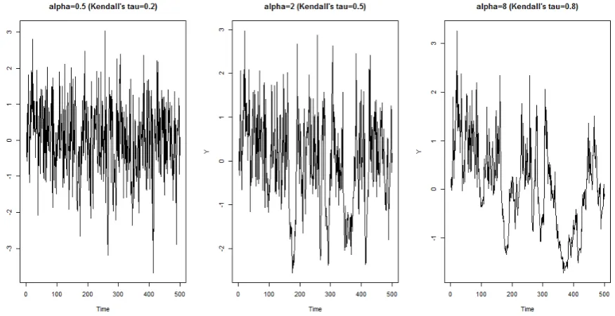
by Kendall's tau /(2). Figure 1 shows the plot of the first-order Markov series
} ..., , 1 :
{Yt t n under the Clayton copula with the marginal being the standard normal
Fig. 1. The plot of {Yt:t1,...,n} under the Clayton copula with the marginal being the
standard normal distribution, where n500.
In this article, we focus on the Clayton copula due to its popularity in applications. Some
recent applications of the Clayton copula are referred to Sari et al. (2009) for industrial
statistics and Emura and Chen (2014) for biostatistics.
2.2 Motivation and the organization
In this paper, we assume that only one observation is available at each time, as usually
assumed in the literature of SPC for autocorrelated data (Schmid, 1995; Wieringa, 1999;
Kramer and Schmid, 2000; Knoth and Schmid, 2004; Psarakis and Papaleonida, 2007; Box
and Narasimhan, 2010; Hryniewicz, 2012). Hence, we monitor individual observations
} ..., , 1 :
{Yt t n rather than subgroup averages. This is because the serial correlation reduces
by taking subgroup averages (Wieringa, 1999).
The main theme of this paper is the application of the copula-based Markov chain
control limit (LCL) for {Yt:t1,...,n}. If the marginal mean and the marginal standard
deviation of Yt are known, one may set the three-sigma limits LCL=3 and UCL=
3 . For the aforementioned example of the Clayton model with the standard normal
margins ( 0, 1), the UCL and LCL are +3 and -3, respectively.
In many real examples, such theoretical limits are unknown since the marginal
distributions ( and ) are unknown. Therefore, the control limits must be estimated using
the in-control data or Phase I data (p.230 of Montgomery 2009a). To the best of our
knowledge, there is no paper discussing the estimation of the control limits under the
copula-based time series models. Therefore, the primary objective of this paper is developing
estimation procedures for ULC and LCL, which is detailed in Section 3. Then, Section 4
contains simulations that investigate the performance of the methods in Section 3.
If observations are correlated, however, the above three-sigma limits
3
may notkeep the average run length (ARL) at the desired level (often at ARL=370). In the case of
dependent observation, one might alternatively determine the UCL and LCL such that the
ARL is equal to a given value. This is done by selecting a constant c such that the limits
c achieve a given ARL (Schmid, 1995). Besides setting the control limits, the ARL isan important measure of the performance of a control chart. Therefore, the secondary
objective of this paper is developing appropriate simulation techniques for calculating the
ARL under a copula-based Markov model, which is detailed in Section 5. The choice of c
will be discussed with the real data analysis in Section 6.
Chapter 7 concludes the paper. Detailed calculations are given in Appendices.
3. Estimation of process parameters
We introduce methods to estimate parameters that are useful for SPC. Such parameters
3.1. Model assumptions
Following Joe (1997) and Chen and Fan (2006), we impose the following assumption
throughout the paper:
Assumption 1
Let {Yt :t1,...,n} be a sequence of random variables, representing a quality
characteristics. The variables follow a stationary first-order Markov process with the
transition probability determined by
) ); ( ), ( ( ) , ( )
,
( 1 * *
* 1
* 1
1 t t t t t t t
t y Y y H y y C G y G y
Y
P ,
where *()
G is continuous marginal (stationary) distribution and (,;*)
C is the true
parametric copula for an unknown value *. Assume that, the copula is also continuous, and
is neither the Fréchet–Hoeffding upper nor lower bound.
Assumption 1 derives the conditional density of and Yt given Yt1 via
( ) ( ( ), *( ); * )
1 *
*
t t
t c G y G y
y
g ,
where (,;*)
c is the copula density of (,;*)
C , and *()
g is the density of the true
marginal (stationary) distribution *()
G .
Under Assumption 1, the transformed process, { : *( )}
t t
t U G Y
U is a stationary
Markov process of order 1 in which the joint distribution of Ut and Ut1 is given by the
copula ( , ; *)
1 0 u
u
C , and the conditional density of Ut given Ut1u0 is
) ; , ( )
( 0 *
| 1 0 u c u u
fUtUtu . This property is shown to be useful for generating the data.
3.2. Joe’s method
We demonstrate how the likelihood estimator of Joe (Joe, 1997) can be used to estimate
relevant parameters. In most quality control work, relevant parameters are E(Yt ) and
) var(Yt
to get the control limits 3. Hence, it is convenient to parameterize *
in terms of (, ). Here we propose to set G*(y){(y)/}, where is the
distribution function of N(0,1).
The log-likelihood function given data {yt:t1,...,n} is
n
t
t t
n
t
t y y
c n
y n
L
2
1
1
; ,
log 1 1
log 1 ) , ,
(
.
The formula of log-copula density logc(u1,u2;) is given in Appendix A.1. The maximum
likelihood estimator (MLE) that maximizes the preceding formula is denoted by (ˆ,ˆ,ˆ ).
The resultant estimators of LCL and UCL are ˆ3ˆ and ˆ3ˆ, respectively.
The log-likelihood function L(,,) is twice differentiable and the formulas of the
first and second derivatives are given in Appendix A.2. The derivatives are quite complicated
but they are useful for likelihood inference.
It is well-known that the Newton-Raphson algorithm is sensitive to the initial values,
especially in estimating three or more parameters (see Section 5.7 of Knight (2000)). We also
encounter the cases that the algorithm diverges due to a wrong initial value. Knight (2000)
suggests trying several different initial values. Based on this suggestion and our own
numerical experiences, we propose the following “randomized” Newton-Raphson algorithm:
Newton-Raphson algorithm with randomization
Step 1: Choose the initial value (0,0,0 ), defined as
n
t t
Y n Y
1 0
1
, 2
1 2
0 Y /n Y
n
t
t
, 0 20/(01),
where
j i
i j i
j Y Y Y
Y n
} ) (
sgn ) (
sgn {
2 1 1
1
0
,
and where sgn( x)1 for x0, sgn(x)0 for x0 and sgn(x)1 for x0.
Set ) , , ( ) , , ( 1 2 2 2 2 2 2 2 2 2 1 1 1 k k k k k k L L L L L L L L L L L L k k k k k k
for k 0,1,..., where the formulas for the derivatives are given in Appendix A.2.
If 5
1 5
1 5
1 | 10 ,| | 10 and | | 10
|k k k k k k , stop the algorithm and set
) , , ( ) ˆ , ˆ , ˆ
( k1 k1 k1 .
If 1 20
20 1
20
1 | 10 , | | 10 or | | 10
|k k k k k k , replace (0,0,0) with
) ,
,
(0 0 0u , where u~unif(0.1,0.1), and return to Step 1.
Recently, Hu (2014) successfully applied a similar randomized Newton-Raphson method
to stabilize the computation of the MLE under double-truncation. The estimators for the LCL
and UCL are ˆ3ˆ and ˆ3ˆ, respectively.
3.3. Chen and Fan’s method
Chen and Fan (2006) proposed a copula-based Markov chain to describe the dependence
structure for financial time-series data. In their paper, they considered a semi-parametric
copula model with non-parametric marginal distributions. In this section, we discuss how to
apply their method to estimate relevant parameters that are useful for SPC.
The semi-parametric copula-based Markov chain model has unknown parameters
) ,
(G* * . Chen and Fan (2006) proposed to estimate the unknown marginal (stationary)
distribution G* using Gn(), the rescaled empirical distribution function defined as
n t tn Y y
n y G 1 } { 1 1 )
( Ι .
can use the Stieltjes integral to get the estimators
, 1 )
(
ˆ Y
n n y
ydGn
where
n
t t n
Y Y
1
/ , and
.
1 1
1 ] ) ( [
) (
ˆ
2
1 2 2
2 2
Y n
n Y
n y
y d G y
dG y
n
t t n
n
Hence,
.
1 1
1
ˆ
2
1 2
Y n
n Y
n
n
t t
If the marginal distribution G*() is known, then the log-likelihood function is given by
n
t
n
t
t t
t c G Y G Y
n Y g n
L
1 2
* 1 * *
) ); ( ), ( ( log 1 ) ( log 1 )
( .
Then, the unknown *
is estimated by maximizing the above function with G*() being
replaced by Gn(). The estimators for LCL and UCL are ˆ3ˆ and ˆ3ˆ, respectively.
3.4. Standard method
It is of interest to compare the above two methods with the standard estimators defined as
n
t t
Y n Y
1
1
ˆ
,
21 2
1
ˆ Y Y
n
n
t
t
.
The corresponding estimators for the LCL and UCL are ˆ3ˆ and ˆ3ˆ, respectively.
Such estimators were considered in Kramer and Schmit (2000) under AR(1) models. The
standard estimator is consistent but may incur the loss of efficiency by ignoring correlation.
4. Simulations
We have introduced three methods to estimate the process parameters. To know which method
4.1. Simulation methods
We develop the algorithm for generating {Yt:t1,...,n} by extending the conditional
approach for bivariate copula models (Frees and Valdez, 1998). Our simulations focus on the
Clayton copula with 2( 0.5) , 8( 0.8) and 1/3( 0.2) . We
choose the marginal (stationary) distribution to be the normal distribution
} / ) ( { ) (
*
y y
G with (, )=(1,1). The algorithm is stated as follows:
Algorithm 1 ( Data generation )
1. Generate a random number U1, where U1~unif(0,1). Then, set ( 1)
1
1 U
Y , where
} / ) ( { )
(
y y .
2. Set {[1 ( /( 1) 1) ( ) ] 1/ }
1 1
1
t t
t U Y
Y , where Ut1~unif(0,1), t1,...,n.
After generating the data, we calculate parameter estimates using the three methods:
Method 1 ( Joe’s method; see Section 3.2 )
Method 2 ( Chen and Fan’s method; see Section 3.3 )
Method 3 ( Standard method; see Section 3.4 )
The MSE of an estimator ˆ with respect to the unknown parameter is defined as
] )
ˆ
( E[ )
ˆ
MSE( 2
. We compare the three methods in terms of the MSE for , ,
and 3 . We also examine the bias, defined as Bias(ˆ)E(ˆ).
4.2. Simulation results
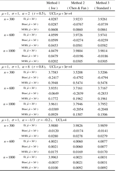
The results based on 1000 repetitions are given in Tables 1-3. Generally speaking, the
three methods give estimates ˆ close to the true values of , and 3 ,
Under positive correlation ( 0), it is clear that the MSE for Joe’s method is always
smaller than other two methods (Tables 1-3). Under 2 ( 0.5), Joe’s method reduces
)
ˆ
MSE( and MSE(ˆ 3ˆ ) about by half the MSEs for the other two methods. When
8
( 0.8), Joe’s method gives remarkably superior MSE(ˆ3ˆ ) to the other
methods. The dominance of Joe’s method over the other two becomes modest in terms of
)
ˆ
MSE( . In SPC, however, the accuracy of MSE(ˆ3ˆ ) is more important than
)
ˆ
MSE( since the out-of-control signals are decided by the UCL and LCL.
Under negative correlation (0), the three methods are quite comparable. The MSE of
the three methods are very similar for all configurations. Overall, the MSE under the negative
correlation is much smaller than that under positive correlation.
The efficiency of Joe’s method is reasonable since it is performed under the correct
assumptions on the Clayton copula and the normality. On the other hand, Chen and Fan’s
method and standard method do not rely on the distributional assumptions. To see the
performance under a model misspecification, we generate heavy-tailed data {Yt*:t1,...,n}
under the t-distribution by
] }; / ) ( { [
2 1
*
t
t Y
Y ,
where 1[; ] is the quantile function of the t-distribution with degree of freedom 10.
The performance of the three methods are comapred in Table 4. Although Joe’s method is still
the best for all configurations, its superiority becomes somewhat offset.
Therefore, as long as the true model is correctly specified or approximated well, Joe’s
method is most accurate in terms of MSE under positively correlated series. Since industrial
settings typically faces with positively correlated series, Joe’s method seems to be of great
5. Average run length
In this section, we develop simulation techniques to obtain the average run length (ARL).
In particular, we choose the antithetic variables method to gain computational efficiency.
5.1. Calculation of ARL
The average run length (ARL) of a control chart is one way to determine the
performance of control charts. The ARL is the average number of sample points that are
plotted before a point is beyond the control limits. The ARL can help engineers know the
performance of chart under study. For instance, if the process is in-control, engineers wish to
keep the production process as long as possible. Hence, the chart that has a large ARL is
preferred. The ARL is defined as follows:
Definition (ARL):
Let {Yt,t1,2,...} be a sequence of random variables, representing a quality
characteristics and Amin{t:Yt 3 orYt 3} be the run length. Then, the
ARL is defined to be E( A).
If {Yt,t1,2,...} are independent and identically distributed, the ARL is easily
calculated as E( A)1/p , where pP(Y1 3 orY1 3) [see p.37 of
Wieringa (1999); p. 249 of Montgomery (2009a)]. However, for correlated observations, the
ARL calculation is extremely difficult. Schmid (1995) proposed some analytical methods to
calculate the ARL. However, his formula is complicated and does not give us practical way to
calculate the ARL. Schmid (1995) and Hryniewicz (2012) used Monte Carlo simulations to
calculate the ARL under the autoregressive model and copula-based chain model, respectively.
copula-based models.
One can use Algorithm 1 to generate data until the data falls outside control limits and
then obtain the value of run length. Repeating this step many times, we get the ARL. In this
paper, we set m = 10000 repetitions. The algorithm is as follows:
Algorithm 2 ( ARL with Monte Carlo )
1. Draw Y1 ~ N(, ).
2. Draw Ut1 ~unif(0,1), and then set {[1 ( /( 1) 1) ( ) ] 1/ }
1 1
1
t t
t U Y
Y
for t1,2,..., where (y){(y)/}.
3. Calculate the run length Amin{t:Yt 3 or Yt 3}.
4. Repeat Step 1 ~ Step 3 m times. The ARL is the average of the m run length.
5.2. Antithetic variables
The calculation of the ARL requires a large number of Monte Carlo runs to get an
accurate result. Some simulation techniques can help reduce the computational cost. The
well-known techniques are common random number, antithetic variables, control variates,
stratified sampling and important sampling (Chapter 9, Ross, 2013). We introduce antithetic
variables method, which is a simple method to reduce variable and computational cost.
The antithetic variables method aims to reduce the variance by introducing correlation in
the series of Monte Carlo runs. In Algorithm 2, the ARL is written as Ah{Ut;t1,2,...}. It
is important to notice that Bh{1Ut;t1,2,...} has the same distribution as A. This
implies that (AB)/2 is unbiased for the ARL. Furthermore, if cov( A,B)0, then
2 / ] var[ ] 2 / ) (
var[ AB A .
which becomed smaller than the variance of the average of two independent sequences. The
Algorithm 3 ( ARL with antithetic variables )
1. Draw Y1 ~ N(, ).
2. Draw U1 ~unif(0,1) and then set ( 1)
1 1 ,
1 U
Y and 1(1 1 )
1 ,
2 U
Y , where
} / ) ( { )
(
y y .
3. Draw Ut1~unif(0,1) and set {[1 ( 1) ( 1, ) ]1/ }
) 1 /( 1 1
1 , 1
t t
t U Y
Y , t 1,2,...
4. Calculate Amin{t:Y1,t 3 orY1,t 3}.
5. Set {[1 ((1 ) 1) ( ) ]1/ }, 1,2,...
, 2 )
1 /( 1 1
1 ,
2
U Y t
Y t t t .
6. Calculate Bmin{t:Y2,t 3 orY2,t 3}.
7. Repeat step 1~step 6 m times, and get two sequences (A1,...,Am ) and (B1,...,Bm ). The
ARL is
im1(AiBi )/2m.Remark: In Step 3 and Step 5, we use common uniform random variables. In this way, we
save the number of generating uniform random numbers by half, compared with Algorithm 2.
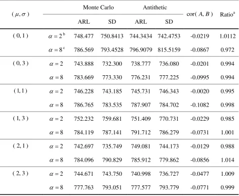
5.3. Simulation results
We compare the calculation of the ARL between the Monte Carlo method (Algorithm 2)
and antithetic variables method (Algorithm 3) under the same simulation settings as Section
4.1. To check whether the use of antithetic variables reduces the variance or not, we compare
the standard deviation (SD) of the antithetic variables method with that of the usual Monte
Carlo method. For the two algorithms to be comparable, the ARL for the Monte Carlo is
) 2 /(
2 1
m
i Ai m and for the anntithetic variables method is
m
i 1( Ai Bi)/(2m), where m =
10000. Thus, the SD for the Monte Carlo method is
21 2/(2 ){
i2m1 i/(2 )}2m
i Ai m A m
and for the antithetic variables method is
1( 2 2 )/(2 ){
im1( i i )/(2 )}2m
Smaller SD corresponds to better computational efficiency. We also calculate the sample
correlation between the two sequences of the antithetic variables, denoted by cor( A,B). If
0 ) , (
cor A B , we expect that the antithetic variables method reduces the SD.
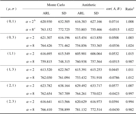
The results are given in Table 5. The Monte Carlo and antithetic variables methods
produce similar values for the ARL, which means that the two methods give a good
approximation to the true ARL. Also, the SD of the two methods is quite similar. This implies
that the variance reduction using the antithetic variables is quite modest. This result agrees
with the fact that cor( A,B) is very close to zero. However, it should be noted that the
antithetic variables method reduces by half the number of generating random numbers.
We also examine the case of the one-sided control limit in which the ARL is the average
number of sample points that are plotted before a point is beyond the UCL only, i.e.
} 3 :
min{
t Yt
A . The results are summarized Table 6. In this case, cor( A,B)0
occurs in all configurations. The reason is that, if the sequence A reaches the UCL, the
alternative sequence B gets close to the LCL. However, the effect of negative correlation is
modest and there is no apparent efficiency gain. In conclusion, the antithetic variables method
saves the number of random samples but does not improve efficiency.
We display the properties of both in-control and out-of-control ARL under various
Kendall’s tau in Table 7. It is seen that the ARL increases as Kendall’s tau increases. This
kind of the increase of the ARL with the correlation is well known (e.g., Schmid, 1995;
Wieringa, 1999; Konth and Schmid 2004), and is in accordance with the simulation results of
Hryniewicz (2012). The out-of-control ARL (1 -shift or 2 -shift) is substantially smaller
than the in-control ARL, showing the good performance in detecting the out-of-control state.
However, when the correlation is large, there is some delay in detecting the out-of-control
signals. Under the case that Kendall’s tau=0.0001, the ARL values agree with the well-known
ARL values of the Shewhart chart for independent observations (ARL=370 under in-control;
To keep the in-control ARL at desired level (e.g., 370), one can select constant c such
that the limits
c
achieve a given ARL (Schmid, 1995). To do this, one can try manydifferent values of c to calculate the ARL using either Algorithm 2 or 3. Then, the appropriate
value of c is the one that is closest to the desired ARL. This procedure will be explained in the
subsequent real data analysis. Obviously, this is a computationally intensive procedure. As the
future work, we wish to reduce the computational cost by importance sampling [see Chen,
Fuh, and Teng (2013) and reference therein]. However, this is challenging since the definition
of the ARL involves infinitely many random variables.
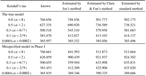
5.4. ARL under estimated parameters
If the marginal mean and the marginal standard deviation are unknown, one
needs to estimate them from data under in-control status, which is often done in Phase I trial
(Montgomery, 2009a). These estimates are used to calculate the UCL and LCL to set the
control limit of Phase II. Here, the primary interest is to find a good estimator that have small
deviation from the specified in-control ARL (true ARL). We conduct simulations to
investigate the influence of parameter estimation on the ARL of Phase II. Such simulation
designs have been considered in Kramer and Schmid (2000) and Hryniewicz (2012).
Table 8 compares the ARL under the estimated parameters and the true ARL, where the
true ARL represents the case of the known UCL and LCL. For estimated parameters, the UCL
and LCL have random variation due to estimation in Phase I. We use the three methods (Joe’s
method, Chen and Fan’s method and standard method) to estimate the UCL and LCL. Table
8 shows that the standard method leads to the ARL that are somewhat different from the true
ARL. This is because the standard method provides less accurate estimate of the UCL and
LCL, especially for strongly correlated cases. Although this is pointed out by Hryniewicz
(2012), the paper does not offer the solution. Similarly, Chen and Fan (2006) also performed
the correlation is high (Kendall’s tau = 0.8), only Joe’s method give reasonable approximation
to the true ARL.
Based on the fact that Joe’s method relies on the normality assumption, we also conduct
simulations under model misspecifications. Table 8 shows the results under misspecification
in Phase I, based on the t-distribution with degree of freedom 10 (as considered in
Section 4.2). Although Joe’s method still provides the best approximation to the true ARL, the
advantage is reduced. Therefore, as long as the normality assumption is approximated well,
Joe’s method would be recommended.
6. Data analysis
We demonstrate the proposed copula-based control chart using the data on diameter
measurements of piston rings (Montgomery, 2009b). We download the data available from R
qcc package (Luca, 2014), and obtained the diameter measurements {Yt;t1,2,...,200} for
the 200 samples.
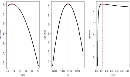
Using Joe’s method, the estimates are obtained as ˆ = 74.0036, ˆ = 0.0115, and ˆ
= 0.1422 that corresponds to Kendall’s tau = 0.0664. Therefore, the data exhibit weak positive
dependence. In the last step of the Newton-Raphson algorithm, we examine the gradient
-9 -9 -11
)
ˆ
,
ˆ
,
ˆ
(
10 2.248266 10
2.072281 10
1.517216
-
L L L
,
and the Hessian matrix
0.4012899
-26.60758 3.277339
-26.6075763 1
15025.2185
-646.070688
-3.2773394
-646.07069
-9 6108.55532
-)
ˆ
,
ˆ
,
ˆ
( 2 2
2
2 2
2
2 2
2
L L
L
L L
L
L L
L
.
)
ˆ
,
ˆ
,
ˆ
( is a local maxima. We have confirmed the global uniqueness of the MLE by
[image:19.595.91.529.149.407.2]drawing the likelihood functions. Figure 2 shows that ( ˆ,ˆ,ˆ ) attains the maximum.
Fig. 2. The likelihood function for the piston rings data (Montgomery 2009b).
The vertical line signifies the MLE ˆ = 0.1422, ˆ =74.0036, and ˆ = 0.0115.
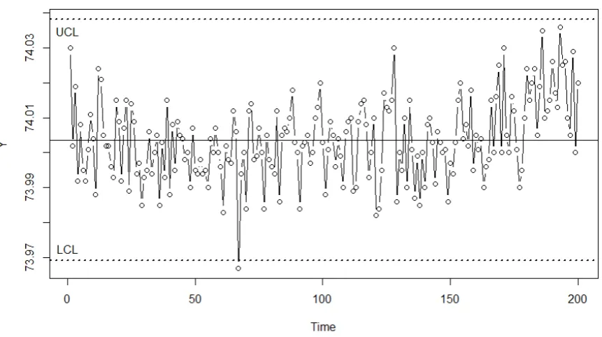
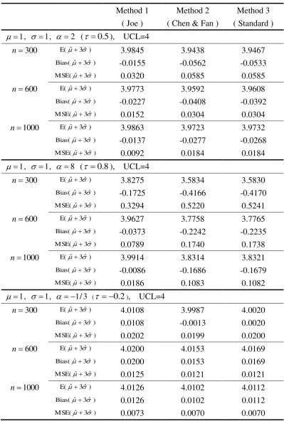
The resultant control chart is displayed in Figure 3. The MLE produces UCL (ˆ3ˆ ) =
74.0381 and LCL (ˆ3ˆ ) = 73.9691. Only one point, corresponding to the 67th observation,
gives the out-of-control signal, and all the others fall between LCL and UCL. Therefore, some
Fig. 3. The control chart using the piston rings data (Montgomery 2009b).
The center line represents the estimated mean ˆ, and the other two straight lines are UCL
(ˆ3ˆ) and LCL (ˆ3ˆ ), which are obtained by Joe’s method under the Clayton copula.
Under the estimated parameters, we calculate the ARL under the Clayton copula with
= 0.1535 and the normal distribution with =74.0036 and = 0.0115. Here, the 3-sigma
limits are UCL (3) = 74.0381 and LCL (3) =73.9691. Using Algorithm 2 (Monte
Carlo) with m = 10000, we obtain the ARL = 382.442 (se = 3.885). Suppose that one wishes
to have a control chart with ARL = 370. Accordingly, we reduce the coefficient from 3 to 2.99.
Then, the choice UCL (2.99) = 74.0380 and LCL (2.99 ) = 73.9693 achieves the
desired ARL = 371.155 (se = 3.767).
7. Conclusion and discussion
This paper provides a framework for performing statistical process control using
utilized to many different fields, the application to statistical process control has not been
considered in the literature. In particular, we demonstrate how to apply Joe’s method, Chen
and Fan’s method, and the standard method for calculating the control limits, and then
compare their performance via simulations. The results show that Joe’s method performs best
in terms of accuracy of the estimated control limits and the average run length with estimated
parameters, when the model assumptions are adequate. Hence we propose to use Joe’s method
for the application to statistical process control. For illustration, we demonstrate the usage of
Joe’s method for diameter measurements of piston rings data.
We also propose simulation techniques to calculate the average run length of the
proposed control charts. The Monte Carlo method and antithetic variables method are
presented, where the latter reduces by half the number of generating uniform random numbers.
It is demonstrated through the data analysis that the algorithms are useful when one wishes to
set copula-based control limits for a given value of the average run length.
Although we have applied a copula-based Markov model for a serially correlated data,
there are many cases where two series of correlated data are available. Specifically, suppose
that one observe two quality characteristics, say {Xt:t1,...,n} and {Yt:t1,...,n}. If there
is no serial correlation within each series, the correlation between the two series is modeled
by a bivariate normal distribution. Then, the simultaneous monitoring of the two series is
performed by a control ellipse or Hotelling 2
T -chart (Chap.11 of Montgomery, 2009a).
These approaches must be modified to take into account serial correlation in the two series. In
the presence of two series, one is not only interested in monitoring the process mean, but also
the association between the two series. For instance, the inner diameter Xt may change the
outer diameter Yt of some parts. Such monitoring schemes have not been considered in the
SPC context, but there are a rich literature studying on the causal relationship between two
series. We only mention that many methods to study the causal relationship between the series
The extension of the copula-based process control to the discrete variables is an
important direction for future research. Due to Assumption I, the method presented in this
paper is only applicable to continuous margins. However, the well-known np-control chart
and c-control chart assume that the observations follow independent binomial distribution and
Poisson distribution, respectively (Wetherill and Brown 1991; Montgomery 2009a, b). The
copula approach to incorporate the dependence is a challenging but interesting topic since
estimation under the copula models with discrete margins are relatively new. The difficulty
comes from the fact that the correlation parameter for copula models may be affected by the
marginal distributions [see Nešlehová (2007) for binomial margins and Genest, Nešlehová
and Rémillard (2013) for Poisson margins]. Another challenge in the np-control chart is that it
requires large n and not too small p (Emura and Lin, 2013). The copula approach to the
discrete cases will be a promising topic for research.
One of important issues that we did not discuss in this paper is the goodness-of-fit of a
given copula. We choose the Clayton copula for its popularity in applications and
mathematical tractability. Obviously, there are many other choices, such as Frank, Gumbel,
Gaussian copulas (Nelsen, 2006). Many of the goodness-of-fit methods for parametric models
use distance statistics, such as the Kolmogorov-Smirnov statistic and Cramér-von Mises
statistic. The asymptotic distribution of such statistics under the null model typically requires
the empirical process techniques (Genest, Rémillard, and Beaudoin, 2009; Emura and Konno,
2012), which needs further study.
Acknowledgments
We would like to thank the editor, associate editor and two anonymous reviewers for their
helpful comments that greatly improved the manuscript. This work was financially supported
References
Bagshow, M., Johnson, R. A. (1975). The effect of serial correlation on the performance of CUSUM tests II.
Technometrics 17, 73-80.
Box, G., Narasimhan, S. (2010), Rethinking statistics for quality control. Quality Engineering 22, 60-72.
Chen, X., Fan, Y. (2006). Estimation of copula-based semiparametric time series models. Journal of
Econometrics 130, 307-335.
Chen, C. C., Fuh, C. D. and Teng, H. W. (2013). Efficient option pricing with importance sampling. Journal of
the Chinese Statistical Association 51, 253–273
Darsow, W. F., Nguten B., Olsen, E. T. (1992). Copulas and Markov Processes. Illinois Journal of Mathematics
36, 600-642.
Emura, T., Konno, Y. (2012). A goodness-of-fit tests for parametric models based on dependently truncated data.
Computational Statistics & Data Analysis 56, 2237-2250.
Emura, T. and Chen, Y.H. (2014), Gene selection for survival data under dependent censoring: a copula-based
approach, Statistical Methods in Medical Research, doi: 10.1177/0962280214533378.
Emura T., Lin Y. S. (2013), A comparison of normal approximation rules for attribute control charts. Quality and
Reliability Engineering International, doi: 10.1002/qre.1601.
Frees, E. W., Valdez, E. (1998). Understanding the relationships using copulas. North American Actuarial
Journal 2, 1-25.
Genest, C., Rémillard, B. (2008). Validity of the parametric bootstrap for goodness-of-fit testing in
semiparametric models. Annales de Institut Henri Poicare -Probabilites et Statistiques 44, 1096-1127.
Genest, C., Nešlehová, J.G., Rémillard, B. (2013). On the estimation of Spearman’s rho and related tests of
independence for possibly discontinuous multivariate data. Journal of Multivariate Analysis 117, 217-228.
Hung, Y. C., Tseng, N. F. 2013. Extracting informative variables in the validation of two-group causal
relationship. Computational Statistics 28, 1151-1167.
Hu, Y. H. (2014). Maximum likelihood estimation for double-truncation data under a special exponential family,
Master Thesis, Graduate Institute of Statistics, National Central University, Taiwan.
Hryniewicz, O. (2012). On the robustness of the Shewhart control chart to different types of dependencies in
data. Frontiers in Statistical Quality Control 10, Lenz, H.-J. et al. (Eds.), Springer-Verlag Berlin Heidelberg.
Joe, H. (1997). Multivariate Models and Dependence Concepts. CHAPMAN & HALL/CRC.
Johnson, R. A., Bagshaw, M. (1974). The effect of serial correlation on the performance of CUSUM tests.
Technometrics 16, 103-112.
Knight, K. (2000). Mathematical Statistics. Chapman & Hall.
Knoth, S., Schmid, W. (2004). Control charts for time series: a review. Frontiers in Statistical Quality Control 7,
Lenz, H.-J. et al. (Eds.), Springer-Verlag Berlin Heidelberg.
Kramer, H. G., Schmid, W. (2000). The influence of parameter estimation on the ARL of Shewhart type charts
for time series. Statistical Papers 41, 173-196.
Montgomery, D. C. (2009b). Introduction to Statistical Quality Control, Sixth Edition. Wiley.
Nelsen, R. B. (2006). An Introduction to Copulas, 2nd Edition. Springer Series in Statistics, Springer-Verlag.
New York.
Nešlehová, J. (2007). On rank correlation measures for non-continuous random variables, Journal of Multivariate Analysis 98, 544-567.
Psarakis, S., Papaleonida, G. E. A. (2007). SPC procedures for monitoring autocorrelated processes, Quality
Techinology & Quantitative Management 4 (4), 501-540.
Ross, S. M. (2013). Simulation, Fifth Edition. Elsevier.
Sari, J. K., Newby, M. J., Brombacher, A. C., and Tang, L. C. (2009), Bivariate constant stress degradation model:
led lighting system reliability estimation with two-stage monitoring, Quality and Reliability Engineering
International 25, 1067-1084.
Schmid, W. (1995). On the run length of a Shewhart chart for correlated data. Statistical Papers 36, 111-130.
Sklar, A. (1959). Fonctions de re'partition a' n dimensions et leurs marges. Publications de l'Intitut de Statistique
de l'Universit de Paris 8, 229-231.
Vasilopoulos, A. V., Stamboulis, A. P. (1978), Modification of control chart limits in the presence of data
correlation. J. Quality Technology 10 (1), 20-30.
Wardell, D. G., Moskowitz, H, Plante, R. D. (1994). Run-length distributions of special-cause control charts for
correlated process. Technometrics 36, 3-27.
Wetherill G. B., Brown D. W. (1991) Statistical process control, theory and practice. Chapman and Hall.
Wieringa, J. E. (1999) Statistical process control for serially correlated data, Labyrint Publishing.
Appendices
A.1 Log-density for the Clayton copula
The density of the Clayton copula is given by
) 2 ( 2 1 ) 1 ( 2 ) 1 ( 1 2
1 2
1 2 2
1
1
] 1 [
) 1 ( /
) ; , ( ) ; ,
c(u u C u u uu u u u u , 0.
Hence, the log-copula density is:
) 1 log(
2 1 log
) 1 ( log ) 1 ( ) 1 log( ) ; ,
( 1 2 1 2 1 2
u u u u
u u
l .
A.2 Likelihood function and its first and second derivatives
Let ut1{(Yt1)/ } and Ut1{(Yt1)/ }. Using the formulas of Appendix
. ) 1 log( 2 1 log ) 1 ( log ) 1 ( ) 1 log( 1 2 ) ( 1 log ) 2 log( 2 1 ) , , ( 2 1 1 1 2 2
n t t t t t n t t U U U U n Y n L Hence, its derivatives are
nt t t
t t t t t t t t n t t U U u U u U U u U u n Y n L 2 1 ) 1 ( 1 ) 1 ( 1 1 1 1 2 , 1 1 2 1 1 1 ) , , (
nt t t
t t t t t t n t t t t t t t n t t U U u U Y u U Y n U u Y U u Y n Y n L 2 1 ) 1 ( 2 1 ) 1 ( 1 2 1 2 2 1 1 2 1 1 3 2 , 1 } / ) ( { } / ) ( { ) 2 1 ( 1 ) 1 ( 1 1 ) ( 1 ) , , ( , 1 log log 1 2 1 ) 1 log( ) log( 1 1 1 ) , , ( 2 1 1 1 2 2 1 1
nt t t
t t t t n t t t t t U U U U U U n U U U U n L , ) ( ) 1 ( ) 1 ( 2 1 1 / } / ) ( { / } / ) ( { 1 1 1 ) , , ( 2 2 ) 1 ( 1 ) 1 ( 1 1 1 2 1 2 2 2 2 2 1 2 1 1 1 2 1 2 2 2
n t t t t t t t t t n t t t t t t t t t t t u U u U U U H U U n U u u U Y U u u U Y n L where t t t t t t t t tt U u
Y u U u U Y u U
, ) 1 ( ) 1 ( ) 2 1 ( 1 ) ( 2 ) 1 ( 1 ) ( 2 ) 1 ( 1 1 ) ( 3 1 ) , , ( 2 2 1 1 2 1 2 2 2 3 2 1 1 1 2 2 1 1 1 3 1 1 2 4 2 2 2
n t t t t t n t t t t t t t t n t t t t t t t t n t t K U U K U U n U u Y Y U u Y n U u Y Y U u Y n Y n L where , ) 1 ( 2 ) 1 ( 2 2 ) 1 ( 3 2 1 1 1 1 1 ) 1 ( 1 3 1 1 t t t t t t t t t t t t t t Y Y U u u U Y Y Y U u u U Y Kand {( )/ }{ 1 (1 ) }
) 1 ( 1 2 1
2 Yt Ut ut Ut ut
K . Finaly,
, 1 ) log ( ) log ( 1 ) log log ( 1 2 1 ) 1 ( ) log log ( 2 ) 1 log( 2 ) 1 ( 1 1 ) , , ( 2 1 2 2 1 1 1 2 1 1
2 2 1
1 1 1 3 2 2 2
nt t t
t t t t t t t t t t n
t t t
n t t t t t t t t t t n t t t t t t t t t t n t t t t t t t t t n t t t t t t t t t nt t t
t t t t t t t t t t n t t t t t t t t t t t n t t u U Y u U u U U U n u U Y u U u U U U n u Y U u Y U U U n u Y U u Y U U U n U U u U u U U u Y U u Y n U u Y U u Y U u U u n Y n L 2 ) 1 ( 2 ) 1 ( 1 ) 1 ( 1 2 1 2 1 ) 1 ( 1 2 1 ) 1 ( 1 ) 1 ( 1 2 1 2 3 2 ) 1 ( 2 2 ) 2 ( 1 2 3 1 2 1 ) 1 ( 1 2 2 1 1 ) 2 ( 1 1 2 1 ) 1 ( 1 ) 1 ( 1 2 2 2 2 1 3 2 2 2 1 2 2 1 1 3 1 1 2 1 1 1 2 1 3 2 , ) ( ) 1 ( 1 2 1 ) ( ) 1 ( 1 2 1 ) ( ) 1 ( ) 1 ( 1 2 1 / ) ( / ) ( ) 1 ( ) 1 ( 1 2 1 1 1 2 / ) ( / ) ( 1 1 / ) ( / ) ( 1 1 1 2 ) , , (
nt t t
t t t t t t t t n
t t t
t t t t t t n
t t t
t t t t t t t t U U u U u U U U U U n U U u U U u U U n U U u U u U U u U u n L 2 2 1 ) 1 ( 1 ) 1 ( 1 1 1 2 1 ) 1 ( 1 1 ) 1 ( 1 2 1 ) 1 ( 1 ) 1 ( 1 1 1 2 , ) 1 ( ) ]( ) log( ) ( log [ 1 2 1 ) log( ) log( 1 2 1 2 1 1 ) , , ( . ) 1 ( ] ) ( log ) ( log ][ / ) ( [ 1 2 ) 1 ( ] ) ( log ) ( log ][ / ) ( [ 1 2 1 ) ( log ) ( 1 2 1 / ) ( log ) ( 1 2 1 / ) ( / ) ( 2 1 1 ) , , ( 2 2 1 1 1 2 ) 1 ( 2 2 1 1 1 2 1 ) 1 ( 1 1 2 1 ) 1 ( 2 1 2 1 1 ) 1 ( 1 1 2 1 2 ) 1 ( 2 1 ) 1 ( 1 1 2 2 1 1 2 1 2
nt t t
t t t t t t t n
t t t
t t t t t t t n
t t t
t t
t t
n
t t t
t t
t t
n
t t t
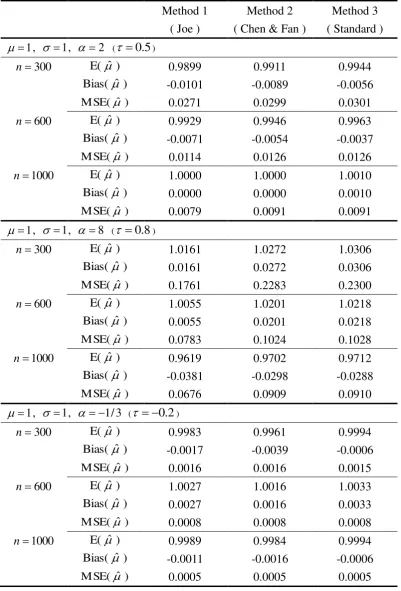
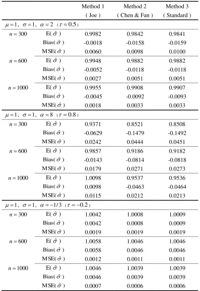
Table 1 Simulation results for ˆ based on 1000 repetitions. Method 1
( Joe )
Method 2 ( Chen & Fan )
Method 3 ( Standard )
1
, 1, 2 ( 0.5)
300
n E(ˆ ) 0.9899 0.9911 0.9944
)
ˆ
Bias( -0.0101 -0.0089 -0.0056
)
ˆ
MSE( 0.0271 0.0299 0.0301
600
n E(ˆ ) 0.9929 0.9946 0.9963
)
ˆ
Bias( -0.0071 -0.0054 -0.0037
)
ˆ
MSE( 0.0114 0.0126 0.0126
1000
n E(ˆ ) 1.0000 1.0000 1.0010
)
ˆ
Bias( 0.0000 0.0000 0.0010
)
ˆ
MSE( 0.0079 0.0091 0.0091
1
, 1, 8 ( 0.8)
300
n E(ˆ ) 1.0161 1.0272 1.0306
)
ˆ
Bias( 0.0161 0.0272 0.0306
)
ˆ
MSE( 0.1761 0.2283 0.2300
600
n E(ˆ ) 1.0055 1.0201 1.0218
)
ˆ
Bias( 0.0055 0.0201 0.0218
)
ˆ
MSE( 0.0783 0.1024 0.1028
1000
n E(ˆ ) 0.9619 0.9702 0.9712
)
ˆ
Bias( -0.0381 -0.0298 -0.0288
)
ˆ
MSE( 0.0676 0.0909 0.0910
1
, 1, 1/3 ( 0.2)
300
n E(ˆ ) 0.9983 0.9961 0.9994
)
ˆ
Bias( -0.0017 -0.0039 -0.0006
)
ˆ
MSE( 0.0016 0.0016 0.0015
600
n E(ˆ ) 1.0027 1.0016 1.0033
)
ˆ
Bias( 0.0027 0.0016 0.0033
)
ˆ
MSE( 0.0008 0.0008 0.0008
1000
n E(ˆ ) 0.9989 0.9984 0.9994
)
ˆ
Bias( -0.0011 -0.0016 -0.0006
)
ˆ
[image:28.595.79.481.116.708.2]Table 2 Simulation results for ˆ based on 1000 repetitions.
Method 1 ( Joe )
Method 2 ( Chen & Fan )
Method 3 ( Standard )
1
, 1, 2 ( 0.5)
300
n E(ˆ ) 0.9982 0.9842 0.9841
)
ˆ
Bias( -0.0018 -0.0158 -0.0159
)
ˆ
MSE( 0.0060 0.0098 0.0100
600
n E(ˆ ) 0.9948 0.9882 0.9882
)
ˆ
Bias( -0.0052 -0.0118 -0.0118
)
ˆ
MSE( 0.0027 0.0051 0.0051
1000
n E(ˆ ) 0.9955 0.9908 0.9907
)
ˆ
Bias( -0.0045 -0.0092 -0.0093
)
ˆ
MSE( 0.0018 0.0033 0.0033
1
, 1, 8 ( 0.8)
300
n E(ˆ ) 0.9371 0.8521 0.8508
)
ˆ
Bias( -0.0629 -0.1479 -0.1492
)
ˆ
MSE( 0.0242 0.0444 0.0451
600
n E(ˆ ) 0.9857 0.9186 0.9182
)
ˆ
Bias( -0.0143 -0.0814 -0.0818
)
ˆ
MSE( 0.0179 0.0271 0.0273
1000
n E(ˆ ) 1.0098 0.9537 0.9536
)
ˆ
Bias( 0.0098 -0.0463 -0.0464
)
ˆ
MSE( 0.0115 0.0212 0.0213
1
, 1, 1/3 ( 0.2)
300
n E(ˆ ) 1.0042 1.0008 1.0009
)
ˆ
Bias( 0.0042 0.0008 0.0009
)
ˆ
MSE( 0.0019 0.0019 0.0019
600
n E(ˆ ) 1.0058 1.0046 1.0046
)
ˆ
Bias( 0.0058 0.0046 0.0046
)
ˆ
MSE( 0.0012 0.0011 0.0011
1000
n E(ˆ ) 1.0046 1.0039 1.0039
)
ˆ
Bias( 0.0046 0.0039 0.0039
)
ˆ
[image:29.595.76.481.96.686.2]Table 3 Simulation results for UCL=ˆ3ˆ based on 1000 repetitions.
Method 1 ( Joe )
Method 2 ( Chen & Fan )
Method 3 ( Standard )
1
, 1, 2 ( 0.5), UCL=4
300
n E( ˆ 3ˆ) 3.9845 3.9438 3.9467
) ˆ 3 ˆ
Bias( -0.0155 -0.0562 -0.0533
) ˆ 3 ˆ
MSE( 0.0320 0.0585 0.0585
600
n E(ˆ3ˆ) 3.9773 3.9592 3.9608
) ˆ 3 ˆ
Bias( -0.0227 -0.0408 -0.0392
) ˆ 3 ˆ
MSE( 0.0152 0.0304 0.0304
1000
n E( ˆ 3ˆ) 3.9863 3.9723 3.9732
) ˆ 3 ˆ
Bias( -0.0137 -0.0277 -0.0268
) ˆ 3 ˆ
MSE( 0.0092 0.0184 0.0184
1
, 1, 8 ( 0.8), UCL=4
300
n E( ˆ 3ˆ) 3.8275 3.5834 3.5830
) ˆ 3 ˆ
Bias( -0.1725 -0.4166 -0.4170
) ˆ 3 ˆ
MSE( 0.3294 0.5220 0.5241
600
n E(ˆ3ˆ) 3.9627 3.7758 3.7765
) ˆ 3 ˆ
Bias( -0.0373 -0.2242 -0.2235
) ˆ 3 ˆ
MSE( 0.0789 0.1740 0.1738
1000
n E( ˆ 3ˆ) 3.9914 3.8314 3.8321
) ˆ 3 ˆ
Bias( -0.0086 -0.1686 -0.1679
) ˆ 3 ˆ
MSE( 0.0186 0.1083 0.1082
1
, 1, 1/3 ( 0.2), UCL=4
300
n E( ˆ 3ˆ) 4.0108 3.9987 4.0020
) ˆ 3 ˆ
Bias( 0.0108 -0.0013 0.0020
) ˆ 3 ˆ
MSE( 0.0202 0.0199 0.0200
600
n E(ˆ3ˆ) 4.0200 4.0153 4.0169
) ˆ 3 ˆ
Bias( 0.0200 0.0153 0.0169
) ˆ 3 ˆ
MSE( 0.0125 0.0121 0.0121
1000
n E( ˆ 3ˆ) 4.0126 4.0102 4.0112
) ˆ 3 ˆ
Bias( 0.0126 0.0102 0.0112
) ˆ 3 ˆ
[image:30.595.78.478.94.687.2]