Stability of Evolving Fuzzy Systems based on Data
Clouds
Hai-Jun Rong,
Member, IEEE
, Plamen Angelov,
Fellow, IEEE
,
Xiaowei Gu,
Student Member, IEEE
, and Jian-Ming Bai
Abstract—Evolving fuzzy systems (EFSs) are now well devel-oped and widely used thanks to their ability to self-adapt both their structures and parameters online. Since the concept was firstly introduced two decades ago, many different types of EFSs have been successfully implemented. However, there are only very few works considering the stability of the EFSs, and these studies were limited to certain types of membership functions with specifically pre-defined parameters, which largely increases the complexity of the learning process. At the same time, stability analysis is of paramount importance for control applications and provides the theoretical guarantees for the convergence of the learning algorithms. In this paper, we introduce the stability proof of a class of EFSs based on data clouds, which are grounded at the AnYa type fuzzy systems and the recently introduced empirical data analysis (EDA) methodological framework. By employing data clouds, the class of EFSs of AnYa type considered in this work avoids the traditional way of defining membership functions for each input variable in an explicit manner and its learning process is entirely data-driven. The stability of the considered EFS of AnYa type is proven through the Lyapunov theory, and the proof of stability shows that the average identification error converges to a small neighborhood of zero. Although, the stability proof presented in this paper is specially elaborated for the con-sidered EFS, it is also applicable to general EFSs. The proposed method is illustrated with Box-Jenkins gas furnace problem, one nonlinear system identification problem, Mackey-Glass time series prediction problem, eight real-world benchmark regression problems as well as a high frequency trading prediction problem. Compared with other EFSs, the numerical examples show that the considered EFS in this paper provides guaranteed stability as well as a better approximation accuracy.
Index Terms—Evolving Fuzzy Systems, Data Clouds, AnYa type fuzzy systems, Stability
I. INTRODUCTION
Consisting of a number of IF-THEN rules, fuzzy infer-ence systems (FISs) can deal with ill-defined and uncertain problems without precise quantitative analysis [1]. They have been applied to a wide range of areas [1]–[3]. Conventional FISs are typically built by domain experts and lack the learning capability [2], [3]. Thus, it is likely for these FISs to suffer from poor performance if inappropriate fuzzy rules are introduced. Some optimization techniques, such as back-propagation [1] or genetic algorithm [4], [5] were further
Hai-Jun Rong and Jian-Ming Bai are with State Key Laboratory for Strength and Vibration of Mechanical Structures, Shaanxi Key Laboratory of Environment and Control for Flight Vehicle, School of Aerospace, Xi’an Jiao-tong University, Shaanxi, China 710049 (e-mail:[email protected]). Plamen Angelov and Xiaowei Gu are with the School of Computing and Communications, Lancaster University, Lancaster, UK, LA1 4WA (e-mail:[email protected]). Plamen Angelov also holds an Honorary Professor title with Technical University, Sofia, Bulgaria.
applied to ensure the learning capability of the fuzzy systems. These works involve structure identification and parameter adjustment of the fuzzy systems. The structure identification of FISs aims to determine the number of fuzzy IF-THEN rules while the parameter adjustment realizes the modification of the antecedent parameters of the “IF” part and consequent parameters of the “THEN” part.
These methods, however, need to assume that all the data is available at the beginning of the training process and their training involves cycling/iterations over a number of epochs. Therefore, they are suitable for offline applications since it is hard to guarantee that these pre-trained systems have a satisfactory performance for online applications with nonsta-tionary and changeable behavior over time. To tackle this problem, in 21st century, intensive research works have been concentrated on developing evolving fuzzy systems (EFSs) [6]–[22] aiming at adapting system structure and parameters simultaneously online to capture the dynamical changes of data patterns. These include evolving rule-based models [6], dynamic evolving neuro fuzzy inference system (DENFIS) [7], a family of evolving Takagi-Sugeno (eTS) models [8]– [11], a meta-cognitive neuro-fuzzy inference system (McFIS) [12], sequential adaptive fuzzy inference system (SAFIS) [13], extended SAFIS (ESAFIS) [14], evolving possibilistic fuzzy modeling approach (ePFM) [15], multivariable Gaussian evolving fuzzy modeling system (eMG) [16], evolving fuzzy model (eFuMo) [17], incremental learning machine (PANFIS) [18], effective localist network (GENEFIS) [19], flexible fuzzy inference systems (FLEXFIS) [20], sparse fuzzy inference systems (SparseFIS) [21] and generalized smart evolving fuzzy systems (Gen-Smart-EFS) [22], etc. All these algorithms re-quire specified types of membership function to calculate the firing strength of each rule. Also, these algorithms propose different rule evolving schemes, such as density/potential criterion [6]–[11], distance criterion [16], [17], [20]–[22], error criterion [12]–[14], statistical contribution of the rule [13], [14], [18], [19]. To achieve better performance, some works further update the parameters of the membership functions using some optimization techniques, such as extended Kalman filter [12], [13]. However, these optimization techniques large-ly increase the computation complexity.
Such unmodeled dynamics are caused by linearities, non-Gaussian distributions that are much more likely to present in real problems. Some robust modification algorithms [23] are proposed to assure the stability of FISs in dealing with uncertainties. However, in these work, the fuzzy structure includes explicit membership functions which need to be fixed in advance and cannot self-evolve during training. As one of the very few examples of exiting works on stability of EFSs, an online self-organizing fuzzy modified least square (SOFMLS) network [24] was recently proposed. In this algorithm, struc-ture and parameters learning are conducted at the same time. The proposed network considers the stability analysis, but it uses unidimensional membership functions for each rule and a modified least-square algorithm to train the antecedent and consequent parameters of the system. As another example, in [25], a growing-and-pruning fuzzy neural network (GPFNN) with concurrent structure learning and parameter training is proposed, which discusses the convergence of the learning process. However, it relies on a supervised gradient decent method to update the center and width vectors of the Gaussian membership functions as well as the corresponding consequent parameters. In these works, the determination of membership function and the adjustment of antecedent parameters leads to a more complicated computation process. In both works, which are the only works on stability of EFSs we identified, explicit membership functions are considered.
Recently, a simplified type of fuzzy rule-based system was introduced, called AnYa [26], which offers a new way of defining the “IF” part of the rules without defining the membership functions per variable in an explicit manner. The antecedent parts of fuzzy rules are formed upon the data clouds, which are the sets of data samples attracted around focal points. The data clouds in the AnYa system can be formed “from scratch”. The self-evolving mechanism of the data clouds is based on determination of the focal points. In the original paper, introducing AnYa [26], focal points were identified using eClustering [27] algorithm. The importance of this approach is that AnYa type of fuzzy systems can be considered as the third alternative type of fuzzy systems to Mamdani and Takagi-Sugeno type models (both of which share same type of antecedent/IF part) with a different, explicit membership function free antecedent/IF part [27].
In this paper, we introduce a stability proof for the class of EFSs, which are based ondata clouds. The systems considered in this paper differ from the one in [26] as they form data clouds based on the empirical data analytics (EDA) [28] computational framework and empirical fuzzy sets (εFSs) [29]. EDA is a nonparametric, assumptions-free, entirely data-driven methodological framework [28] which is entirely based on the empirical observations and the ensemble properties of the data. It is close to statistical learning in its nature but is free from the assumptions required by traditional probability theory and statistical learning methods [30]. The stability of the EFS based on data clouds considered in this paper is proven through the Lyapunov theory and the proof of stability shows that the average identification error converges to a small neighborhood of zero and the parameter error is bounded by the initial parameter error. Although, the stability
proof presented in this paper specially refers to the EFSs based ondata clouds, it is applicable to some EFSs that are comprised of the structure learning of the ’IF’ part and the fuzzily weighted recursive least square parameter update of the ’THEN’ part as well.
The rest of the paper is organized as follows. The EFS based ondata cloudsis introduced in Section II. The learning process of the considered EFS including the formation of the data clouds according to EDA and the parameter learning is described in Section III. Section IV gives the stability and convergence analysis of the EFS based on data clouds. Section V presents the performance evaluation of the proposed system. This paper is concluded by Section VI.
II. EFSBASED ONDATACLOUDS
Let’s consider a nonlinear system in a discrete time frame-work expressed by:
yk=f(xk) (1)
whereyk denotes the system output,xk= [xk1,· · ·, xkn]T is the input vector of the system,f(·) is an unknown nonlinear function. Subscriptk∈ ℵis the discrete time index.
In practical cases, the exact analytical expression of the functionf(·)is hard to identify due to nonlinear and dynamic characteristics of the system. Thus, the system (1) considered in the study is unknown. To achieve the estimation of the system output yk, a fuzzy system is used to approximate the
functionf(·)as follows
ˆ
yk= ˆf(xk) (2)
whereyˆk is the output of the fuzzy system.
In this study, we consider the EFS based ondata cloudsto approximatef(·)withfˆ(·). The concept of this class of EFSs we consider is grounded at the recently introduced AnYa type fuzzy system [26].
An AnYa type fuzzy rule has the following form: Rulei: IF (xk∼γik) THEN(ˆyk isaik)
whereγi
k is the focal point of theithdata cloudin the input
space. ai
k(i = 1,2,· · ·, N)represents the crisp consequence
of theith rule that can be a constant or a linear combination of input variables. In this study, a linear consequence ai
k =
qi
k0+qii1xk1+· · ·+qiknxknis used.N represents the number
of data clouds.
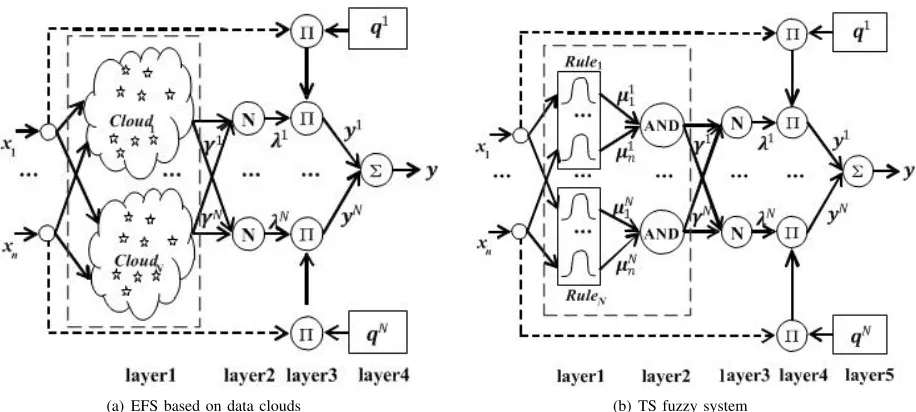
The structure of the EFS we consider is depicted in Fig. 1(a) and the structure of a traditional TS fuzzy system is given in Fig. 1(b) for comparison. One can see the difference between the two figures. The considered EFS based on data clouds consists of four layers. Layer 1 extracts the local density of eachdata cloud. The value of the local density is normalized in layer 2. Layer 3 is for applying the weighted average defuzzification. The approximated output is represented in layer 4.
(a) EFS based on data clouds (b) TS fuzzy system
Fig. 1. Structure of EFS based on data clouds (AnYa type) and traditional TS fuzzy system
approach replaces the scalar membership functions with a non-parametric function that is represented by the local densities. Considering Euclidean type of distance, in this paper, the local density of the ithdata cloud is defined as follows [28]:
γik=
1
1 + ∥xk−Γ i k∥
2
Ξi
k− ∥Γik∥2
(3)
Other types of distances can also be considered in principle, but without limiting the concept, we consider the Euclidean type of distance due to its simplicity. HereΓik andΞik are the mean and the scalar product of the data samples within the ithdata cloud. They can be updated recursively by [27]:
Γik =M i−1
Mi Γ i k−1+
1
Mixk, Γ i
1=x1
Ξik= M i−1
Mi Ξ i Mi−1+
1
Mi∥xk∥
2, Ξi
1=∥x1∥2 (4)
Mi denotes the number of data samples within the ithdata cloud.
Assuming there areN data clouds, the normalization value of the local density for each data cloudis expressed as:
λik=
γi k
∑N
i=1γki
, i= 1,2· · ·, N (5)
With the weighted average defuzzification, the output of the EFS that we consider is equal to
ˆ
yk= N
∑
i=1
λikaik;aki =xTeqik (6)
wherexe= [1,xTk]T ∈ ℜ(n+1)×1is the extended input vector
by appending the input vector xk with 1; qik is the vector
representing the consequent parameters of the kthdata cloud and given by
qik=[qik0,· · ·, qikn]T ∈ ℜ(n+1)×1 (7)
The output yˆk in Eq.(6) is further rewritten in a compact
matrix form as,
ˆ
yk=HTkQk (8)
whereQk is the consequent parameter vector of allN data
cloudsandHk is the inputs weighted by the normalized local
density vector of all data clouds. They are reformulated as,
Qk =
[
q1k,· · ·,qkN]TN(n+1)×1
Hk =
[
xT
eλ1k,· · · ,x T eλNk
]T
N(n+1)×1
(9)
Remark 1: In this EFS, the antecedent part of the fuzzy system is represented by the data clouds, and the mem-bership degree to a particular data cloud is measured by the normalized local density of the current data sample as shown in Eq. (5). This is different from the traditional fuzzy systems where the membership degree to a certain rule is determined by the normalized firing strength computed from specifically predefined membership functions based on sum-product composition. Indeed, the EFS considered in this paper does not require membership functions (also see the difference in the dashed line boxes in Figs. 1(a) and 1(b)).
III. LEARNING OFEFSBASED ON DATA CLOUDS
A. Formation of Data Clouds
In this study, the number ofdata clouds,N are determined automatically during the learning process. This enables the EFS based on data clouds to have a self-evolvable structure and to be independent from the prior knowledge about the system model. The global density defined within the EDA framework [28] is applied here as the mechanism to evolve the structure of the EFS in an online manner. Similar to the centers of fuzzy sets, each data cloud has one focal point ξ
with the highest local density. For the first data sample, it is selected as the focal point of the first data cloud, that is
cloud, its global density at thekth time instance according to EDA [28] is expressed as :
γki(G)= 1 1 + ∥Γ
i
k−ΓGk∥2 ΞG
k − ∥ΓGk∥2
(10)
whereΓGk and ΞGk are the global mean and the global scalar product of the observed data samples. The global densityγik(G) is similar to the local density, but ΓGk andΞGk consider all the samples includingxk at the current time instant,kand all the
previously observed samples xj, j= 1,2,· · ·, k−1.
When the new data sample appears, the global densities of all the existingdata cloudsare influenced and are updated ac-cordingly. The global density produced by the new observation xk according to EDA [28] is given as,
Υk=
1
1 + ∥xk−Γ G k∥
2
ΞG k − ∥Γ
G k∥2
(11)
The global density of the new data sample is compared to the updated global densities of the existing focal points to judge whether a new data cloud needs to be formed. If the global density of the new observation is higher than the global densities of the existing focal points, the new observation is more descriptive and has a stronger summarization power than all the existing focal points. In this case, the new data sample may initialize a new data cloud. On the other hand, if the new data xk is sufficiently far from the existingdata clouds,
it has a smaller global density. However, the new data sample is possible to represent a new operating regime and the new data pattern. In this case, the new data sample may be accepted as a new data cloud, even though its global density is lower than the global densities of the existing focal points. The first case is descried as follows:
(Υk−γki(G)>0) OR (Υk−γki(G)<0);∀i∈1,· · ·, N (12)
Besides the global density, the new data xk is required to
be sufficiently far from the focal points of the existing data clouds. The second case is described as:
ζki> ρik; ∀i∈1,· · ·, N (13)
whereζki denotes the distance between the current input data
xk and the focal point of the ith data clouds ξi, that is ∥xk−ξi∥.ρikrepresents the radius describing the spread of the
data cloud. It is noteworthy that the radius represents only an approximated spread of thedata cloudin the input data space because these data cloudslack a specific shape or boundary. In real implementation, the radius is hard to pre-determined and, thus, is recursively calculated based on the local ensemble information. It is updated as [11]:
ρik = 1 2(ρ
i
(k−1)+ϱ
i
k); ρi0= 1 (14)
whereϱi
krepresents the local scatter of theithdata cloudover
the input data space at thekth time instance and is expressed as,
ϱik=
√
Ξi k− ∥Γ
i
k∥2 (15)
The global density and distance information are used to evolve dynamically thedata clouds. When the condition (12) and condition (13) are both satisfied, a new data cloud is formed and the current data sample is assigned as its focal point, ξN+1 = xk. If the condition (12) and condition
(13) are not satisfied, the focal point of the nearest “data cloud” is updated by the new data, that is ξf = xk;f = argminNi=1∥xk−ξi∥. When the focal points are obtained, all
other data samples are then assigned to the nearest focal point so thatdata clouds are generated according to the following condition:
cloud label = argmini=1,2,···,N∥xk−ξi∥ (16)
After a newdata cloudis formed or an existingdata cloud is updated, xk is further utilized to update the consequent
parameters Qk of the fuzzy system (this is described in the
next subsection).
Remark 2: The system output and the evolution of thedata cloudsconsidered in this paper are based on local and global densities. But different from [26], the local and global densities used (Eq. (3) and Eq. (10)) are derived from the EDA as in [28] and inεFSs [29].
Remark 3: The EFS considered in this paper employs the global density of the new data sample and its distances to all existing focal points together as criteria to trigger the formation of new data clouds. The intrinsic self-evolving learning mechanism ensures that thesedata clouds are more general to represent all the empirically observed data samples. While condition (13) guarantees that thedata cloudsinitialised by outliers play a negligible role due to their much lower activation levels and it further avoids the overlap or conflict betweendata clouds.
B. Parameter Learning
In this subsection, the approximation mechanism of the considered EFS of the unknown nonlinear function is studied. Eq. (1) is further expressed as,
ˆ
yk=HTkQk (17)
According to the universal approximation property of fuzzy systems, there exists optimal parametersQ∗ that approximate the nonlinear dynamic functionf(·)as
yk =HTkQ∗+ϵk (18)
where ϵk is the inherent approximation error. By definition,
EFSs are capable to dynamically evolve their structure. With the number ofdata cloudsincreased, the inherent approxima-tion error can be reduced arbitrarily. Therefore, it is reasonable to assume that ϵk caused by approximating f(x)is bounded
with the constantε, which is given by
|ϵk| ≤ε (19)
On the basis of Eqs. (17) and (18), the system error becomes:
ek=yk−yˆk =HTkQ˜k+ϵk (20)
whereQ˜k = (Q∗−Qk) is the parameter error. Since, there
optimization of this EFS is simply equivalent to finding a least-square solution of the parametersQkof the consequent linear
model, which is defined as,
Jk = min k
∑
l=1
(yl−HTlQl)2 (21)
The fuzzily weighted recursive least square algorithm in-troduced in [9] is applied to update the parameters (Qk). The
adaption laws for updating the parameters Qk is defined as,
Qk+1=Qk+αkΣkHkek
Σk+1=Σk−αkΣkHkHTkΣk
(22)
whereαk is the time-varying learning rate defined as,
αk =
1 1 +HTkΣkHk
(23)
When adata cloudis added, the consequent parametersQk
becomes:
Qk= [Qk−1,qN+1]
T
(24)
with the parameters of the newdata cloud determined by:
q(N+1)i= 0, i= 0,1,2, ..., n (25)
Also, in the case that a new data cloud is added, the dimensionality of the covariance matrixΣk increases to:
Σk=
[
Σk−1 0
0 p0In+1×n+1 ]
(26)
wherep0is an initial value of the uncertainty assigned to the newly allocated rule. In the paper,p0 is set to 500 for all the cases. When the focal point of a data cloud is replaced by a new data sample, the parameters Qk and covariance matrix
Σk are inherited from the previous time step.
The pseudo-code of the EFS based on data clouds consid-ered in the paper is summarized inAlgorithm 1.
Algorithm 1Parameter Learning of EFS based on data clouds
Sample: xk ∈Rn,yk∈R Initialize: settingN = 0,ξ1=x1
1. Calculate the system output and error according to Eqs. (8) and (20).
2. Compute the global density of the existing data clouds and the new data point based on Eqs.(10)-(11).
3. Apply the rule addition criteria
if {(Υk−γki(G)>0) or (Υk−γki(G)<0)};∀i∈1,· · · , N andζki> ρik then
form a newdata cloud with
N =N+ 1,ξN+1=xk, MN+1= 1
q(N+1)i= 0, i= 0,1,2, ..., n
else
The new data sample replaces the focal point of the near-est cloud by applyingξf=xk;f = argminiN=1∥xk−ξi∥. end if
4. Adjust the consequent parameters using Eqs. (22) and (23).
IV. STABILITY ANDCONVERGENCEANALYSIS
The main contribution and novelty/originality of this paper is the theoretical proof of the stability of this class of EFSs considered here. Before describing the theorems, a useful lemma is firstly described below.
Lemma 1[31]: Define V(s) :ℜn → ℜ ≥0 as a Lyapunov
function for a nonlinear system. If there existsK∞ functions δ1(·),δ2(·), δ3(·)andK function δ4(·), and for any s∈ ℜn, each νk∈ ℜn,σ∈ ℜsatisfies
δ1(s)≤V(s)≤δ2(s)
Vk+1−Vk = ∆Vk≤ −δ3(∥νk∥) +δ4(σ)
(27)
then the nonlinear system is uniformly stable.
Theorem 1: Consider the EFS described by Eq. (8) with the self-evolving data cloud-based structure as described in sec-tion III.A. The updating equasec-tions for the parameters (Qk) are
described by Eq.(22). Then, the uniform stability of the fuzzy system described by Eq. (8) is ensured. The error between the system output and the reference output converges to a small neighborhood of zero in which the average identification error satisfies limT→∞T1∑Tk=1e2
k ≤(ε/τ)2. Here, τ is the lower
bound of αk in Eq. (23) satisfying τ = min(αk), and ε is
the upper bound of the uncertainty ϵk satisfying |ϵk| < ε.
Besides, the parameter error ∥Q˜k∥ is bounded and satisfies
the inequality condition∥Q˜k∥ ≤ ∥Q˜1∥.
Proof: Consider the following Lyapunov function
Vk = ˜QTkΣ−
1
k Q˜k (28)
According to the matrix inversion lemma ( [32], p. 258),
(A+BCBT)−1=A−1− A
−1BBTA−1
C−1+BTA−1B (29)
and by selectingA−1=Σ
k,B=Hk andC−1= 1, one can
get
Σk−+11 =Σk−1+HkHTk (30)
Combining Eqs.(28) and (29), we get
Vk+1= ˜QTk+1Σ− 1
k+1Q˜k+1
= ˜QTk+1(Σ−k1+HkHTk) ˜Qk+1
= ˜QTk+1Σ− 1
k Q˜k+1+ ( ˜QTk+1Hk)2
= ( ˜Qk−αkΣkHkek)TΣk−1( ˜Qk−αkΣkHkek)
+ ( ˜QTk+1Hk)2
=Vk−2αkQ˜TkHkek+HkTΣkHkα2ke2k+ ( ˜QTk+1Hk)2 (31)
From Eqs.(20), (22) and (23), the following relationship is obtained as,
HTkQ˜k+1+ϵk=αk(HTkQ˜k+ϵk) =αkek (32)
Substituting Eq. (32) into Eq. (31) yields,
Vk+1=Vk−2 ˜QTkHk(H T
kQ˜k+1+ϵk)
+HTkΣkHk(HTkQ˜k+1+ϵk)2+ ( ˜QTk+1Hk)
2 (33)
Considering Eq. (32), Eq. (33) becomes:
Vk+1=Vk−(HTkQ˜k+1)2−HTkΣkHk(HTkQ˜k+1+ϵk)2 −2HTkQ˜k+1ϵk
Because HT
kΣkHk(HTkQ˜k+1+ϵk)2>0, Eq. (34) can be
further transformed to:
Vk+1≤Vk−(HTkQ˜k+1)2−2HTkQ˜k+1ϵk ≤Vk+ϵ2k−(H
T
kQ˜k+1+ϵk)2
≤Vk+ϵ2k−α2ke2k
(35)
Since ϵ2
k≤ε
2, Eq. (35) is further expressed as,
∆Vk ≤ −α2ke
2
k+ε
2 (36)
For the K∞ functionsδ1(·)andδ2(·)[23]
δ1(·) =N(n+ 1)min(∥Q˜k∥2)
δ2(·) =N(n+ 1)max(∥Q˜k∥2)
(37)
the following inequality holds
N(n+ 1)min(∥Q˜k∥2)≤Vk≤N(n+ 1)max(∥Q˜k∥2) (38)
In the inequality (36), α2
ke2k is a K∞ function and ϵ2k is a
K function. It is shown that both inequalities (36) and (38) satisfy the conditions of (27). According to the Lemma 1, the uniform stability of the considered EFS is ensured. By summing up both sides of inequality (36) from1up toT, we get:
T
∑
k=1
(α2ke2k−ε2)≤V1−VT (39)
Since VT >0 is bounded, Eq. (39) is re-written as,
1
T
T
∑
k=1
α2ke2k≤ε2+ 1
TV1 (40)
AsT → ∞, we obtain
lim T→∞
1
T
T
∑
k=1
α2ke2k ≤ε2 (41)
Taking τ= min(αk), one can get
lim T→∞
1
T
T
∑
k=1
e2k ≤(ε/τ)2 (42)
Since Vk≤V1, this implies that
˜
QTkΣ−k1Q˜k≤Q˜T1Σ− 1
1 Q˜1 (43)
Combining with Eq. (30), we get:
λmin(Σ−k1)≥λmin(Σ−k−11)≥λmin(Σ−11) (44)
The inequality (44) can be further transformed into
λmin(Σ−11)∥Q˜k∥2≤λmin(Σ−k1)∥Q˜k∥2≤Q˜TkΣ−
1
k Q˜k ≤Q˜T
1Σ− 1
1 Q˜1≤λmin(Σ1−1)∥Q˜1∥2
(45)
Apparently, the following inequality holds:
∥Q˜k∥ ≤ ∥Q˜1∥ (46)
Therefore, one can conclude that ∥Q˜k∥is bounded.
Remark 4: Theorem 1 states that the average error of the system converges to a small neighborhood of zero. The approximation error is caused by the parameter errors. Ideally, when the parameters of the system converge to their optimal
values, the approximation error becomes zero. In practice, zero approximation error is hard to be achieved. Instead, the approximation error obtained is only expected to be smaller than a small nonzero value. Although, the parameters cannot converge to their optimal values, the average identification error will converge to a very small value around zero. This can be further verified through the simulation studies described in the next section.
In the EFS that we consider, the number ofdata cloudsN is determined by the learning process. To further demonstrate that the stability and convergence properties will not be affected by adding of the new data cloud, we provide and prove the following theorem.
Theorem 2: Considering the EFS described by Eq. (8), when a newdata cloud is added,Qk and Σk are updated by Eqs.
(24) and (26). The stability of the system described by Eq. (8) is still ensured.
Proof: Consider the following Lyapunov function
Vk = ˜QTkΣ−
1
k Q˜k (47)
A new data cloud (N+ 1) is added. Based on Eqs. (24) and (26), Eq. (47) becomes,
Vk+1= ˜QTk+1Σ− 1
k+1Q˜k+1
= [ ˜QT k q
T N+1 ]
[
Σk 0
0 p0In+1×n+1 ]−1
[ ˜
Qk
qN+1 ]
= ˜QTkΣ−k1Q˜k+ 1
p0
qTN+1qN+1
=Vk
(48)
From Eq. (48), it can be found that the newly added data cloud has no influence on the Lyapunov functionVk. Based
on Theorem 1, the stability of the EFS described by Eq. (8) is ensured.
Remark 5: The stability proof presented in this study is specifically applicable to the EFS considered and described in this paper. However, it is also applicable to more general EFSs satisfying Eq. (8) that are comprised of the structure learning and the fuzzily weighted recursive least square parameter update method, such as eTS [9], Simpl eTS [10], ESAFIS [14], AnYa [26] and so on.
V. NUMERICALEXAMPLES
through the training data sample by sample sequentially in an online scenario, and performance comparison is conducted in terms of the testing accuracy as well as the system complexity (the number of data clouds for the proposed system and the original AnYa, the number of rules for other algorithms).
A. Box-Jenkins gas furnace problem
Box-Jenkins gas furnace problem is a well-known bench-mark problem [12], [24]. The detailed description of this problem is given in supplementary material.
TABLE I
RESULTS OFBOX-JENKINS GAS FURNACE PROBLEM
Algorithms Testing RMSE No. of Rules AnYa (eClustering) [26] 0.0166 1
CEFNS [34] 0.0207 2
eTS [9] 0.049 5
DENFIS [7] 0.1774 18
SAFIS [13] 0.071 5
Simpl eTS [10] 0.0485 3
SOFMLS [24] 0.047 5
SONFNN [33] 0.48 4
this paper 0.0107 10
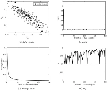
Table I compares the performance of the EFS based ondata clouds in this paper and the other algorithms. The root mean square error (RMSE) for the testing data is applied as the learning accuracy index. From the table, one can see that the considered EFS in this paper achieves the best testing accuracy compared with other algorithms. Moreover, its has a guaranteed, proven convergence, see Fig. 2(c) (and later supplementary Figs. 1(c) and 2(c)). In addition, it does not require an explicit membership function to be defined per feature/variable. For all alternative algorithms, certain type of membership functions has to be determined in advance. In SAFIS, eTS and CEFNS, Gaussian membership functions are required, while Cauchy membership function is required for the Simpl eTS. Then the parameters of membership functions are updated according to the evolving learning procedure. The focal points of the EFS described in the original AnYa paper are automatically determined through the eClustering method. Due to the different mechanisms for data clouds formation ( [26] vs [28]), the EFS in this paper achieves better testing accuracy. Fig. 2(a) shows the identified focal points and the data clouds around them. From the figure, one can see that the EFS considered in this paper generates a somewhat large number of fuzzy rules during the system identification process than other algorithms except DENFIS but achieves much better testing accuracy than all other algorithms.
Fig. 2(c) shows the evolution of the average error during the learning process. From this figure it can be observed that the average error is bounded and converges to a small neighborhood of zero, as stated in Theorem 1. Fig. 2(d) gives the evolution of the parameter αk and illustrates that the
parameter has a lower bound satisfyingαk ≥0.5. The learning
error at each time index is depicted in Fig. 2(b), from which it can be seen that the error is bounded and converges to a small neighborhood of zero.
B. Nonlinear System Identification
We further consider the nonlinear system identification problem [13], [24] as a benchmark. The problem description is given in supplementary material in details.
TABLE II
PERFORMANCE COMPARISON FOR NONLINEAR IDENTIFICATION PROBLEM
Algorithms Testing RMSE No. of Rules AnYa (eClustering) [26] 0.0546 2
CEFNS [34] 0.0183 12
DENFIS [7] 0.2599 3
ESAFIS [14] 0.0338 15
eTS [9] 0.0212 49
FlexFIS [20] 0.0171 8
SAFIS [13] 0.0221 17
Simpl eTS [10] 0.0225 22
SOFMLS [24] 0.0201 5
this paper 0.0020 9
Table II gives the testing accuracy and the number of rules obtained by different algorithms. It indicates that the EFS considered in this paper achieves much better testing accuracy with less fuzzy rules than SAFIS, ESAFIS, eTS, Simpl eTS and CEFNS, and with slightly more fuzzy rules than SOFMLS, FlexFIS and DENFIS. This table further states that the EFS considered here produces much better testing accuracy than the original AnYa. Supplementary Fig. 1(a) depicts the reference outputs and the prediction outputs of the considered EFS. The evolution of the error and the average error at each time index are presented in supplementary Fig. 1(b) and Fig. 1(c), which clearly show that they are bounded and converge to a small neighborhood of zero. The evolution of the parameter αk is
shown in supplementary Fig. 1(d) and it is clear that the error is bounded, satisfyingαk≥0.5.
C. Mackey-Glass Time Series Prediction
The fuzzy system is further evaluated by predicting the chaotic Mackey-Glass time series [13]. The detailed problem description is presented in supplementary material.
TABLE III
PERFORMANCE COMPARISON FORMACKEY-GLASS TIME SERIES PREDICTION
Algorithms Testing NDEI No. of Rules AnYa (eClustering) [26] 0.501 1
CEFNS [34] 0.303 8
DENFIS [7] 0.276 58
eTS [9] 0.356 99
FlexFIS [20] 0.157 89
ESAFIS [14] 0.312 10
SAFIS [13] 0.380 21
Simpl eTS [10] 0.376 21
this paper 0.124 17
0.75 0.8 0.85 0.9 0.95 1
y k-1
-1 -0.5 0 0.5 1
uk-4
data clouds
(a) data clouds
0 50 100 150 200
−0.2 0 0.2 0.4 0.6 0.8 1 1.2
Number of data samples
Error
(b) error
0 50 100 150 200
0 0.02 0.04 0.06 0.08 0.1
Number of data samples
Average error
(c) average error
0 50 100 150 200
Number of data samples
0 0.25 0.5 0.75 1
αk
[image:8.612.125.483.59.357.2](d)αk
Fig. 2. Evolution of focal points, averaged identification error, training error at each time index andαkfor Box-Jenkins furnace problem.
III, one can find that the EFS considered in this paper achieves a better prediction accuracy with slightly more fuzzy rules than ESAFIS, CEFNS and AnYa with eClustering, and with less rules than DENFIS, eTS, FlexFIS, SAFIS and Simpl eTS. Supplementary Fig. 2(a) and Fig. 2(b) show the evolution of the average error and error at each time index. From these figure, one can find that they are bounded. The parameterαk
is shown in supplementary Fig. 2(c) and it is clear that it is also bounded, satisfying αk ≥ 0.5. Supplementary Fig. 2(d)
depicts the reference outputs and the prediction outputs for the EFS that we consider, which indicates that they match very well.
D. Regression Problems
In this subsection, five real-world regression problems are further considered to evaluate the performance of the proposed EFS based on data clouds. Details of the problems including the attributes of input and output, the number of training and testing data are listed in supplementary Table I. In these problems, the input and output attributes are normalized in the range [0,1]. All of the training data as listed in the table is used for training and the testing data is used for verifying the generalization performance of the algorithms. Table IV presents the performance comparison between different algo-rithms. From the table, it can be found that the EFS considered here produces better testing accuracy than all other algorithms for all the problems. For the Trazines problem, DENFIS failed because of the high-dimensional input attributes and, thus, its results for this problem are not provided here. Besides, it is
obvious that in this problem the EFS considered in this paper achieves much better testing accuracy and also requires less fuzzy rules than other algorithms except CEFNS and AnYa with eClustering. This further demonstrates the advantage of the considered EFS on the high dimensional problems, in which the antecedent part of fuzzy rules is represented in a vector form and is, thus, suitable for high-dimensional problems. The curse of dimensionality problem is not going to happen for this type of EFSs thanks to the AnYa type fuzzy rules it employs.
Auto-TABLE V
STATISTICAL RESULT COMPARISON BETWEEN DIFFERENT ALGORITHMS ON THREEUCIDATA SETS.
Algorithms Auto-MPG Concrete Boston Housing
MAE±STD Max Rules/Params MAE±STD Max Rules/Params MAE±STD Max Rules/Params ANFIS [35] 2.41±0.84 4.07 16/104 11.25±9.98 39.13 8/50 3.59±1.39 6.56 4/24 AnYa (eClustering) [26] 2.50±3.17 4.57 11/88 4.84±6.45 18.16 8/64 4.38±3.77 10.26 7/98 FMCLUST [36] 2.35±0.91 3.99 20/200 7.75±2.06 12.11 3/30 2.84±1.08 5.38 6/60 FLEXFIS [20] 2.17±0.73 3.59 11/143 7.73±1.97 11.96 8/80 2.98±1.27 6.09 6/60 genfis2 [37] 2.23±0.85 3.88 6/114 8.37±1.70 11.52 3/30 3.14±1.31 6.53 4/40 Gen-Smart-EFS [22] 2.09±0.62 3.60 5.8/* 6.35±0.52 7.14 3.8/* 2.94±1.18 5.84 4.9/* SparseFIS [21] 2.01±0.55 3.29 9/144 7.73±1.77 21.01 7/70 3.02±1.19 6.04 6/60 SparseFIS uncon. [21] 2.14±0.78 4.08 22/352 8.05±1.85 12.52 11/110 3.60±1.56 6.86 19/180
this paper 1.83±0.58 2.58 13/104 4.80±1.62 16.13 11/99 2.07±1.99 3.70 14/196
TABLE IV
PERFORMANCE COMPARISON FOR REGRESSION BENCHMARK PROBLEMS
Datasets Algorithms Testing RMSE No. of Rules
Auto-MPG
AnYa (eClustering) [26] 0.0958 2
CEFNS [34] 0.0750 2
DENFIS [7] 0.1458 7
ESAFIS [14] 0.0731 33
eTS [9] 0.0864 6
McFIS [12] 0.0806 4
SAFIS [13] 0.0993 2
Simpl eTS [10] 0.0765 5
this paper 0.0725 8
Autos
AnYa (eClustering) [26] 0.0604 3
CEFNS [34] 0.0666 2
DENFIS [7] 0.4516 8
ESAFIS [14] 0.0604 3
eTS [9] 0.0535 3
McFIS [12] 0.0687 3
SAFIS [13] 0.1184 5
Simpl eTS [10] 0.0689 10
this paper 0.0399 8
AnYa (eClustering) [26] 0.0818 3
CEFNS [34] 0.0878 2
California DENFIS [7] 0.0715 14
Housing ESAFIS [14] 0.0892 6
eTS [9] 0.0772 3
McFIS [12] 0.0822 15
SAFIS [13] 0.0988 12
Simpl eTS [10] 0.0773 3
this paper 0.0711 11
AnYa (eClustering) [26] 0.0515 1
CEFNS [34] 0.0502 3
Delta DENFIS [7] 0.0497 11
Ailerons ESAFIS [14] 0.0506 13
eTS [9] 0.0513 4
McFIS [12] 0.0509 15
SAFIS [13] 0.0549 14
Simpl eTS [10] 0.0512 4
this paper 0.0491 14
Triazines
AnYa (eClustering) [26] 0.0224 6
CEFNS [34] 0.0452 6
ESAFIS [14] 0.0331 19
eTS [9] 0.0179 9
McFIS 0.0556 12
SAFIS [13] 0.0581 9
Simpl eTS [10] 0.0197 9
this paper 0.0086 7
MPG and Boston housing datasets.
E. High Frequency Trading (HFT) Prediction Problem
In this subsection, a HFT prediction problem is considered to verify the performance of the EFS based on data clouds in handling non-stationary data. The dataset is obtained from the QuantQuote Second Resolution Market Database [38] and contains tick-by-tick data on all NASDAQ, NYSE, and AMEX securities from 1998 to the present moment in time. The frequency of the tick data varies from one second to few minutes. This dataset is comprised of 19144 data samples. The inputxk includes the following five attributes: 1) Time;
2) Open price; 3) High price; 4) Low price, and 5) Close price. The task considered in the work is to predict the future 8 and 24 step values of high price, namely yk =xk+8,2 and yk =xk+24,2, respectively. The data samples are standardized online before prediction.
For comparison, two algorithms widely used in the fields of finance and economy, that is, least square linear regression (LSLR) algorithm and sliding window least square linear re-gression (SWLSLR) algorithm are considered here. Moreover, other evolving fuzzy algorithms like AnYa with eClustering, eTS, DENFIS and SAFIS are implemented for the purpose of comparison. The width of the sliding window for SWLSLR algorithm is set to 200. The NDEI and the number of rules are taken into account to evaluate the performance. Table VI shows the prediction results for 8 and 24 steps ahead. It is clear from the table that the EFS considered in this paper exhibits better prediction performance than other algorithms in both cases. Supplementary Fig. 3(a) and Fig. 3(b) show the reference and prediction outputs for the EFS based on data clouds. One can see from the two figures that the considered HFT problem here contains abnormal data samples and random fluctuations in the data stream. Large fluctuations and abnormal data frequently appear in the beginning and the end of data streams. As observed in the two figures, the EFS that we consider is capable to successfully follow the non-stationary data pattern and exhibits accurate prediction for both 8 and 24 step prediction cases with the error converging to a small value.
VI. CONCLUSIONS
TABLE VI
RESULT COMPARISON BETWEEN DIFFERENT ALGORITHMS FORHFT
PROBLEM.
Algorithms yk+8 yk+24
Testing No. of Testing No. of NDEI Rules NDEI Rules AnYa (eClustering) [26] 0.164 3 0.231 3
DENFIS [7] 1.598 12 1.582 12
eTS [9] 0.183 6 0.271 7
OLSLR [39] 0.169 / 0.242 /
SAFIS [13] 0.554 20 0.779 14
SWLSLR [40] 0.157 / 0.222 /
this paper 0.152 20 0.188 26
clouds as described in section III-A can objectively represent the local modes of the data distribution and are used as the antecedent (IF) parts of fuzzy rules. Instead of using eClustering, the method of forming data clouds described in section III-A is grounded at the empirical data analytics technique and empirical fuzzy sets, which significantly reduces the involvements of human experts and, at the same time, largely enhances the objectiveness of the fuzzy system.
The main contribution of this paper, the stability proof for the EFSs is of great importance in real applications. Nearly all the existing EFSs lack a throughout stability analysis and the very few considered the stability of the EFSs with specific types of membership functions and parameter update technique. Different from the existing works, the stability of the type of EFSs considered is proven through the Lyapunov theory and also the stability proof can be applicable to more general EFSs which satisfy Eq.(8) and are comprised of the structure learning and the fuzzily weighted recursive least square parameter update method, such as eTS [9], Simpl eTS [10], ESAFIS [14], AnYa using eClustering [26] and so on. The simulation results from the Box-Jenkins furnace problem, one system identification problem, Mackey-Glass time series prediction, 8 real-world benchmark regression problems and one high frequency trading prediction problem show that the considered EFS is not only with a theoretically guaranteed stability, but also obtains better learning accuracy. The simu-lation results also verify that the average error is bounded and converges to a small neighborhood of zero.
ACKNOWLEDGMENT
This work was supported by the National Science Council of ShaanXi Province (2014JM8337), the National Natural Science Foundation of China (61403300) and the Fundamental Research Funds for the Central Universities. This work was performed while the first author was a visiting scholar at Lancaster University.
REFERENCES
[1] J.-S. R. Jang, C.-T. Sun, and E. Mizutani,Neuro-fuzzy and soft
com-puting: a computational approach to learning and machine intelligence.
Prentice Hall, 1997.
[2] E. Mamdani, “Applications of fuzzy algorithms for simple dynamic plant,” inProceedings of IEE, vol. 121, pp. 1585–1588, 1974. [3] M. Sugeno and T. Yasukawa, “A fuzzy-logic based approach to
qual-itative modeling,” IEEE Transactions on fuzzy systems, vol. 1, no. 1, pp. 7–31, 1993.
[4] L. Wang and J. Yen, “Extracting fuzzy rules for system modeling using a hybrid of genetic algorithm and Kalman Filter,”Fuzzy Sets and Systems, vol. 101, pp. 353–362, 1999.
[5] C. W. Lee and Y. C. Shin, “Construction of fuzzy systems using least-squares method and genetic algorithm,” Fuzzy Sets and Systems, vol. 137, pp. 297–323, 2003.
[6] P. Angelov and R. Buswell, “Evolving rule-based models: A tool for
intelligent adaptation,” in Joint 9th IFSA World Congress and 20th
NAFIPS International Conference, pp. 1062–1067, 2001.
[7] N. Kasabov and Q. Song, “DENFIS: Dynamic evolving neural-fuzzy inference system and its application for time series prediction,” IEEE
Transactions on Fuzzy Systems, vol. 10, no. 2, pp. 144–154, 2002.
[8] P. Angelov and D. Filev, “On-line design of takagi-sugeno models,”
in Fuzzy Sets and Systems - IFSA 2003, International Fuzzy Systems
Association World Congress, Istanbul, Turkey, June 30 - July 2, 2003,
Proceedings, pp. 576–584, 2003.
[9] P. P. Angelov and D. P. Filev, “An approach to online identification of Takagi-Sugeno fuzzy models,”IEEE Transactions on Systems, Man, and
Cybernetics, Part B: Cybernetics, vol. 34, no. 1, pp. 484–498, 2004.
[10] P. Angelov and D. Filev, “Simpl eTS: a simplified method for learning evolving takagi-sugeno fuzzy models,” inThe 14th IEEE International
Conference on Fuzzy Systems, pp. 1068–1073, 2005.
[11] P. Angelov and X. Zhou, “Evolving fuzzy systems from data streams in real-time,” in2006 International Symposium on Evolving Fuzzy Systems, pp. 29–35, 2006.
[12] K. Subramanian and S. Suresh, “A meta-cognitive sequential learning algorithm for neuro-fuzzy inference system,”Applied Soft Computing, vol. 12, pp. 3603–3614, 2012.
[13] H.-J. Rong, N. Sundararajan, G.-B. Huang, and P. Saratchandran, “Se-quential adaptive fuzzy inference system (SAFIS) for nonlinear system identification and prediction,”Fuzzy Sets and Systems, vol. 157, no. 9, pp. 1260–1275, 2006.
[14] H.-J. Rong, N. Sundararajan, G.-B. Huang, and G.-S. Zhao, “Extended sequential adaptive fuzzy inference system for classification problems,”
Evolving Systems, vol. 2, no. 2, pp. 71–82, 2011.
[15] L. Maciel, R. Ballini, and F. Gomide, “Evolving possibilistic fuzzy mod-eling for realized volatility forecasting with jumps,”IEEE Transactions
on Fuzzy Systems, 2016.
[16] A. Lemos, W. Caminhas, and F. Gomide, “Multivariable gaussian evolving fuzzy modeling system,”IEEE Transactions on Fuzzy Systems, vol. 19, no. 1, pp. 91–104, 2011.
[17] D. Dovzan, V. Logar, and I. Skrjanc, “Implementation of an evolving fuzzy model (eFuMo) in a monitoring system for a waste water treatment process,”IEEE Transactions on Fuzzy Systems, vol. 23, no. 5, 2014. [18] M. Pratama, S. G. Anavatti, P. P. Angelov, and E. Lughofer, “PANFIS:
A novel incremental learning machine,”IEEE Transactions on Neural
Networks and Learning Systems, vol. 25, no. 1, pp. 55–68, 2014.
[19] M. Pratama, S. G. Anavatti, and E. Lughofer, “GENEFIS: Toward an effective localist network,”IEEE Transactions on Fuzzy Systems, vol. 22, no. 3, pp. 547–562, 2014.
[20] E. D. Lughofer, “FLEXFIS: A robust incremental learning approach for evolving takagisugeno fuzzy models,”IEEE Transactions on Fuzzy
Systems, vol. 16, no. 6, pp. 1393–1410, 2008.
[21] E. Lughofer and S. Kindermann, “SparseFIS: Data-driven learning of fuzzy systems with sparsity constraints,”IEEE Transactions on Fuzzy
Systems, vol. 18, no. 2, pp. 396–411, 2010.
[22] E. Lughofer, C. Cernuda, S. Kindermann, and M. Pratama, “Generalized smart evolving fuzzy systems,”Evolving Systems, vol. 6, pp. 269–292, 2015.
[23] W. Yu and X. Li, “Fuzzy identification using fuzzy neural networks with stable learning algorithms,”IEEE Transactions on Fuzzy Systems, vol. 12, no. 3, pp. 411–420, 2004.
[24] J. de Jesus Rubio, “SOFMLS: Online self-organizing fuzzy modified least-squares network,” IEEE Transactions on Fuzzy Systems, vol. 17, no. 6, pp. 1296–1309, 2009.
[25] H. Han and J. Qiao, “A self-organizing fuzzy neural network based on a growing-and-pruning algorithm,”IEEE Transactions on Fuzzy Systems, vol. 18, no. 6, pp. 1129–1143, 2010.
[26] P. Angelov and R. Yager, “A new type of simplified fuzzy rule-based system,” International Journal of Intelligent Systems, vol. 41, no. 2, pp. 163–185, 2012.
[27] P. Angelov, Autonomous Learning Systems: From Data Streams to
Knowledge in Real-time. A John Wiley&Sons, Ltd, 2012.
[28] P. Angelov, X. Gu, and D. Kangin, “Empirical data analytics,”
Interna-tional Journal of Intelligent Systems, DOI: 10.1002/int.21899, 2017.
[29] P. Angelov and X. Gu, “Empirical fuzzy sets,”to appear in International
[30] T. Hastie, R. Tibshirani, and J. Friedman, The Elements of
statisti-cal learning: Data mining, inference and prediction, Second Edition.
Springer, 2008.
[31] J. de Jesus Rubio, P. Angelov, and J. Pacheco, “Uniformly stable backpropagation algorithm to train a feedforward neural network,”IEEE
Transactions on Neural Networks, vol. 22, no. 3, pp. 356–366, 2011.
[32] N. Higham,Accuracy and Stability of Numerical Algorithms (2nd ed.). Philadelphia, PA, USA: SIAM, 2002.
[33] G. Leng, T. M. McGinnity, and G. Prasad, “An approach for on-line extraction of fuzzy rules using a self-organising fuzzy neural network,”
Fuzzy sets and systems, vol. 150, no. 2, pp. 211–243, 2005.
[34] R.-J. Bao, H.-J. Rong, P. Angelov, B. Chen, and P. K. Wong, “Correntropy-based evolving fuzzy neural system,”IEEE Transactions
on Fuzzy Systems, DOI: 10.1109/TFUZZ.2017.2719619, 2017.
[35] J.-S. Jang, “ANFIS: adaptive-network-based fuzzy inference system,”
IEEE Transactions on Systems, Man, and Cybernetics, vol. 23, no. 3,
pp. 665–685, 1993.
[36] R. Babuska,Fuzzy Modeling for Control. Boston, MA: Kluwer, 1998. [37] S. Chiu, “Fuzzy model identification based on cluster estimation,”
Journal of Intelligent and Fuzzy Systems, vol. 2, no. 3, pp. 267–278,
1994.
[38] QuantQuote Second Resolution Market Database.
https://quantquote.com/historical-stock-data.
[39] C. H. Nadungodage, Y. Xia, F. Li, J. J. Lee, and J. Ge,StreamFitter: A Real Time Linear Regression Analysis System for Continuous Data
Streams. Springer Berlin Heidelberg, 2011.
[40] K. Tschumitschew and F. Klawonn, “Effects of drift and noise on the optimal sliding window size for data stream regression models,”