Statistical Analysis on Weld Bead Geometry of Pulsed Current Micro-plasma Arc Welded AISI 316Ti Austenitic Stainless Steel Sheets

(1)

Statistical Analysis on Weld Bead Geometry of

Pulsed Current Micro-plasma Arc Welded AISI

316Ti Austenitic Stainless Steel Sheets

1

Ch. Swetha,

2

Dr. M. Murali Krishna

1,2

Department of Mechanical Engineering, Sai Ganapathi Engineering College,

Visakhapatnam, Andhra Pradesh, India

Abstract

Micro-plasma arc welding (MPAW) uses low

amperage to join sheets, where the thickness

is low, such that they can be used for

manufacturing

metal

bellows,

metal

diaphragms etc. In the present work, pulsed

current MPAW is used for joining 0.3 mm

thick AISI 316Ti austenitic stainless steel

sheets. Peak current, base current, pulse rate

and pulse width are considered as input

parameters

and

weld

bead

geometry

parameters namely front width, back width,

front height, back height are considered as

output responses. Total 27 experiments are

performed as per Box-Benhken design of

response

surface

method.

Weld

bead

geometry parameters are measured using

metallurgical

microscope.

Empirical

mathematical models are developed using

statistical software (MINITAB). Analysis of

variance (ANOVA) is carried out at 95%

confidence level. Main and interaction effects

are studied. Scatter plots are drawn to

understand the variation of actual and

predicted values of weld bead parameters.

Keywords:

Pulsed current; micro-plasma arc

welding; austenitic stainless steel; weld bead

geometry; AISI 316Ti.

INTRODUCTION

In 1964 plasma arc welding process was

introduced to the welding industry as a

method of bringing better control to the arc

welding process in lower current ranges [1]. It

is used to produce high quality welds in both

miniature and pre-precision applications and

to provide long electrode life for high

production requirements at all levels of

amperage. Plasma welding is equally suited to

manual and automatic applications. It is used

in a variety of joining operations ranging

from welding of miniature components to

seam welding, to high volume production

welding, and many others.

(2)

the anodic polarization curves in a 1 N H2SO4

solution of a 0Cr19Ni9 steel submerged arc

welded joint before and after surface melting

using a 4-A micro-plasma arc [4].

The results showed that both the heat-affected

zone and the weld metal of the as-welded joint

had a lower corrosion resistance than the as-

received parent material, while the arc melted

joint had a significantly increased corrosion

resistance. This increase in corrosion

resistance is attributed to a rapid solidification

of the melted layer. Rapid solidification of the

melted layer refines its microstructure,

decreases micro-segregation and inhibits the

precipitation of chromium carbides at the

grain

boundaries.

Karimzadeh

et

al

.

investigated the effect of micro-plasma arc

welding (MPAW) process parameters on

grain growth and porosity distribution of thin

sheet Ti6Al4V alloy weldment [5]. The

MPAW procedure was performed at different

current, welding speed and flow rates of

shielding and plasma gas. Square-butt welding

in a single pass, using direct current and

straight polarity (DCEN) was selected for the

welding process. The titanium alloy studied in

the present experiment is a thin sheet of

Ti6Al4V alloy with a thickness of 0.8 mm.

Karimzadeh

et al.

examined the effect of

epitaxial growth on microstructure of

Ti-6Al-4V alloy weldment by artificial neural

networks (ANNs) [6].

The micro-plasma arc welding (MPAW)

procedure was performed at different currents,

welding speeds and flow rates of shielding

and

plasma

gas.

Micro-structural

characterizations were studied by optical and

scanning electron microscopy (SEM). Finally,

an artificial neural network was developed to

predict grain size of fusion zone (FZ) at

different currents and welding speeds. Xu

et

al

. developed a model to simulate the

electromagnetic phenomena and fluid field in

plasma arc occurring during the low-current

micro-plasma arc welding process [7]. They

also discussed the effects of the nozzle

neck-in and weldneck-ing current of micro-plasma arc on

the arc electromagnetic field distribution.

From the works reported on plasma arc

welding, it is understood that most of the

works reported were on higher thickness; very

few works are reported on thickness less

than0.3 mm. So, it is intended to study the

effect of pulsed MPAW process parameters on

weld bead geometry parameters of 0.3 mm

thick austenitic stainless steel sheets of AISI

316 Ti, which are used for metal bellow

manufacturing. Peak current, base current,

pulse rate and pulse width are considered as

input parameters and weld bead geometry

parameters namely front width, back width,

front height, back height are considered as

output responses.

EXPERIMENTAL PROCEDURE

(3)

quality characteristics [8–11]. The values of

process parameters used in this study are the

optimal values obtained from our earlier

papers [8–11]. Hence peak current, back

current, pulse rate and pulse width are chosen

as parameters and their levels are presented in

Table 4. Details about experimental setup are

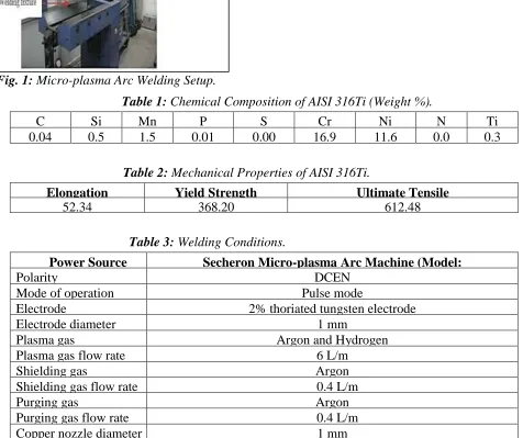
shown in Figure 1.

Fig. 1:

Micro-plasma Arc Welding Setup.

MEASUREMENT OF WELD BEAD

GEOMETRY

The weld pool geometries were measured

using inverted trinocular

metallurgical

microscope, make: BS Pyromatic, model no.:

BSPIL-MET-01013. Weld bead geometry for

sample is presented in Figure 2.

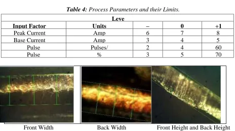
Table 1:

Chemical Composition of AISI 316Ti (Weight %).

C

Si

Mn

P

S

Cr

Ni

N

Ti

0.04

2

0.5

6

1.5

7

0.01

4

0.00

4

16.9

9

11.6

3

0.0

2

0.3

2 Table 2:

Mechanical Properties of AISI 316Ti.

Elongation

(%)

Yield Strength

(MPa)

Ultimate Tensile

Strength (Mpa)

52.34

368.20

612.48 Table 3:

Welding Conditions.

Power Source

Secheron Micro-plasma Arc Machine (Model:

PLASMAFIX 50E)

Polarity

DCEN

Mode of operation

Pulse mode

Electrode

2% thoriated tungsten electrode

Electrode diameter

1 mm

Plasma gas

Argon and Hydrogen

Plasma gas flow rate

6 L/m

Shielding gas

Argon

Shielding gas flow rate

0.4 L/m

Purging gas

Argon

Purging gas flow rate

0.4 L/m

(4)

Nozzle to plate distance

1 mm

Welding speed

260 mm/min

Torch position

Vertical

Operation type

Automatic

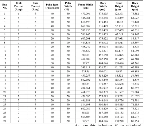
Table 4:

Process Parameters and their Limits.

Leve

ls

Input Factor

Units

–

1

0 +1

Peak Current

Amp

6

7

8 Base Current

Amp

3

4

5 Pulse

rate

Pulses/

Sec

2

0

4

0

60 Pulse

width

%

3

0

5

0

70 Front Width

Back Width

Front Height and Back Height

Fig. 2:

Weld Bead Geometry

ANALYSIS OF EXPERIMENTAL DATA

The experiments were conducted as per

the design matrix (Table 5) and the values of

weld

bead

geometry

measured

by

metallurgical microscopes are presented.

(5)

Table 5: Experimental Results.

Exp No.

Peak Current

(Amp)

Base Current

(Amp)

Pulse Rate (Pulses/sec)

Pulse Width (%)

Front Width (μm)

Back Width (μm)

Front Height (μm)

Back Height

(μm)

1 6 3 40 50 479.096 373.695 122.391 75.882

2 8 3 40 50 446.984 348.648 103.269 64.027

3 6 5 40 50 614.698 479.464 118.42 73.420

4 8 5 40 50 662.089 516.429 52.131 32.321

5 7 4 20 30 506.935 395.409 102.469 63.531

6 7 4 60 30 706.965 551.433 62.043 38.467

7 7 4 20 70 607.208 473.622 137.931 85.517

8 7 4 60 70 444.836 346.972 134.511 83.397

9 6 4 20 50 455.249 355.094 115.863 71.835

10 8 4 60 50 796.629 621.371 82.417 51.099

11 6 4 20 50 586.09 457.150 106.875 66.263

12 8 4 20 50 464.808 362.550 111.625 69.208

13 7 3 60 30 595.7 464.646 108.486 67.261

14 7 5 40 30 547.117 426.751 101.271 62.788

15 7 3 40 50 524.36 409.001 99.82 61.888

16 7 5 40 50 459.257 358.220 88.332 54.766

17 6 4 40 30 562.102 438.440 115.354 71.519

18 8 4 40 30 486.24 379.267 126.638 78.516

19 6 4 40 70 494.861 385.992 134.511 83.397

20 8 4 40 70 461.973 360.339 121.587 75.384

21 7 3 20 50 479.096 373.695 163.231 101.203

22 7 5 20 50 446.984 348.648 115.776 71.781

23 7 3 60 50 514.698 401.464 114.815 71.185

24 7 5 60 50 662.089 516.429 121.486 75.321

25 7 4 40 50 586.09 457.150 138.183 85.673

26 7 4 40 50 564.808 440.550 132.124 81.917

27 7 4 40 50 595.7 464.646 130.248 80.754

Checking the Adequacy of the

Developed Model

The adequacy of the developed model was

tested using the analysis of variance

technique (ANOVA) as shown in Table 6.

(6)

Table 6: Analysis of Variance.

Analysis of Variance for Front Width (μm)

Source DF Seq SS Adj SS Adj MS F P

Regression 14 140952 140952 10068 1.74 0.170

Linear 4 60010 13582 3396 0.59 0.678

Square 4 28396 14853 3713 0.64 0.642

Interaction 6 52546 52546 8758 1.52 0.254

Residual Error 12 69325 69325 5777

Lack-of-Fit 9 60265 60265 6696 2.22 0.277

Pure Error 3 9060 9060 3020

Total 26 210277

Analysis of Variance for Back Width (μm)

Regression 14 85755 85755 6125 1.74 0.170

Linear 4 36510 8264 2066 0.59 0.678

Square 4 17276 9037 2259 0.64 0.642

Interaction 6 31969 31969 5328 1.52 0.254

Residual Error 12 42177 42177 3515

Lack-of-Fit 9 36666 36666 4074 2.22 0.277

Pure Error 3 5512 5512 1837

Total 26 127932

Analysis of Variance for Front Height (μm)

Regression 14 8017.4 8017.37 572.67 1.10 0.438

Linear 4 4850.9 1473.02 368.25 0.71 0.602

Square 4 1363.5 1000.03 250.01 0.48 0.750

Interaction 6 1803.0 1803.03 300.50 0.58 0.742

Residual Error 12 6242.0 6242.05 520.17

Lack-of-Fit 9 6167.3 6167.26 685.25 27.49 0.010

Pure Error 3 74.8 74.79 24.93

Total 26 14259.4

Analysis of Variance for Back Height (μm)

Regression 14 3081.86 3081.86 220.133 1.10 0.438

Linear 4 1864.64 566.23 141.556 0.71 0.602

Square 4 524.12 384.42 96.104 0.48 0.750

Interaction 6 693.10 693.10 115.516 0.58 0.742

Residual Error 12 2399.41 2399.41 199.951

Lack-of-Fit 9 2370.66 2370.66 263.407 27.49 0.010

Pure Error 3 28.74 28.74 9.581

(7)

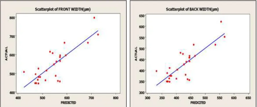
Fig. 3: Scatter Plot for Front Width. Fig. 4: Scatter Plot for Back Width.

Fig. 5: Scatter Plot for Front Width. Fig. 6: Scatter Plot for Back Height.

(8)

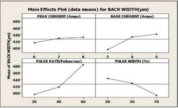
Fig. 8: Main Effect on Back Width.

Fig. 9: Main Effect on Front Height.

Surface Plots

Surface plots are drawn to identify the optimal combination of input parameters, so that desired output response is achieved. Figures 11(a) to (f) represent the surface plots for front width.

From Figure 11(a), it is understood that front width is maximum at a peak current of 6 Amps and base current of 3 Amps.

From Figure 11(b), it is understood that front width is maximum at a peak current of 6 Amps and pulse rate of 60 pulses/sec.

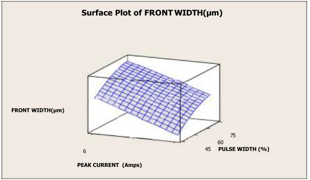
From Figure 11(c), it is understood that front width is maximum at a peak current of 6 Amps and pulse width of 70%.

From Figure 11(d), it is understood that front width is maximum at a base current of 3 Amps and pulse rate of 20 pulses/sec.

From Figure 11(e), it is understood that front width is maximum at a base current of 3 Amps and pulse width of 70%.

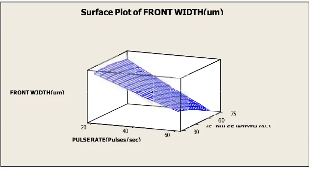
From Figure 11(f), it is understood that front width is maximum at a pulse rate of 20 pulses/sec and pulse width of 70%.

(9)

Available online:https://edupediapublications.org/journals/index.php/IJR/ P a g e | 967

Fig. 10: Main Effect for Back Height.

Fig. 11(a): Surface plot for Front Width (Peak current versus Base Current).

Fig. 11(b)

:

Surface plot for Front Width (Peak current versus Pulse Rate).

60

45 PULSE WIDTH (%)

6

Surface Plot of FRONT WIDTH(μm)

FRONT WIDTH(μm)

5

6 4 BASE CURRENT (Amps)

7 ₈ 3

PEAK CURRENT (Amps)

75

(10)

4

Fig. 11(c): Surface plot for Front Width (Peak Current versus Pulse Width).

Fig. 11(d): Surface plot for Front Width (Base Current versus Pulse Rate).

Fig. 11(e): Surface plot for Front Width (Base Current versus Pulse Width). 3

40 Surface Plot of FRONT WIDTH(μm)

60

PULSE RATE(Pulses/sec)

5 20

BASE CURRENT (Amps)

75

3

60

4

5 30

75

20 ₄₀ 45 PULSE WIDTH (%) 60

(11)

7

7 30

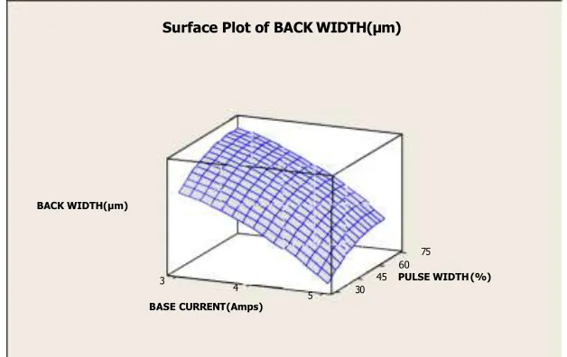
Figures 12(a) to (f) represent the surface plots for back width.

From Figure 12(a), it is understood that back width is maximum at a peak current of 6 Amps and base current of 3 Amps.

From Figure 12(b), it is understood that back width is maximum at a peak current of 6 Amps and pulse rate of 60 pulse/sec.

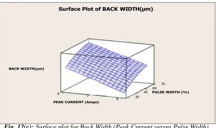
From Figure 12(c), it is understood that back width is maximum at a peak current of 6 Amps and pulse width of 70%.

From Figure 12(d), it is understood that back

width is maximum at a base current of 3 Amps and pulse rate of 60 pulse/sec.

From Figure 12(e), it is understood that back width is maximum at a base current of 3 Amps and pulse width of 70%.

From Figure 12(f), it is understood that back width is maximum at a pulse rate of 20 pulses/sec and pulse width of 60%.

From all the surface plots, it is understood that back width is maximum when peak current is 6 Amps, base current is 3 Amps, pulse rate of 60 pulses/sec and pulse width of 70%.

Fig. 12(a): Surface plot for Back Width (Peak current versus Base Current).

Fig. 12(b): Surface plot for Back Width (Peak current versus Pulse Rate).

Fig. 12(c): Surface plot for Back Width (Peak Current versus Pulse Width). 60

6

40 6

Surface Plot of BACK WIDTH(μm)

BACK WIDTH(μm)

60

BACK WIDTH(μm)

75

8 20

8

(12)

4

4 30

40 30

Fig. 12(d): Surface plot for Back Width (Base Current versus Pulse Rate).

Fig. 12(e): Surface plot for Back Width (Base Current versus Pulse Width).

Fig. 12(f): Surface plot for Back Width (Pulse Rate versus Pulse Width). 60

20

60

3

40 3

Surface Plot of BACK WIDTH(μm) vs PULSE

BACK WIDTH(μm)

60

BACK WIDTH(μm)

75

BACK WIDTH(μm)

75

5 20

5

(13)

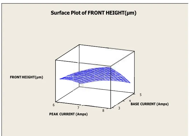
Figures 13(a) to (f) represent the surface plots for front height.

From Figure 13(a), it is understood that front height is minimum at a peak current of 6 Amps and base current of 5 Amps.

From Figure 13(b), it is understood that front height is minimum at a peak current of 6 Amps and pulse rate of 60 pulses/sec.

From Figure 13(c), it is understood that front height is minimum at a peak current of 6 Amps and pulse width of 70%.

From Figure 13(d), it is understood that front

height is maximum at a base current of 3 Amps and pulse rate of 60 pulses/sec.

From Figure 13(e), it is understood that front height is minimum at a base current of 3 Amps and pulse width of 60%.

From Figure 13(f), it is understood that front height is minimum at a pulse rate of 20 pulses/sec and pulse width of 60%.

From all the surface plots, it is understood that front height is minimum when peak current is 6 Amps, base current is 3 Amps, pulse rate of 60 pulses/sec and pulse width of 70%

Fig. 13(a): Surface plot for Front Height (Peak current versus Base Current).

Fig. 13(b): Surface plot for Front Height (Peak current versus Pulse Rate).

Surface Plot of FRONT HEIGHT(μm)

FRONT HEIGHT(μm)

5

7 ₈ 3

200

100

60

0 ₄₀

6 PULSE RATE(Pulses/sec)

7

8 20

(14)

Fig. 13(c): Surface plot for Front Height (Peak Current versus Pulse Width).

Fig. 13(d): Surface plot for Front Height (Base Current versus Pulse Rate).

Fig. 13(e): Surface plot for Front Height (Base Current versus Pulse Width). Surface Plot of FRONT HEIGHT(μm)

75

6

60

7

8 30

RONT HEIGHT(μm)

60 40

4

5 20

75

3

60

4 ₅ 30

(15)

Fig. 13(f): Surface plot for Front Height (Pulse Rate versus Pulse Width).

Figures 14(a) to (f) represent the surface plots for back height.

From Figure 14(a), it is understood that back height is minimum at a peak current of 6 Amps and base current of 5 Amps.

From Figure 14(b), it is understood that back height is minimum at a peak current of 6 Amps and pulse rate of 60 pulses/sec.

From Figure 14(c), it is understood that back height is minimum at a peak current of 6 Amps and pulse width of 75%.

From Figure 14(d), it is understood that back

height is maximum at a base current of 3 Amps and pulse rate of 60 pulses/sec.

From Figure 14(e), it is understood that back height is minimum at a base current of 3 Amps and pulse width of 60%.

From Figure 14(f), it is understood that back height is minimum at a pulse rate of 20 pulses/sec and pulse width of 70%.

From all the surface plots, it is understood that back height is minimum when peak current is 6 Amps, base current is 3 Amps, pulse rate of 60 pulses/sec and pulse width of 70%

Fig. 14(a): Surface plot for Back Height (Peak current versus Base Current).

Surface Plot of BACK HEIGHT(μm)

BACK HEIGHT(μm)

5

7 3

8 PEAK CURRENT (Amps)

75

20

60

40 ₆₀ 30

(16)

Fig. 14(b): Surface plot for Back Height (Peak current versus Pulse Rate).

Fig. 14(c): Surface plot for Back Height (Peak Current versus Pulse Width).

Fig. 14(d): Surface plot for Back Height (Base Current versus Pulse Rate).

60 40

7

8 20

75

6

60

7

8 30

60 40

4 ₅ 20

(17)

Fig. 14(e): Surface plot for Back Height (Base Current versus Pulse Width)

Fig. 14(f): Surface plot for Back Height (Pulse Rate versus Pulse Width).

CONCLUSIONS

From the experiments and developed models the following conclusions are drawn:

 Empirical mathematical models are

developed for front width, back width, front height and back height of weld bead

in order to predict their values within the range of the welding parameters selected for the chosen material (AISI 316Ti).

 The adequacy of the developed model is checked using ANOVA at 95% confidence level and found to be adequate.

 From the scatter plot it is understood that

Surface Plot of BACK HEIGHT(μm)

BACK HEIGHT(μm)

75

3

60

45 PULSE WIDTH (%)

4

5 30

BASE CURRENT (Amps)

75

20

60

40 ₆₀ 30

(18)

experimental and predicted values are close to each other.

 Front width and back width increase with increase in peak current, back current and pulse rate. However they decrease with increase in pulse width.

 Front height and back height decrease with increase in peak current, back current and pulse rate. However they increase with increase in pulse width.

 From the surface plots of front width and back width, it is understood that maximum front width and back width can be achieved when peak current is 6 Amps, base current 3 Amps, pulse rate of 60 pulses/sec and pulse width of 70%.

 From the surface plots of front height and back height, it is understood that front height is minimum when peak current is 6 Amps, base current is 3 Amps, pulse rate of 60 pulses/sec and pulse width of 70%.

 From all the surface plots, it is understood that optimal weld bead geometry is obtained when peak current is 6 Amps, base current is 3 Amps, pulse rate of 60 pulses/sec and pulse width of 70%

 The developed mathematical models for weld bead geometry parameters are valid only for 0.3 mm thick AISI 316Ti austenitic stainless steel.

 The developed model is valid within the specified range of the selected welding parameters; however the accuracy can be improved by considering more number of factors and their levels.

REFERENCES

[1] Jean Marie Fortain. Plasma Welding

Evolution & Challenges. Air Liquid CTAS,

Welding and Cutting Research Center, 95315, Cergy Pontoise, France. 2010; 11p. [2] Voropai NM, Shcherbak VV, Grigorev

AA. Pulsed Microplasma Welding of Thin

Aluminum Gaskets. Equipment

Manufacturing Technology. 1971; 11: 19p. [3] Sepokurov AS, Sergatskii GI, Alikin

AP. Use of Microplasma Welding in

Component Construction. Japan Welding Society. 1971; 11: 20p.

[4] Luo W. Effect of Micro-Plasma Arc Melting on the Corrosion Resistance of a 0Cr19Ni9 Stainless Steel SAW Joint. Mater Lett. 2002; 55: 290–295p.

[5] Karimzadeh F, Salehi M, Saatchi A, et al. Effect of Microplasma Arc Welding Process Parameters on Grain Growth and Porosity Distribution of Thin Sheet Ti6Al4V Alloy Weldment. Mater Manuf Processes. 2005; 20(2): 205–219p.

[6] Karimzadeh F, Ebnonnasir A, Foroughi A. Artificial Neural Network Modeling for Evaluating of Epitaxial Growth of Ti6Al4V Weldment. Mater Sci Eng. 2006; A 432: 184–190p.

[7]Pei-quan Xu, Shun Yao, Jian-Ping He, et al. Numerical Analysis for Effect of Process Parameters of Low-Current Micro-PAW on Constricted Arc. Int J Adv Manuf Technol. 2009; 44: 255–264p.

[8]Kondapalli Siva Prasad, Ch. Srinivasa Rao, Nageswara Rao D. Application of Grey Relational Analysis for Optimizing Weld Pool Geometry Parameters of Pulsed Current Micro Plasma Arc Welded Inconel 625 Sheets. Int J Adv Manuf Technol, (Springer). 2015. DOI: 10.1007/s00170-014-6665-y.

[9]Siva Prasad K, Ch. Srinivasa Rao, Nageswara Rao D. Effect of Process Parameters of Pulsed Current Micro Plasma Arc Welding on Weld Pool Geometry of Inconel 625 Welds. Kovove

Materialy-Metallic Materials (Kovove

Mater). 2012; 0(3): 153–159p.