warwick.ac.uk/lib-publications
Manuscript version: Author’s Accepted Manuscript
The version presented in WRAP is the author’s accepted manuscript and may differ from the published version or Version of Record.
Persistent WRAP URL:
http://wrap.warwick.ac.uk/114595
How to cite:
Please refer to published version for the most recent bibliographic citation information. If a published version is known of, the repository item page linked to above, will contain details on accessing it.
Copyright and reuse:
The Warwick Research Archive Portal (WRAP) makes this work by researchers of the University of Warwick available open access under the following conditions.
Copyright © and all moral rights to the version of the paper presented here belong to the individual author(s) and/or other copyright owners. To the extent reasonable and
practicable the material made available in WRAP has been checked for eligibility before being made available.
Copies of full items can be used for personal research or study, educational, or not-for-profit purposes without prior permission or charge. Provided that the authors, title and full
bibliographic details are credited, a hyperlink and/or URL is given for the original metadata page and the content is not changed in any way.
Publisher’s statement:
Please refer to the repository item page, publisher’s statement section, for further information.
A statistical test on the local effects of spatially structured variance
Spatial variance is an important characteristic of spatial random variables. It describes local deviations from average global conditions and is thus a proxy for spatial heterogeneity. Investigating instability in spatial variance is a useful way of detecting spatial boundaries, analysing the internal structure of spatial clusters and revealing simultaneously acting geographic phenomena. Recently, a corresponding test statistic called ‘Local Spatial Heteroscedasticity’ (LOSH) has been proposed. This test allows locally heterogeneous regions to be mapped and investigated by comparing them with the global average mean deviation in a dataset. While this test is usefulin stationary conditions, its value is limited in a global heterogeneous state. There is a risk that local structures might be overlooked and wrong inferences drawn. In this article, we introduce a test that takes account of global spatial heterogeneity in assessing local spatial effects. The proposed measure, which we call ‘Local Spatial Dispersion’ (LSD), adapts LOSH to local conditions by omitting global information beyond the range of the local neighbourhood and by keeping the related inferential procedure at a local level. Thereby, the local neighbourhoods might be small and cause small-sample issues. In the view of this, we recommend an empirical Bayesian technique to increase the data that is available for resampling by employing empirical prior knowledge. The usefulness of this approach is demonstrated by applying it to a LiDAR-derived dataset with height differences and by making a comparison with LOSH. Our results show that LSD is uncorrelated with non-spatial variance as well as local spatial autocorrelation. It thus discloses patterns that would be missed by LOSH or indicators of spatial autocorrelation. Furthermore, the empirical outcomes suggest that interpreting LOSH and LSD together, is of greater value than interpreting each of the measures individually. In the given example, local interactions can be statistically detected between variance and spatial patterns in the presence of global structuring, and thus reveal details that might otherwise be overlooked.
Keywords: spatial analysis; spatial heterogeneity; spatial hypothesis testing; spatial non-stationarity
1. Introduction
Despite its useful properties, spatial heterogeneity plays a relatively minor role in spatial analysis techniques, which are mostly designed for clustering. Measures of spatial autocorrelation and hot spot techniques are prevalent, and these are used to assess associations within spatial random variables (Getis 2010). In contrast, spatial heterogeneity is often deemed to be a technical nuisance and seldom regarded as a source of valuable information. It either requires a methodological approach (Anselin 1988, Páez and Scott 2004, Graif and Sampson 2009), or is considered to be reminiscent of large-scale structures that influence local patterns (e.g., Ord and Getis 2001). Spatial heterogeneity indeed undermines the stationarity assumptions that form the basis of many spatial techniques (Gaetan and Guyon 2010, p. 166 ff.). Thus, regarding it from the standpoint of a nuisance is partly justified.
Nonetheless, spatial heterogeneity often contains useful information. A good illustration of this is the recent investigation of the domiciles of newly arrived migrants from rural areas to Accra, Ghana (Getis 2015). The use of spatial variance as a proxy for spatial heterogeneity allows transitional zones to be detected between the underdeveloped and wealthy districts of the city. Incoming migrants from rural parts of Ghana first settle in these transitional areas after they first arrive in the city. This recent example shows that spatial heterogeneity can supply important information to investigations of complex geographic situations, and lead to useful conclusions of both a theoretical and practical value.
Spatial heterogeneity is also important for the analysis of intrinsically heterogeneous and novel data sources. Social media data, for instance, are sometimes called the ‘big noise’ (Lovelace et al. 2016), because they are characterised by unstable ‘wild variance’ (Jiang 2015). The latter is characterised by an interaction between spatial patterns and variance, which influences analysis results. Westerholt et al. (2015, 2016) recently found that spatial heterogeneity causes Type I errors, topological outliers and some further problems that are relevant to the spatial analysis of Twitter data. As a result, many researchers are now investigating social media data in an attempt to mitigate its noisy features (e.g., Sengstock et al. 2013, Lovelace et al. 2016, Steiger et al. 2016). The investigation of heterogeneity, however, might provide a clue about the spatial perceptions of people and help to characterise the users’ everyday behaviours more accurately. Similar arguments hold true for the data obtained from multi-temporal analysis. The differences between multi-temporal data acquired by ‘Light Detection and Ranging’ (LiDAR) (Fang and Huang 2004, Tian et al. 2014), for example, are a means of detecting heterogeneous changes in surface phenomena. When investigating the LiDAR recordings of landslides (Jaboyedoff et al. 2012), it was found that spatial heterogeneity can provide a wealth of information about significant morphological features like differently shaped earth deposits (Hungr et al. 2014). These two rather different examples demonstrate the potential value of investigating spatial heterogeneity in a number of application scenarios.
from the global average variability. The measure thus reveals and maps structures of the variance that are at least partially global in nature, whereas the weaker structures that are entirely local remain hidden. The latter only feature prominently in local circumstances but remain undetected by the global reference framework of LOSH.
We set out a technique that extends LOSH by making it a measure for the influence of local spatial patterns on local variance. The test, which we call ‘Local Spatial Dispersion’ (LSD), makes it possible to detect whether the local geographic arrangement of random variables increases or reduces the variance. This is carried out in an entirely local manner and takes no account of global characteristics. In addition, we propose an entirely local bootstrapping approach for drawing inferences. Drawing inferences that are only local, however, entails limited amounts of data from small local neighbourhoods. As a means of circumventing the problem of small-size samples within these local subsets, (which particularly arises when adjusting small analytical scales), the inference technique includes an empirical Bayesian prediction of additional synthetic local data. The usefulness of the proposed technique can be demonstrated by applying it to a high-resolution 3D change detection dataset. The data is derived from a long-term ‘automatic terrestrial laser scanning station’ (ATLS) that covers a slow-moving landslide in Gresten, Austria and provides a useful scenario because it contains both a distinct global structure and additional local patterns.
The paper starts with a detailed review of spatial heterogeneity and spatial heteroscedasticity, and includes a brief discussion of related statistical methodologies (Section 2). Following this outline, LOSH and our proposed measure are introduced (Sections 3 and 4). Then, there is a Bayesian prediction of residuals as well as the bootstrap method for developing predictive models (Section 5), before the empirical results are discussed (Session 6) and the final conclusions are drawn (Section 7).
2. Related work: Spatial heterogeneity and spatial heteroscedasticity
Different structural types of spatial heterogeneity are distinguishable. These are characterised by their causal origins, maintenance mechanisms, spatial structures, and functional and temporal dynamics (Strayer et al. 2003). Other more technical distinguishing factors include the types of investigated variables (Wagner and Fortin 2005), the underlying spatial indexes (spatially discrete vs. continuous; Anselin 2010) and even the methodological perspectives that researchers adopt (dynamic modelling vs. hypothesis testing; Fagan et al. 2003). In structural terms, heterogeneous zones sometimes condense to thin and crisp boundaries, while they can also appear fuzzy (Jacquez et al. 2000).
For functional purposes, heterogeneous zones can act as semipermeable filters or conduits and as devices from which spatial processes either originate or where they are impeded (Forman 1995). Steep gradients or threshold conditions, at which variable states change suddenly, can also be found in heterogeneous areas (Fagan et al. 2003). These characteristics allow the spatial heterogeneity to exert a short or long-range influence on dynamic processes (Fagan et al. 2003). Sometimes these influences get strengthened by the interrelations between the effects mentioned earlier, especially by the interplay between the structural and functional characteristics (Laurance et al. 2001). Hence, the various features, together with the number of functional influences, show the importance of investigating spatially heterogeneous zones.
Techniques to detect heterogeneous zones (especially crisp boundaries), first appeared in image processing. Some corresponding methods have been designed for segmenting synthetic images, although they are not capable of depicting dynamic real-world systems in their entirety (Goovaerts 2010). A range of more suitable methods has thus evolved, including techniques based on moving split-windows (Fortin 1994, 1999, Kent et al. 1997, 2006), first-order derivatives (‘Wombling’, Womble 1951, Barbujani et al. 1989, Gelfand and Banerjee 2015), second-order derivatives (Fagan et al. 2003, Lillesand et al. 2015), spatially constrained clustering (Jacquez et al. 2000, Patil et al. 2006, Bravo and Weber 2011), fuzzy set modelling (Arnot and Fisher 2007, Fisher and Robinson 2014), wavelets (Csillag and Sándor 2002, Keitt and Urban 2005, Ye et al. 2015) and several further parametric as well as non-parametric techniques (Jacquez et al. 2008, Wang et al. 2016). Another closely related research field is concerned with integrating spatial heterogeneity with quantitative models. The respective approaches include the following: hierarchical and Bayesian concepts (Lee and Mitchell 2012, Anderson et al. 2014, Hanson et al. 2015), geostatistical techniques (Garrigues et al. 2006, Goovaerts 2008, Hu et al. 2015), extensions to global spatial regression methods (Anselin 2001), and the local geographically-weighted regression approach (Fotheringham et al. 1996, 2002, Brunsdon et al. 1998).
in different parameters and also between the three parts outlined above, to achieve a thorough understanding of the behaviour of random variables and related phenomena.
In spatial analysis, varying means are analysed by hot spot techniques like the G and the O-statistic (Getis and Ord 1992, Ord and Getis 1995, 2001). By analogy, variations caused by autocorrelation are analysed through local measures of spatial autocorrelation like the ‘Local Indicators of Spatial Association’ (LISA, Anselin 1995). While these cases have been widely investigated, there has been comparatively little research on variability in the variance (called ‘spatial heteroscedasticity’; Dutilleul and Legendre 1993). Roughly speaking, spatial heteroscedasticity refers to ‘wild variance’ (Jiang 2015). Ord and Getis (2012) recently put forward a local measure called ‘Local Spatial Heteroscedasticity’ (LOSH), which assesses spatial structure in variance and is akin to a spatial χ² test. Xu et al. (2014) investigated the distributional properties of LOSH and found that the χ² approximation proposed by Ord and Getis (2012) is not always suitable, and that a Monte Carlo bootstrap should be used instead.
LOSH is ideally suited to detecting boundary-like sub-regions lying between homogeneous regimes. However, it cannot describe in detail how local spatial arrangements of random variables in place affect the heterogeneity within the individual sub-regions. This is where our study is able to make a contribution to the field because it supplements LOSH by conducting a test involving the local spatial microstructure of the variance of georeferenced random variables.
3. Local spatial heteroscedasticity (LOSH)
The LOSH measure (Ord and Getis 2012) calculates local deviations from the global average variance. It is derived from the hot spot technique called ‘G-statistic’ (Getis and Ord 1992, Ord and Getis 1995) and allows boundaries and hot spots of high variability to be detected. LOSH tests the following hypotheses:
𝑯𝟎𝑳𝑶𝑺𝑯: The variance in a region does not deviate markedly from its global average.
𝑯𝟏𝑳𝑶𝑺𝑯: The variance in a region deviates from overall variance homogeneity.
entire geographic layout to those geographic features that are relevant to a particular phenomenon under study. These weights can be of an arbitrary shape (s. Bavaud 2014 for an overview) and no specific form is required for the remainder. LOSH (Hi is the notation for LOSH chosen by (Ord and Getis 2012)) then reads as
𝐻𝑖 = ∑ 𝑤𝑖𝑗|𝑒𝑗|
𝑎 𝑗∈𝒩
ℎ1∑𝑗∈𝒩𝑤𝑖𝑗 , 𝑒𝑗 = 𝑥𝑗− 𝑥̅𝑗, 𝑥̅𝑗 =
∑𝑘∈𝒩𝑗𝑤𝑗𝑘𝑥𝑘
∑𝑘∈𝒩𝑗𝑤𝑗𝑘 and ℎ1 =
∑ |𝑒𝑗| 𝑎 𝑗∈𝒩
𝑛 , (1)
where ej is a residual about a local spatially weighted mean x̅j and h1 is the overall average residual estimated from all the spatial units in the region. Note that 𝒩j is the neighbourhood around unit j, that is defined analogously to 𝒩i. Exponent a allows different types of mean deviations to be investigated. For the remainder of this paper, we adjust a = 2 and confine the discussion to a measure of variance.
An inference about LOSH assumes random permutations of the residuals. When an average residual h1 is employed, it thus makes clear that LOSH assumes weak stationarity in the null hypothesis. The successful detection of a local pattern thus depends on the global reasonability of h1. Through a random permutation of the residuals, the statistic obtains an expected value of 𝐸[𝐻𝑖] = 1 and has a variance of
𝑉𝑖[𝐻𝑖] = 1 𝑛−1(
1 ℎ1∑𝑗∈𝒩𝑤𝑖𝑗)
2
[1
𝑛(∑ |𝑒𝑗| 2𝑎
𝑗∈𝒩 − [∑ |𝑒𝑗|
𝑎
𝑗∈𝒩 ]
2
)] (𝑛 ∑𝑗∈𝒩𝑤𝑖𝑗2− [∑𝑗∈𝒩𝑤𝑖𝑗] 2
). (2)
Ord and Getis (2012) propose an adjusted χ² approximation to the null distribution as a parametric solution to statistical inference. The χ² distribution stems from the design of the statistic as a spatialised variant of the classic χ² test for testing deviations from a hypothesised variance. This is seen by writing out the individual terms of the sum from Equation (1):
𝐻𝑖 = 𝑤𝑖1
∑𝑗∈𝒩𝑤𝑖𝑗
|𝑒1|2
ℎ1 + ⋯ +
𝑤𝑖𝑗
∑𝑗∈𝒩𝑤𝑖𝑗
|𝑒𝑗| 2
ℎ1 + ⋯ +
𝑤𝑖𝑛
∑𝑗∈𝒩𝑤𝑖𝑗
|𝑒𝑛|2
ℎ1 . (3)
Variable h1 is the hypothesised variance and the summands are (spatially weighted) squared standardised residuals. Under normality constraints, these are χ² with one degree of freedom. Their sum is then χ² with additive degrees of freedom (Cochran 1934). On the basis of the findings from Box (1953), Ord and Getis (2012) adjust LOSH to take better account of non-normality by including the empirical variance Vi. This matches the χ² approximation to the observed outcomes and controls the shape of the reference distribution. The skew and the excess kurtosis of the reference distribution are given by 𝛾1 = 2√𝑉𝑖 and 𝛾2 = 6𝑉𝑖, and the test statistic is 𝑍𝑖 = 2𝐻𝑖/𝑉𝑖 with 2/𝑉𝑖
4. Local spatial dispersion (LSD)
Instead of comparing local regions with a global average like LOSH, the proposed measure LSD is concerned with the effect of the local spatial pattern on local variances. The underlying assumption is that the way random variables are arranged geographically increases or reduces the variance, or else is unrelated to its characterisation. The measure is only defined in a local context and does not take account of global information. The same principle also applies for the related inference procedure, which is conducted locally.
The proposed LSD is useful when a dataset comprises statistically differing sub-regions or when spatially coexisting phenomena are observed. However, global information such as the average residual h1 is not meaningful in these circumstances. This means the LOSH approach causes problems because it is unrealistic to assume there is weak stationarity in these cases. Instead, the variance patterns might be strongly interacting with the geographic layout locally, although they might not be recognised when a global comparison is made with sub-regions that show a stronger dispersal. Thus LOSH cannot be employed to assess entirely local effects and an entirely local measure of spatial variance, such as LSD, can prove to be useful.
4.1 Hypotheses
The proposed test determines whether the local spatial arrangement of random variables increases or reduces the local variance. The following two hypotheses for LSD are formulated:
𝑯𝟎𝑳𝑺𝑫:The local geographic layout has no systematic effect on the variance. 𝑯𝟏𝑳𝑺𝑫:The local geographic layout causes local over- or underdispersion.
The null model assumes that the local variance is unrelated to the geographic arrangement. If the null is accepted, it means that the investigated data gives no indication that geographical factors are responsible for the variance effects. Note that variability can still be related to its particular location. The average level of variability is still treated as a function of location. This is achieved through a local average residual hi (see Equation 5). However, LSD tests the local spatial influence on the dispersal behaviour above the general local variability level. In conceptual terms, the hypothesis testing scheme of 𝐻0𝐿𝑆𝐷 and 𝐻1𝐿𝑆𝐷 derives from a linear autoregressive framework. Let
Ε𝑖 = (|𝑒𝑗| 𝑎
)
𝑗 with j ∈ 𝒩i be a vector of exponentiated residuals from a local
neighbourhood i with ej as defined in Equation (1). Let 𝛼𝑖 = 𝐸[|𝑒𝑗|𝑎] be the expected (non-geographic) exponentiated residual within a local neighbourhood i. The two presented hypotheses can be derived from a linear regression model:
𝔢𝑖 = 𝛼𝑖 + 𝜌𝑖𝑊𝑖𝑇Ε𝑖 + 𝜀𝑖, (4)
model occurs when the coefficient ρi is close to zero. Hence, LSD tests to what degree this coefficient deviates from zero. If a left-side test is conducted, the alternative model represents a significantly negative ρi. Its acceptance thus means that the geographic arrangement, as defined through W, reduces the variance more than it would be the case when geographical factors have no effect. By analogy, acceptance of the alternative in a test on the right-side indicates a significantly positive magnitude of ρi, which means that the local geography increases the variability within the random variables. The hypotheses outlined here are thus useful devices to test the role of geographic layout in the local dispersal behaviour of the spatial random variables.
4.2 Mathematical definition
The LSD measure is formulated mathematically as a ratio of the spatially weighted local residuals and their own spatially randomised local average. Therefore, LSD is given by
𝐿𝑆𝐷𝑖 = ∑ 𝑤𝑖𝑗|𝑒𝑗|
𝑎 𝑗∈𝒩
ℎ𝑖∑𝑗∈𝒩𝑤𝑖𝑗 , ℎ𝑖 =
∑ |𝑒𝑗|
𝑎 𝑗∈𝒩𝑖
𝑛𝑖 , (5)
where ni denotes the cardinality of 𝒩i and hi is the local mean residual. Residuals ej are as defined in Equation 1. The term hi is a replacement of h1 and allows a strictly local analysis to be conducted. The datasets can thus be heterogeneous with regard to mean and variance. This important difference from LOSH is further illustrated through the relationship between LOSH and LSD (Appendix A):
𝐿𝑆𝐷𝑖 =𝐻𝑖⋅ℎ1
ℎ𝑖 . (6)
Equation (6) shows that LSD is a rescaled version of LOSH. Whenever hi equals h1, LOSH and LSD are equivalent. This is the case when the local variability equals the global average dispersal behaviour. LSD is particularly valuable when hi < h1, because LOSH tends to overlook these kinds of weak local structures. In contrast, LSD adapts to specific local conditions and enables truly local variance patterns to be investigated. On the contrary, local deviations detected by LOSH are, at least in part, caused by global instability in the first two moments.
5. Inference procedure
Two issues complicate the task of making inferences about LSD: potential deviations from normality and the constraint of having to keep the inference local. In the case of normal attributes, LSD can technically be evaluated as a χ² test, even though the mean and variance might vary (Walck 2007, p. 38). However, in the light of the results of Xu et al. (2014), we do not want to restrict the test to normal populations that seldom occur in real geographic conditions. Furthermore, the intended local nature of an inference approach might cause problems by the small-size local samples. This is particularly the case when the analytical scale is small. In such cases, there is a serious lack of data available for local resampling and bootstrap distributions are unreliable. The χ² approach is thus not applicable and a different inferential strategy is required.
A two-step approach is put forward as a means of overcoming this difficulty: (1) A Bayesian prediction of synthetic data to increase the size of the local database
through
(a) determining suitable prior distributions and
(b) a Bayesian updating for adjusting priors to local conditions. (2) Arranging of local bootstrap distributions using the data from step 1.
The Bayesian approach in the first stage is used to boosting the amount of available data. The purpose of this is to predict additional local mean values, from which auxiliary residuals can be generated. These can then be plugged into LSD during the Monte Carlo iterations in the bootstrap. The second stage describes the final estimation of a reference distribution that is used for inference purposes. The following sub-sections outline these two stages in more detail.
5.1 Bayesian mean prediction
The first part in the inferential approach is to supply the available local subsets with additional information. This is carried out by predicting the synthetic mean values that are used for drawing additional local residuals. The mean estimation is subject to the central limit theorem. This allows us to exploit the advantage of well-known a priori knowledge about the underlying distributional characteristics of mean estimations. Arithmetic means converge to normal distributions. Predicting the means is thus conceptually simpler than drawing the residuals, and for this reason, we have chosen to follow this path rather than predicting residuals directly.
outlined two-step approach reduces the risk of adapting to local situations too far by taking into account the global setting (note that observed data might represent outlier situations). At the same time, the approach does not entirely rely on global average information.
The partial inclusion of global information contradicts the stated objectives of LSD. However, the use of global data in the auxiliary Bayesian stage, which precedes the arranging of bootstrap distributions, is a pragmatic compromise and its influence should be kept to a minimum. Apart from predicting means, the global information is not transferred to other parts of the inference procedure such as the bootstrap. The alternative to using global information would be an objective Bayesian approach with an uninformed prior. However, this could result in an excessively overfitted predictive posterior distribution as such approach implies only using local information. In other words, the problems of uninformed objective priors parallel those of local bootstrapping without generating any additional information. An objective Bayesian approach would thus not address the two major issues outlined earlier. The following two sub-sections describe the design of the prior distribution and of the updating step.
5.2 An informed prior
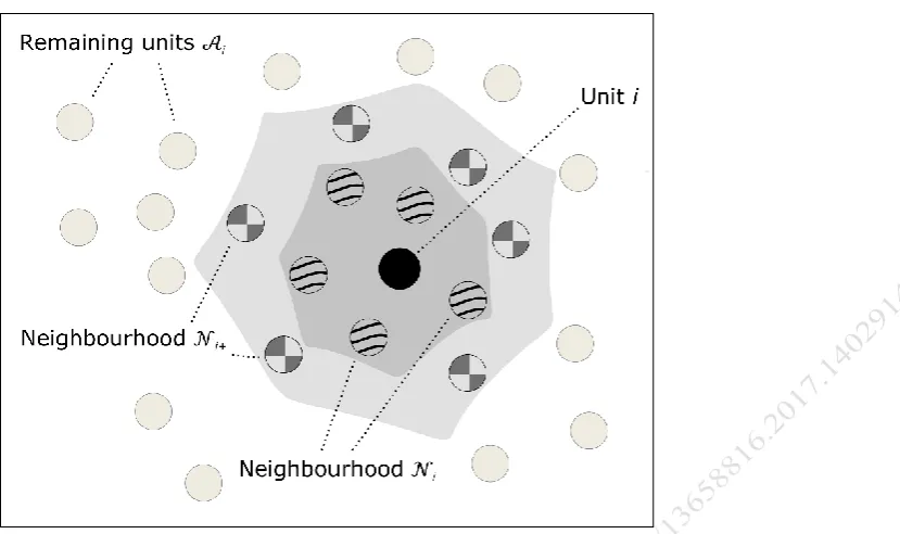
The first stage of the Bayesian predictive approach is to construct a prior that models previous knowledge about the sampling variability of local spatial mean values. The prior must maintain realism, but, at the same time, it should not interfere with the likelihood of the local data that is used in the posterior. That latter likelihood will be obtained from information from the neighbourhood of interest, which must thus then be kept for the updating step. The dual use of data might otherwise lead to a dominant prior that drives the posterior too far, especially with small datasets (Berger 2006, Darnieder 2011, Gelman et al. 2013). The dataset is therefore subsetted. In addition to 𝒩 and 𝒩i, we define
𝒩𝑖+ = {𝑘 ∈ 𝒩 | ∃𝑗 ∈ 𝒩𝑖: 𝑤𝑗𝑘 ≠ 0}, 𝒩𝑖 ⊆ 𝒩𝑖+⊆ 𝒩, (7a)
𝒜𝑖 = 𝒩\𝒩𝑖+. (7b)
Figure 1. Schematic illustration of region 𝒩 separated into 𝒩i, 𝒩i+ and 𝒜i.
Constructing an informed prior requires a priori distributional knowledge. While making the allowance for global non-stationarity, it is not guaranteed that the underlying random variables Xj will be distributed in an identical manner. However, through the central limit theorem and assuming the sample size to be reasonably large, it can be assumed that the spatially weighted mean values 𝑌𝑗 = ∑𝑘∈𝒩𝑗𝑤𝑗𝑘𝑥𝑘⁄∑𝑘∈𝒩𝑗𝑤𝑗𝑘
are approximately normal. We thus have Yj ~ N(𝜇𝑋𝑗, 𝑎𝑗𝜎𝑋2𝑗), where 𝜇Xj and 𝜎X2𝑗 are the unknown expectation and variance of the variates 𝑋𝒩𝑗 (i.e., the variates from 𝒩j). The factor 𝑎𝑗 = ∑𝑘∈𝒩𝑗𝑤𝑗𝑘2⁄𝑊𝑗2 (see Appendix B) reflects the geographic constraints from the spatial weights matrix W. We can ignore this latter constant for the moment but will need it later in the bootstrap.
We seek to predict the parameters 𝜇Xj and 𝜎X2𝑗. It must be remembered that the prior should be backed up by a sufficient amount of data. Instead of estimating the parameters multiple times from small neighbourhoods, our aim is to combine all the information from 𝒜i. Since 𝒜i varies across locations, individual priors must be obtained for each neighbourhood. The combined mean and variance estimators are given by (see Appendix C):
𝑥̅𝑐 =
∑𝑗∈𝒜𝑖𝑛𝑗 ⋅ 𝑥̅𝑗
∑𝑗∈𝒜𝑖𝑛𝑗 and 𝑠𝑐
2 = ∑𝑗∈𝒜𝑖(𝑛𝑗−1)(𝑠𝑗2+𝑥̅𝑗2)
(∑𝑗∈𝒜𝑖𝑛𝑗)−𝑛𝒜𝑖
− 𝑥̅𝑐2. (8)
These estimators account for mutually overlapping spatial neighbourhoods. Variable
𝑛𝒜𝑖 is the cardinality of 𝒜i and subscript c illustrates the combinatorial nature of the
The prior is the product of the two marginal densities of mean and variance outlined above. The mean of Gaussian random variables Yj is itself a normal random variable centred on 𝜇0 = 𝑥̅𝑐 and depends on knowledge of the variance:
𝜇𝑋𝑗| 𝜎𝑋𝑗
2 ~ 𝑁 (𝜇 0, 𝜎0 =
𝜎𝑋𝑗2
𝑛𝑖). (9)
Technical, but non-substantive parameters (i.e., hyperparameters) are indicated by subscript 0. Variable 𝑛𝑖 gives the measurement scale of the neighbourhood i of interest. We use 𝑛𝑖 rather than the scale that is actually associated with x̅c to increase the realism
of the prior. The much larger cardinality of 𝒜i would otherwise cause the prior to be underdispersed. The influence of the prior on predictions could then become overly dominant. Employing ni instead, is a means of matching the prior scale to that of the neighbourhood of interest and is thus more appropriate.
The variance 𝜎𝑋2𝑗 follows a normal scaled inverse-chi-squared distribution
(Gelman et al. 2013, p. 67f.). This results from the χ²-distributed scaled ratio of the sample variance to the variance of the population:
(𝑛𝑖−1)⋅𝑠𝑐2
𝜎𝑋𝑗2 ~𝜒𝑛𝑖−1
2 ⇒ 𝜎 𝑋𝑗
2 ~ 𝜒
𝑠𝑐𝑎𝑙𝑒𝑑−2 (𝜐0, 𝜏02). (10)
As in the case of the mean, the degrees of freedom υ0 is adjusted to ni–1 instead of (∑𝑛𝑖=1𝑛𝑖) − 𝑛, as it is necessary for the prior to be informative about predicting data for
𝒩i rather than 𝒜i. The scale parameter 𝜏02 is equal to the variance estimate 𝑠𝑐2.
A combination of the two marginal densities from Equations (8) and (9) yields the prior (see Appendix D)
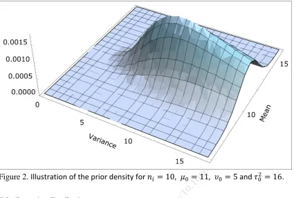
𝜋(𝜇, 𝜎2) ∝ 1
𝜎3+𝑣0 ⋅ exp (−
𝑛𝑖(𝜇−𝜇0)2−𝜐0𝜏02
2𝜎2 ). (11)
Figure 2. Illustration of the prior density for 𝑛𝑖 = 10, 𝜇0 = 11, 𝜐0 = 5 and 𝜏02 = 16.
5.3 Posterior distribution
The posterior combines the prior with the likelihood of the observed local spatial mean value 𝑌𝑖~𝑁(𝜇𝑋𝑖, 𝑎𝑖𝜎𝑋2𝑖). Our aim is to predict suitable values for 𝜇𝑋𝑖 and 𝜎𝑋2𝑖. These parameters specify the final Gaussian from which the additional means are drawn. Constant ai is, again, fixed because it is a non-random property of the neighbourhood of interest. The respective posterior follows a normal scaled inverse-chi-squared distribution and yields (see Appendix E)
𝑓(𝜇𝑋𝑖, 𝜎𝑋𝑖
2 | 𝑌 𝑖) ∝
1 𝜎
𝑋𝑖4+𝜐0
⋅ exp (−𝑛𝑖(𝜇𝑋𝑖−𝜇0)
2
+(𝑌𝑖−𝜇𝑋𝑖) 2
+𝜐0𝜏02
2𝜎𝑋𝑖2 ). (12)
Drawing values for 𝜇𝑋𝑖 and 𝜎𝑋2𝑖 requires deriving the conditional posterior
𝜇𝑋𝑖 | 𝜎𝑋𝑖
2, 𝑌
𝑖 and, since this in turn requires a known 𝜎𝑋𝑖
2, the corresponding marginal
posterior 𝜎𝑋2𝑖 | 𝑌𝑖. By building on the results obtained from Gelman et al. (2013), we derive
𝜇𝑋𝑖 | 𝜎𝑋2𝑖, 𝑌𝑖 ~ 𝑁 (𝜇0+𝑌𝑖
2 ,
𝜎𝑋𝑖2
2𝑛𝑖), (13a)
𝜎𝑋2𝑖 | 𝑌𝑖 ~ 𝜒𝑠𝑐𝑎𝑙𝑒𝑑−2 (𝜐0+ 𝑛𝑖, 𝜏̃2) and 𝜏̃2 = 𝜐0𝜏02+(𝑛𝑖−1)𝑠2+𝑛𝑖2(𝑌𝑖−𝜇0)2
𝜐0+𝑛𝑖 , (13b)
posterior is supported by twice the amount of information, as it is based on two separate mean estimations. The marginal variance posterior in Equation (13b) has additive degrees of freedom, whereas the updated scale parameter 𝜏̃2 combines the prior and
observed sum of squares. The latter are dilated by extra uncertainty from the deviation between the combined means. While the two individual sums of squares in the numerator represent the variability within the individual distributions, the additional uncertainty stems from the likelihood of both occurring together.
Equations (13a) and (13b) demonstrate that the prior and the local information each supply half of the posterior information. The benefit of this is that the posterior is robust against inflation, which might be caused by local boundary conditions or by extreme global imbalance.
5.4 Bootstrapping
The final methodological stage is to generate a bootstrap distribution for LSD that involves the Bayesian procedure outlined above. In each bootstrap iteration, the following steps must be repeated:
(1) random resampling with replacement within the local neighbourhoods, (2) drawing of new synthetic means and recalculation of the residuals,
(3) recalculation of LSD for each drawn pseudo-sample with substituted means, (4) estimation of an empirical distribution of LSD and assessment of pseudo
p-values p*.
These four stages resemble the Monte Carlo approach outlined in (Hope 1968). A concise description of the stages that are usually involved in this kind of approach, is also found in (Dray 2011, p.129f.). What differentiates our approach from these two studies is that the proposed bootstrap is locally constrained. The drawing of additional means in Stage 2 involves the Bayesian approach from Sections (5.2) and (5.3) and is achieved in three phases:
(1) drawing of a posterior variance 𝜎𝑋2𝑖 from Equation (13b),
(2) substitution of 𝜎𝑋2𝑖 into Equation (13a) and drawing of a posterior mean 𝜇 𝑋𝑖,
(3) drawing of new mean values from 𝑁(𝜇𝑋𝑖, 𝑎𝑖𝜎𝑋2𝑖).
The pseudo p-values p* that are needed for inference can then be calculated in different ways, depending on the desired hypothesis testing scheme (Table 1).
Testing scheme Pseudo p-value estimator Interpretation of p*< α
Right-tailed 𝑝∗ = 1
𝑚#{𝑘 | 𝐿𝑆𝐷𝑖𝑘 > 𝐿𝑆𝐷𝑖0} Geographic
arrangement increases the variance
Left-tailed 𝑝∗ = 1
𝑚#{𝑘 | 𝐿𝑆𝐷𝑖𝑘 < 𝐿𝑆𝐷𝑖0} Geographic
arrangement reduces the variance
Two-tailed 𝑝∗ = 1
𝑚#{𝑘 | 𝐿𝑆𝐷𝑖 ∗
𝑘 > 𝐿𝑆𝐷𝑖0},
where 𝐿𝑆𝐷𝑖∗𝑘 = |𝐿𝑆𝐷𝑖𝑘 − 𝐿𝑆𝐷̅̅̅̅̅̅𝑖𝑘|
Geographic
arrangement affects the variance
6. Empirical results from a LiDAR-derived dataset
Figure 3. Height differences between two ATLS datasets.
[image:17.595.86.511.472.732.2]6.1 Interpretation of LSD and LOSH
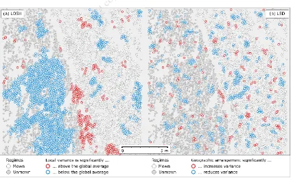
The results from LSD and LOSH reveal different features of variance patterns. Thus, when they are interpreted together, it is easier to make a direct comparison. Figure 4 maps statistically significant LOSH and LSD outcomes. We randomise locally, but omit the Bayesian approach for the moment, as all the involved neighbourhoods are sufficiently large. The smallest available neighbourhood size is ni = 8, which allows 8! = 40,320 permutations. The average of ni = 54, however, allows ca. 2.31 × 1071 permutations, which is enough for virtually all the application scenarios. Despite this, ni = 8 is still a small number of observations and hence contains little information. The Bayesian technique thus proves to be useful, as will be discussed in Sub-section 6.5.
The global dividing line cutting across the centre of the region, is a feature where significant LOSH values from the right tail of the reference distribution accumulate (Figure 4a). Thereby, the southern part dominates, while the northern part of the line is influenced by a spatial gap (a gentle slope in the terrain) which is an obstacle to high LOSH scores. Further high values are found in the mown regime, in particular in the northernmost part (disturbances from artefacts) and in the South (these vanish when the false discovery rate is controlled by following Benjamini and Hochberg (1995)). In contrast, the western unmown part is dominated by significantly low LOSH values. These are caused by the global resampling scheme of LOSH, which shifts statistically differing values from the mown part into the unmown region. This biases the p-values towards the left tail of the bootstrap distribution and makes it impossible to disclose local variance patterns. The eastern mown regime is not as homogeneous as expected. Grass cuttings produced from the lawn mower were being left on the meadow. This increases the global average residual h1 and in turn leads to a more homogeneous appearance of the unmown regime, as explained earlier. Nevertheless, LOSH reveals and maps the global variance structure in the locality by identifying the most (the dividing line) and least dispersed areas (the unmown part).
Table 2. Descriptive statistics for LSD scores within the mown and unmown regimes.
Regime Min Max Mean Median Standard
deviation
Interquartile range
Mown 0.146 3.185 0.907 0.823 0.363 0.446
Unmown 0.249 4.426 0.904 0.782 0.453 0.501
In summary it can be stated that an evaluation of LOSH and LSD scores in combination reveals both global and local variance patterns. The observed LSD values further confirm that, at least for the adjusted analytical scale, the dividing line is a global feature. It is also clear that local structures that remain hidden with LOSH are present in the map when LSD is considered. The LSD scores thus provide an additional insight into the dataset.
6.2 A map of global and local spatial variance patterns
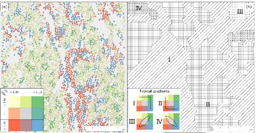
It is worth flagging the significance of the LSD and LOSH values, but they are not exhaustive in terms of their interpretation. The maps in Figure 5 thus provide a classification scheme for LOSH-LSD tuples. Four standard gradients can be derived from these, each characterising different sub-regions in the map.
[image:19.595.87.516.407.628.2]Figure 5 shows a way to classify LOSH and LSD outcomes together. A prominent feature in Figure 5a is, again, the dividing line (see also Type II gradient in Figure 5b). The figure, however, shows the line in more detail: The centre of the line appears to be narrow and elongated and reflects the thin crisp edge of the boundary where the two regimes meet. The spatial pattern strongly increases the variance in this from both a global and local standpoint. Adjoining this is a fuzzy region where local spatial effects are negligible, while the spatial variance is generally high in a global comparison. In other words, while the global variance gradient features prominently, the local spatial variance pattern is closer to randomness and regularity. The local geographic arrangement is thus not related to the increased variance in these regions.
When one moves farther away from the dividing line, the effects prevail at a local level. The variance structures turn into insular regions of small areas where the local pattern increases the variance, which are surrounded by a homogenising geographic arrangement (Type I). The northern part, which is affected by artefacts, is further characterised by two volatile variance patterns (Types III and IV). The Type III pattern, which is featured in the north-eastern part, is caused by a larger haystack. This appears to be regular in local terms (its internal structure), but is disruptive globally as it is a prominent feature (above the global mean variance). In contrast, the Type IV pattern reflects taller bunch grass that is characterised by abrupt fluctuations between regular and heterogeneous conditions caused by the related clumps of culms. An interpretation that combined LOSH and LSD made it possible to distinguish these rather different features in the data.
The detailed interpretations given above, demonstrate the additional value that LSD provides. Global structures are detected and mapped locally by LOSH where these dominate, but local details are missed out. In contrast, LSD assesses local structures and describes in greater detail the internal structure of global features (e.g., the nature of the central boundary or of the homogeneous sub-regions). The measure thus not only assesses different structures, but also reveals additional information about features obtained from LOSH.
6.3 Interplay with variance
Since both LSD and LOSH are measures of variance, it is worth investigating how they relate to the magnitude of the non-spatial local variance. This illustrates the ability of LOSH and LSD to separate effects of spatial patterning from other influences of general variability.
(Koenker and Bassett 1982, Godfrey 1996) on the residuals, confirms the heteroscedasticity that is visible in Figure 6a. The two diverging quartile trend lines in the biquantile regressogram (Figure 6b) underpin this outcome, while the median trace shows that variance is a good predictor of LOSH. The measure is thus dominated by non-spatial variability. This result is in accordance with the intended purpose of LOSH to detect both the most and least dispersed regions in geographic data. However, it also shows that LOSHs power to detect solely spatial effects in local circumstances is limited.
Figure 6. Relationship between LOSH and local variance. (a) A scatter plot of variance and LOSH; and (b) A biquantile regressogram (Tukey 1977) illustrating heteroscedasticity in LOSH.
Figure 7. Relationship between LSD and local variance. (a) A scatter plot of variance with regard to LSD; and (b) a biquantile regressogram (Tukey 1977) illustrating heteroscedasticity within LSD.
Figure 8. The relationship of LOSH and LSD with local Moran’s I. The logarithms of the two measures were chosen to improve interpretability. The red line represents a first-order LOESS trend. (a) LOSH; and (b) LSD.
6.4 Relationship with spatial autocorrelation
[image:22.595.87.516.67.276.2] [image:22.595.87.510.328.555.2]highlight similar structures from different perspectives (variance vs. covariance). Observations showing autocorrelations higher than 1.4 belong to the northern artefacts and thus can reasonably be regarded as outliers, that do not conform to the general observations made above. Overall, LOSH reveals roughly similar structures to those of Moran’s I, as is evident from their antipodal behavioural pattern.
[image:23.595.85.512.280.711.2]In contrast, LSD is almost unrelated to Moran’s I, when the latter is on the interval [0.0, 1.4]. Most of the data points accumulate on the left side of the scatter plot in Figure 8b without showing any notable trend (τ = -0.09). This strengthens the likelihood indicated above that LSD is able to reveal patterns that cannot be detected by LOSH and Moran’s I. These detected patterns are not linked to the clustering tendency of the attribute values. Rather, they are features in their own right, which makes them of value for empirical investigations since they might supply important details about the disclosure of the mechanisms in spatial random variables.
6.5 Influence of the Bayesian prediction of mean values
The Bayesian procedure from Section 5 extends local resampling by the use of synthetic data generated from empirical prior knowledge combined with local information. This approach differs from conventional bootstrapping that only relies on observed information. There is a need to investigate how the Bayesian approach influences drawn inferences.
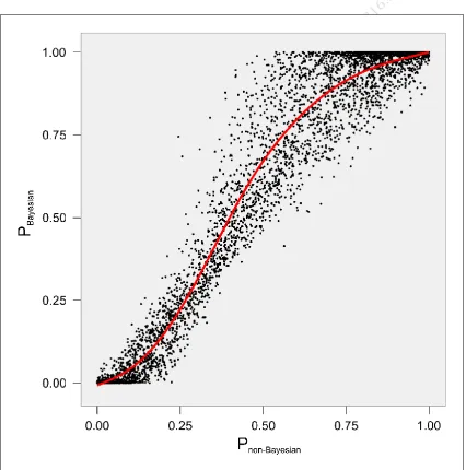
Figure 9 shows a sigmoidal relationship between conventional p-values (i.e., those that were used in the previous paragraphs) and those involving synthetic means. They show a strong monotonic association of τ = 0.77 at medium ranges. There is a significant fall in this association in both tails (τ = 0.23), which is an important observation as the tails possess values which are important for drawing inferences. In the Bayesian approach, the p-values tend to concentrate around the extremes of 0 and 1. In contrast, conventional p-values show a higher level of dispersion in the tails. This is caused by the number of available observations, which have limited explanatory power because they only represent a small fraction of all possible values. In contrast, the Bayesian approach extends this spectrum, which increases its ability to detect spatial effects because the comparative values are not biased towards a certain range.
The increased ability to detect effects with the Bayesian approach is further evident after the p-values have been corrected for multiple hypothesis testing. Note that LSD tests n hypotheses with one dataset. This repeated use of the data leads to an increase in the Type I error rate and requires correction. When the false-discovery rate is controlled at α = 0.05 (FDR; Benjamini and Hochberg 1995) and the p-values are corrected accordingly, it is seen that the non-Bayesian approach is very conservative. Only 0.5% of all the null hypotheses are rejected, which is way below the significance level that was envisaged. In other words, many actual effects might be missed out. In contrast, when the Bayesian-generated p-values are adjusted, they yield a ratio of 5.2%, which is close to the desired α level.
Figure 10 illustrates the FDR-corrected p-values of significant observations by incorporating the Bayesian-generated means. The significant features in the eastern part (the ‘mown’) show a general North-South bearing (Figure 10a) and resemble the direction of the mowing process, which is illustrated in the background of Figure 10b through a hill-shading raster. The blue features, where the geographic layout reduces the variance, either accumulate alongside the small piles of hay that were left on the meadow or in the furrows in-between. In contrast, the western part (the ‘unmown’) is not affected by the after-mowing topography. The patterns of significant features observed in this part are mostly unrelated to the hill-shading. This makes sense given that the height differences that were analysed are affected by physical, biological and other factors that do not necessarily correspond to the topography shown in Figure 10b, especially in the unmown area.
phenomenon (especially in the mown part) and can thus be considered to be of greater value. Hence, this comparison implies that the proposed Bayesian approach is a reasonable alternative to more conventional forms of pseudo p-value estimation.
Figure 10. Significant LSD scores involving Bayesian-predicted means (two-sided test;
α = 0.05; 1,000 iterations). (a) Map of significant features. (b) Schematic sketch of significant accumulated features, against the background of the hill-shading of the surface after the mowing.
7. Discussion and conclusions
This paper introduces a test called ‘Local Spatial Dispersion’ (LSD), which is able to determine the local influence of geographic arrangements on variance. It does not incorporate global information and allows local patterns to be detected in the presence of a global structure. The strictly local nature of the test, however, increases the risk of problems arising from small-size samples within local neighbourhoods. To mitigate this risk, a stratified bootstrapping procedure is introduced that combines traditional resampling with a Bayesian prediction of synthetic data. The proposed LSD supplements LOSH, which is a recently devised technique to map global variance structures locally. The measure adapts LOSH to strictly local circumstances. Conceptually, LSD forms a part of a series of localised techniques like the hot spot method called ‘O-statistic’ (Ord and Getis 2001), or locally adaptive geometric clustering techniques such as the inhomogeneous marked and unmarked K-functions (Cuzick and Edwards 1990, Baddeley et al. 2000).
Furthermore, the obtained results show that LOSH is closely correlated with general non-spatial variability, which hampers the separation of genuinely spatial from other effects. In contrast, LSD is uncorrelated with non-spatial variation and is capable of exposing entirely spatial variance effects. Notably, LSD is also unrelated to positive spatial autocorrelation. This allows the measure to assess other complex patterns apart from general attribute clustering, such as the internal structures of clusters and the detailed contours of geographic boundaries. The proposed inference mechanism further facilitates the detection of local structures. While conventional stratified bootstrapping turns out to be overly conservative, the synthetic expansion of the available local data keeps the α-rate in compliance with the adjusted significance level, which increases its ability to detect meaningful patterns. Overall, LSD has been shown to be a useful extension to the spatial analysis toolbox. In the given example, it is possible, in statistical terms, to detect local interaction between variance and spatial patterns within global structures and thus to disclose details that would otherwise have been overlooked.
The anonymous reviewers pointed out that there was a relationship between the proposed LSD technique and local variograms. Variograms quantify the variance of the spatial increment between two locations separated by a certain distance (Bachmaier and Backes 2008, Cuba et al. 2012). Both, LSD and variograms are thus concerned with variance estimation. What differentiates them is that LSD is a) a hypothesis test designed to determine the influence of a specific spatial arrangement on variance and b) that it is concerned with in-place variance rather than with the variance of the incremental process. In contrast, variograms estimate variance within certain distance bands by relying on the validity of the employed spatial weights (instead of testing their influence). The estimates of the variograms are then used for modelling (e.g., in Kriging), which means that our proposed test can be used as a diagnostic tool for geostatistics. For instance, LSD can be used to fully investigate the possible sources of local non-stationarities, which might lead to a lack of stationarity in the difference processes between locations. Thus, LSD might also be a useful device in the area of geostatistics.
robust for inhomogeneous populations and assist its interpretation. From a technological standpoint, the proposed solution is computationally expensive as it includes bootstrapping. The application of LSD to large datasets would hence clearly benefit from an efficient implementation strategy. All in all, LSD provides the means of obtaining a valuable and detailed insight into variance mechanisms of geographic random variables and offers the prospect of achieving significant new empirical results in various fields.
Acknowledgements
This work was supported by the German Research Foundation (DFG) through the priority programme ‘Volunteered Geographic Information: Interpretation, Visualisation and Social Computing’ (SPP 1894). Special thanks go to Prof Thomas Glade (University of Vienna) for the provision of LiDAR data from the ‘4DEMON’ project. We would also like to thank the Lower Austrian government for their financial support for the LiDAR data collection within the framework of the ‘NoeSLIDE’ project.
References
Abascal, M. and Baldassarri, D., 2015. Love Thy Neighbor? Ethnoracial Diversity and Trust Reexamined. American Journal of Sociology, 121 (3), 722–782.
Anderson, C., Lee, D., and Dean, N., 2014. Identifying Clusters in Bayesian Disease Mapping. Biostatistics, 15 (3), 457–469.
Anselin, L., 1988. Lagrange Multiplier Test Diagnostics for Spatial Dependence and Spatial Heterogeneity. Geographical Analysis, 20 (1), 1–17.
Anselin, L., 1990. Spatial Dependence and Spatial Structural Instability in Applied Regression Analysis. Journal of Regional Science, 30 (2), 185–207.
Anselin, L., 1995. Local Indicators of Spatial Association - LISA. Geographical Analysis, 27 (2), 93–115.
Anselin, L., 2001. Spatial Econometrics. In: B. Baltagi, ed. A Companion to Theoretical Econometrics. Hoboken, NJ: Wiley-Blackwell, 310–330.
Anselin, L., 2010. Thirty Years of Spatial Econometrics. Papers in Regional Science, 89 (1), 3–25.
Arnot, C. and Fisher, P., 2007. Mapping the Ecotone with Fuzzy Sets. In: A. Morris and S. Kokhan, eds. Geographic Uncertainty in Environmental Security. Dordrecht: Springer Netherlands, 19–32.
Bachmaier, M. and Backes, M., 2008. Variogram or Semivariogram? Understanding the Variances in a Variogram. Precision Agriculture, 9, 173–175.
Baddeley, A., Moller, J., and Waagepetersen, R., 2000. Non- and Semi-Parametric Estimation of Interaction in Inhomogeneous Point Patterns. Statistica Neerlandica, 54 (3), 329–350.
Barbujani, G., Oden, N., and Sokal, R., 1989. Detecting Regions of Abrupt Change in Maps of Biological Variables. Systematic Zoology, 38 (4), 376–389.
Terrestrial Laser Scanning, Selawik River, Alaska. Remote Sensing, 5 (6), 2813– 2837.
Bavaud, F., 2014. Spatial weights: constructing weight-compatible exchange matrices from proximity matrices. In: M. Duckham, E. Pebesma, K. Stewart, and A.U. Frank, eds. Geographic Information Science: 8th International Conference, GIScience 2014. Vienna, Austria: Springer Berlin Heidelberg, 81–96. Benjamini, Y. and Hochberg, Y., 1995. Controlling the False Discovery Rate : A
Practical and Powerful Approach to Multiple Testing. Journal of the Royal Statistical Society: Series B (Methodological), 57 (1), 289–300.
Berger, J., 2006. The Case for Objective Bayesian Analysis. Bayesian Analysis, 1 (3), 385–402.
Berkes, F., Hughes, T., Steneck, R., Wilson, J., Bellwood, D., Crona, B., Folke, C., Gunderson, L., Leslie, H., Norberg, J., Nyström, M., Olsson, P., Österblom, H., Scheffer, M., and Worm, B., 2006. Globalization, Roving Bandits, and Marine Resources. Science, 311 (5767), 1557–1558.
Box, G., 1953. Non-Normality and Tests on Variances. Biometrika, 40 (3/4), 318–335. Bravo, C. and Weber, R., 2011. Semi-Supervised Constrained Clustering with Cluster
Outlier Filtering. In: C. San Martin and S. Kim, eds. Progress in Pattern Recognition, Image Analysis, Computer Vision, and Applications. Heidelberg: Springer, 347–354.
Brunsdon, C., Fotheringham, S., and Charlton, M., 1998. Geographically Weighted Regression. Journal of the Royal Statistical Society: Series D (The Statistician), 47 (3), 431–443.
Cadenasso, M., Pickett, S., and Schwarz, K., 2007. Spatial Heterogeneity in Urban Ecosystems: Reconceptualizing Land Cover and a Framework for Classification. Frontiers in Ecology and the Environment, 5 (2), 80–88.
Canli, E., Höfle, B., Hämmerle, M., Thiebes, B., and Glade, T., 2015. Permanent 3D Laser Scanning System for an Active Landslide in Gresten (Austria). In:
Geophysical Research Abstracts EGU General Assembly. 2885.
Cochran, W., 1934. The Distribution of Quadratic Forms in a Normal System, with Applications to the Analysis of Covariance. Mathematical Proceedings of the Cambridge Philosophical Society, 30 (2), 178–191.
Csillag, F. and Sándor, K., 2002. Wavelets, Boundaries, and the Spatial Analysis of Landscape Pattern. Écoscience, 9 (2), 177–190.
Cuba, M., Leuangthong, O., and Ortiz, J., 2012. Detecting and Quantifying Sources of Non-Stationarity via Experimental Semivariogram Modeling. Stochastic
Environmental Research and Risk Assessment, 26 (2), 247–260.
Cuzick, J. and Edwards, R., 1990. Spatial Clustering for Inhomogeneous Populations. Journal of the Royal Statistical Society . Series B (Methodological), 52 (1), 73– 104.
Darnieder, W., 2011. Bayesian Methods for Data-Dependent Priors. Columbus, OH: The Ohio State University.
Dutilleul, P., 2011. Spatio-Temporal Heterogeneity: Concepts and Analyses. Cambridge, UK: Cambridge University Press.
Dutilleul, P. and Legendre, P., 1993. Spatial Heterogeneity Against Heteroscedasticity: An Ecological Paradigm Versus a Statistical Concept. Oikos, 66 (1), 152–171. Fagan, W., Cantrell, R., and Cosner, C., 1999. How Habitat Edges Change Species
Interactions. The American Naturalist, 153 (2), 165–182.
Fagan, W., Fortin, M., and Soykan, C., 2003. Integrating Edge Detection and Dynamic Modeling in Quantitative Analyses of Ecological Boundaries. BioScience, 53 (8), 730.
Fang, H. and Huang, D., 2004. Noise Reduction in LiDAR Signal Based on Discrete Wavelet Transform. Optics Communications, 233 (1–3), 67–76.
Fisher, P. and Robinson, V., 2014. Fuzzy Modelling. In: R. Abrahart and L. See, eds. GeoComputation. Boca Raton, FL: CRC Press, 283–306.
Forman, R., 1995. Land Mosaics: The Ecology of Landscapes and Regions. Cambridge, UK: Cambridge University Press.
Fortin, M., 1994. Edge Detection Algorithms for Two-Dimensional Ecological Data. Ecology, 75 (4), 956–965.
Fortin, M., 1999. Spatial Statistics in Landscape Ecology. In: J. Klopatek and R.
Gardner, eds. Landscape Ecological Analysis. New York, NY: Springer, 253–279. Fotheringham, A., Charlton, M., and Brunsdon, C., 1996. The Geography of Parameter
Space: An Investigation of Spatial Non-Stationarity. International Journal of Geographical Information Systems, 10 (5), 605–627.
Fotheringham, A.S., Brunsdon, C., and Charlton, M., 2002. Geographically weighted regression: the analysis of spatially varying relationships. Chichester: John Wiley & Sons.
Gaetan, C. and Guyon, X., 2010. Spatial statistics and modelling. New York, NY: Springer.
Garrigues, S., Allard, D., Baret, F., and Weiss, M., 2006. Quantifying Spatial
Heterogeneity at the Landscape Scale Using Variogram Models. Remote Sensing of Environment, 103 (1), 81–96.
Gelfand, A. and Banerjee, S., 2015. Bayesian Wombling: Finding Rapid Change in Spatial Maps. Wiley Interdisciplinary Reviews: Computational Statistics, 7 (October), 307–315.
Gelman, A., Carlin, J., Stern, H., Dunson, D., Vehtari, A., and Rubin, D., 2013. Bayesian Data Analysis. 3rd ed. Boca Raton, FL: CRC Press.
Getis, A., 2010. Spatial Autocorrelation. In: M. Fischer and A. Getis, eds. Handbook of Applied Spatial Analysis. Heidelberg: Springer, 255–278.
Getis, A., 2015. Analytically Derived Neighborhoods in a Rapidly Growing West African City: The Case of Accra, Ghana. Habitat International, 45 (Part 2), 126– 134.
Getis, A. and Ord, J., 1992. The Analysis of Spatial Association by Use of Distance Statistics. Geographical Analysis, 24 (3), 189–206.
Goovaerts, P., 2008. Accounting for Rate Instability and Spatial Patterns in the Boundary Aanalysis of Cancer Mortality Maps. Environmental and Ecological Statistics, 15 (4), 421–446.
Goovaerts, P., 2010. How do Multiple Testing Correction and Spatial Autocorrelation Affect Areal Boundary Analysis? Spatial and Spatio-temporal Epidemiology, 1 (4), 219–229.
Graif, C. and Sampson, R., 2009. Spatial Heterogeneity in the Effects of Immigration and Diversity on Neighborhood Homicide Rates. Homicide Studies, 13 (3), 242– 260.
Grillet, M., Jordan, G., and Fortin, M., 2010. State Transition Detection in the Spatio-Temporal Incidence of Malaria. Spatial and Spatio-temporal Epidemiology, 1 (4), 251–259.
Hanson, T., Banerjee, S., Li, P., and McBean, A., 2015. Spatial Boundary Detection for Areal Counts. In: R. Mitra and P. Müller, eds. Nonparametric Bayesian Inference in Biostatistics. New York, NY: Springer, 377–399.
Höfle, B., Canli, E., Schmitz, E., Crommelinck, S., and Hoffmeister, D., 2016. 4D Near Real-Time Environmental Monitoring Using Highly Temporal LiDAR. In:
Geophysical Research Abstracts of the EGU General Assembly.
Hope, A., 1968. A Simplified Monte Carlo Significance Test Procedure. Journal of the Royal Statistical Society. Series B (Methodological), 30 (3), 582–598.
Hu, T., Liu, Q., Du, Y., Li, H., and Huang, H., 2015. Analysis of Land Surface Temperature Spatial Heterogeneity Using Variogram Model. In: IEEE
International Geoscience and Remote Sensing Symposium 2015. Milan: IEEE, 132–135.
Hungr, O., Leroueil, S., and Picarelli, L., 2014. The Varnes Classification of Landslide Types, an Update. Landslides, 11 (2), 167–194.
Jaboyedoff, M., Oppikofer, T., Abellán, A., Derron, M., Loye, A., Metzger, R., and Pedrazzini, A., 2012. Use of LiDAR in Landslide Investigations: A Review. Natural Hazards, 61 (1), 5–28.
Jacquez, G., 2010. Geographic Boundary Analysis in Spatial and Spatio-Temporal Epidemiology: Perspective and Prospects. Spatial and Spatio-Temporal Epidemiology, 1 (4), 207–218.
Jacquez, G., Kaufmann, A., and Goovaerts, P., 2008. Boundaries, Links and Clusters: A New Paradigm in Spatial Analysis? Environmental and Ecological Statistics, 15 (4), 403–419.
Jacquez, G., Maruca, S., and Fortin, M., 2000. From Fields to Objects: A Review of Geographic Boundary Analysis. Journal of Geographical Systems, 2 (3), 221–241. Jiang, B., 2015. Geospatial Analysis Requires a Different Way of Thinking: The
Problem of Spatial Heterogeneity. GeoJournal, 80 (1), 1–13.
Keitt, T. and Urban, D., 2005. Scale-Specific Inference Using Wavelets. Ecology, 86 (9), 2497–2504.
Kent, M., Gill, W., Weaver, R., and Armitage, R., 1997. Landscape and Plant
Kent, M., Moyeed, R., Reid, C., Pakeman, R., and Weaver, R., 2006. Geostatistics, Spatial Rate of Change Analysis and Boundary Detection in Plant Ecology and Biogeography. Progress in Physical Geography, 30 (2), 201–231.
Koenker, R. and Bassett, G., 1982. Robust Tests for Heteroscedasticity Based on Regression Quantiles. Econometrica, 50 (1), 43–61.
Kolasa, J. and Rollo, C., 1991. The Heterogeneity of Heterogeneity: A Glossary. In: J. Kolasa and S. Pickett, eds. Ecological Heterogeneity. Heidelberg: Springer, 1–23. Lague, D., Brodu, N., and Leroux, J., 2013. Accurate 3D Comparison of Complex
Topography with Terrestrial Laser Scanner: Application to the Rangitikei Canyon (N-Z). ISPRS Journal of Photogrammetry and Remote Sensing, 82, 10–26.
Laurance, W., Didham, R., and Power, M., 2001. Ecological Boundaries: A Search for Synthesis. Trends in Ecology & Evolution, 16 (2), 70–71.
Lee, D. and Mitchell, R., 2012. Boundary Detection in Disease Mapping Studies. Biostatistics, 13 (3), 415–426.
Legewie, J. and Schaeffer, M., 2016. Contested Boundaries: Explaining Where Ethno-Racial Diversity Provokes Neighborhood Conflict. American Journal of Sociology, 122 (1), 125–161.
Lillesand, T., Kiefer, R., and Chipman, J., 2015. Remote Sensing and Image Interpretation. 7th ed. Hoboken, NJ: Wiley & Sons.
Lohrer, A., Rodil, I., Townsend, M., Chiaroni, L., Hewitt, J., and Thrush, S., 2013. Biogenic Habitat Transitions Influence Facilitation in a Marine Soft-Sediment Ecosystem. Ecology, 94 (1), 136–145.
Lovelace, R., Birkin, M., Cross, P., and Clarke, M., 2016. From Big Noise to Big Data: Toward the Verification of Large Data Sets for Understanding Regional Retail Flows. Geographical Analysis, 48 (1), 59–81.
Mandelbrot, B. and Hudson, R., 2004. The (Mis)behavior of Markets: A Fractal View of Risk, Ruin, and Reward. New York, NY: Basic Books.
Ord, J. and Getis, A., 1995. Local Spatial Autocorrelation Statistics: Distributional Issues and an Application. Geographical Analysis, 27 (4), 286–306.
Ord, J. and Getis, A., 2012. Local Spatial Heteroscedasticity (LOSH). The Annals of Regional Science, 48 (2), 529–539.
Ord, J.K. and Getis, A., 2001. Testing for local spatial autocorrelation in the presence of global autocorrelation. Journal of Regional Science, 41 (3), 411–432.
Páez, A. and Scott, D.M., 2004. Spatial statistics for urban analysis : A review of techniques with examples. GeoJournal, 61, 53–67.
Patil, G., Modarres, R., Myers, W., and Patankar, P., 2006. Spatially Constrained Clustering and Upper Level Set Scan Hotspot Detection in Surveillance Geoinformatics. Environmental and Ecological Statistics, 13 (4), 365–377.
Perkins, T., Scott, T., Le Menach, A., and Smith, D., 2013. Heterogeneity, Mixing, and the Spatial Scales of Mosquito-Borne Pathogen Transmission. PLOS
Computational Biology, 9 (12), e1003327.
Conference on Advances in Geographic Information Systems (SIGSPATIAL’13). Orlando, FL: ACM, 264–273.
Sparrow, A., 1999. A Heterogeneity of Heteogeneities. Trends in Ecology & Evolution, 14 (11), 422–423.
Steiger, E., Resch, B., and Zipf, A., 2016. Exploration of spatiotemporal and semantic clusters of Twitter data using unsupervised neural networks. International Journal of Geographical Information Science, 30 (9), 1694–1716.
Strayer, D., Power, M., Fagan, W., Pickett, S., and Belnap, J., 2003. A Classification of Ecological Boundaries. BioScience, 53 (8), 723–729.
Tian, P., Cao, X., Liang, J., Zhang, L., Yi, N., Wang, L., and Cheng, X., 2014. Improved Empirical Mode Decomposition Based Denoising Method for LiDAR Signals. Optics Communications, 325, 54–59.
Tukey, J., 1977. Exploratory Data Analysis. Boston, MA: Addison-Wesley.
Turner, M., 1989. Landscape Ecology: the Effect of Pattern on Process. Annual Review of Ecology and Systematics, 20 (1), 171–197.
Wagner, H. and Fortin, M., 2005. Spatial Analysis of Landscapes: Concepts and Statistics. Ecology, 86 (8), 1975–1987.
Walck, C., 2007. Hand-Book on Statistical Distributions for Experimentalists. Stockholm: University of Stockholm.
Wang, J., Zhang, T., and Fu, B., 2016. A Measure of Spatial Stratified Heterogeneity. Ecological Indicators, 67, 250–256.
Womble, W., 1951. Differential Systematics. Science, 114 (2961), 315–322. Xu, M., Mei, C., and Yan, N., 2014. A Note on the Null Distribution of the Local
Spatial Heteroscedasticity (LOSH) Statistic. The Annals of Regional Science, 52 (3), 697–710.
Ye, X., Wang, T., Skidmore, A., Fortin, D., Bastille-Rousseau, G., and Parrott, L., 2015. A Wavelet-Based Approach to Evaluate the Roles of Structural and Functional Landscape Heterogeneity in Animal Space Use at Multiple Scales. Ecography, 38 (7), 740–750.
Appendix A: Relationship between LOSH and LSD
The ratio between LOSH and LSD is given by
𝐻𝑖 𝐿𝑆𝐷𝑖 =
1
𝑛𝑖∑ |𝑒𝑗| 2
𝑗∈𝒩𝑖 ⋅ ∑ 𝑤𝑖𝑗|𝑒𝑗|
2
𝑗∈𝒩 ⋅ ∑𝑗∈𝒩𝑤𝑖𝑗
1
𝑛∑ |𝑒𝑗| 2
𝑗∈𝒩 ⋅ ∑ 𝑤𝑖𝑗|𝑒𝑗|
2
𝑗∈𝒩 ⋅ ∑𝑗∈𝒩𝑤𝑖𝑗
= 𝑛 ⋅ ℎ𝑖
∑𝑗∈𝒩|𝑒𝑗|2 = ℎ𝑖 ⋅ ℎ1 −1.
From this, LOSH and LSD can be inferred: 𝐻𝑖 = 𝐿𝑆𝐷𝑖 ⋅ ℎ𝑖
ℎ1 and 𝐿𝑆𝐷𝑖 =
𝐻𝑖 ⋅ ℎ1
ℎ𝑖 .