NCSU SAS Ning: Candidate Generation and Feature Engineering for Supervised Lexical Normalization

NCSU-SAS-Ning: Candidate Generation and Feature Engineering for

Supervised Lexical Normalization

Ning Jin

Text Analytics R&D

SAS Institute, Inc.

Cary, NC, USA

[email protected]

Abstract

User generated content often contains non-standard words that hinder effective automatic text processing. In this paper, we present a system we developed to per-form lexical normalization for English Twitter text. It first generates candidates based on past knowledge and a novel string similarity measurement and then selects a candidate using features learned from training data. The system has a con-strained mode and an unconcon-strained mode. The constrained mode participated in the W-NUT noisy English text normal-ization competition (Baldwin et al., 2015) and achieved the best F1 score.

1

Introduction

User generated content, such as customer re-views, forum discussions, text messages and Twitter text, is of great value in applications like understanding users, trend discovery and crowdsourcing. For example, by reading the Twitter text posted by a user, a company can learn the user’s preferences and connections and use the information for targeted advertising. For another example, by reading Amazon customer reviews about a certain product, a shopper can collect a lot of product information that is not available from manufacturers and retailers. Un-fortunately, user generated content often contains ungrammatical sentence structures and non-standard words, which hinders automated text processing.

In this paper, we present a solution that at-tempts to perform lexical normalization (Han et al., 2011) for English Twitter text based on

train-ing text with human annotation (Baldwin et al., 2015). The solution has a constrained mode and an unconstrained mode. Both modes have the same architecture and components. Both use the annotated training data and CMU’s ark POS tag-ger (Gimpel et al., 2011). The difference between them is parameter settings and the usage of a ca-nonical lexicon dictionary by the unconstrained mode.

This paper is organized as follows: Section 2 describes the architecture and components shared by the constrained and unconstrained modes. Section 3 lists what resources are used by each system. In Section 4, we describe the different settings of the constrained and unconstrained modes and compare their performance. Section 5 concludes the paper and discusses future work.

2

Architecture and Components of the

System

Given a tokenized English tweet T = (t1, t2, …,

tn), where ti is the i-th token and n is the total number of tokens, our normalization system pro-cesses one token at a time and has two compo-nents: candidate generation and candidate evalu-ation. To normalize token ti, the system first gen-erates a small set of candidate canonical forms. Then it calculates a confidence score for each candidate and selects the one with the highest confidence score as the canonical form of token ti. How to generate candidates and how to calcu-late confidence scores are learned from training data.

2.1 Candidate Generation The candidates of a token ti include:

• The token itself

• All tokens that are considered canonical

forms of ti in the training data (static map-ping dictionary)

• A split into multiple canonical forms if the

token ti is not a canonical form (for exam-ple, “loveyourcar” à “love your car”)

• Top-m most similar canonical forms found

in training data (see subsection 2.2 for de-tails of similarity measurement)

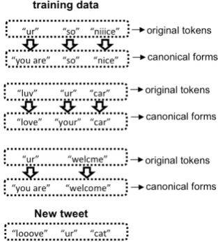
Figure 1 shows an example of training data and a new tweet for normalization. Table 1 shows a portion of the static mapping dictionary learned from the training data.

For token “ur” in the new tweet, the token it-self is “ur”. All of its possible canonical forms present in the training data are “you are” and “your”. Let m = 1, the most similar canonical form is “your”. Therefore, the candidates of “ur” include “ur”, “you are” and “your”. For token “looove” in the new tweet, the token itself is “looove”. It is absent in the training data, so it does not have its own canonical form available as candidates. Among all the canonical forms present in training data, canonical form “love” is most similar to “looove”. Therefore, the candi-dates of “looove” include “looove” and “love”.

Figure 1: An Example of Training Data and a New Tweet for Normalization

Key (token) Value (canonical forms) “ur” “your”, “you are”

“so” “so”

“niiice” “nice”

“luv” “love”

“car” “car”

“welcme” “welcome”

Table 1: Static Mapping Dictionary Learned from Training Data

2.2 Similarity Index

We measure similarity between two strings by first representing each string with a set of simi-larity features and then evaluating simisimi-larity with Jaccard Index (Levandowsky et al., 1971) of the two similarity feature sets.

The similarity features of a string s include n -grams and k-skip-n-grams in s. In this paper, an n-gram in string s is defined as a contiguous se-quence of n characters in s. A k-skip-n-gram in string s is a generalization of n-gram with gaps between characters and is defined as a sequence of n characters where the maximum distance be-tween two characters is k. We prepend (append) a “$” to n-grams that appear at the beginning (end) of the string. We use “|” to indicate gaps in skip-grams. For example, Table 2 shows the sim-ilarity feature sets of “love”, “looove”, “car” and “cat”, with n=2 and k=1.

String Similarity Feature Set “love” “$lo”, “ov”, “ve$”, “l|v”, “o|e”

“looove” “$lo”, “oo”, “ov”, “ve$”, “l|o”, “o|o”, “o|v”, “o|e” “car” “$ca”, “ar$”, “c|r”

“cat” “$ca”, “at$”, “c|t”

Table 2: An Example of Similarity Features (n=2, k=1)

Let the similarity feature set of a string s be f(s), then we measure string similarity between s1 and s2 by:

𝑠𝑖𝑚𝑖𝑙𝑎𝑟𝑖𝑡𝑦 𝑠_!,𝑠_!

=𝐽𝑎𝑐𝑐𝑎𝑟𝑑𝐼𝑛𝑑𝑒𝑥 𝑓 𝑠! ,𝑓 𝑠!

=|𝑓(𝑠!)∩𝑓(𝑠!)|

|𝑓(𝑠!)∪𝑓(𝑠!)|

For example, in Table 2, “love” and “looove” share similarity features {“$lo”, “ov”, “ve$”, “o|e”}. The union of their similarity feature sets is {“$lo”, “oo”, “ov”, “ve$”, “l|v”, “l|o”, “o|o”, “o|v”, “o|e”}. The similarity score between “love” and “looove” is 4/9 = 0.44.

Different weights can be assigned to different similarity features when calculating similarity scores because n-grams at different positions have different importance for word recognition (White et al., 2008). For example, in the example shown in Table 2, we can assign weight 3 to bi-grams at the beginning and end of strings and weight 1 to other features, and then the similarity score between “love” and “looove” becomes 8/13 = 0.615.

and 2-skip-bigrams together. If k = 0, it means no skip-gram is used.

This similarity measurement penalizes text ed-its such as insertion, deletion and substitution. Compared with Levenshtein distance (Le-venshtein, 1966), one disadvantage of our simi-larity measurement is that two different strings may have 1.0 similarity score because the simi-larity feature set can only capture local character order information. For example, strings “aaabaa” and “aaaabaa” have exactly the same similarity feature set {“$aa”, “ab”, “ba”, “aa$”, “a|a”, “a|b”, “b|a”} and thus have 1.0 similarity score. Includ-ing skip-gram and usInclud-ing a larger n in similarity feature calculation can mitigate this problem but cannot prevent it. Fortunately, this should be very rare when the similarity measurement is applied to two real world twitter tokens because such cases require the strings to be long and con-tain repetitive n-grams and skip-grams. One ad-vantage of our similarity measurement over Le-venshtein distance is that it takes into account the string length when penalizing text edits. The same text edit has a bigger impact when it occurs in a short string than in a long string because of the denominator in Jaccard Index. Another ad-vantage of our similarity measurement is that it better handles repetition characters, which is commonly used in Twitter. For example, for our similarity measurement, both “looove” and “loooooove” are equally similar to “love”. For Levenshtein distance, “loooooove” takes a much heavier penalty than “looove”.1 _{The biggest} ad-vantage of our similarity measurement over Le-venshtein distance is the lower computational complexity. Let the length of a string s be l(s). The feature set size of s is bounded by O(l(s)). Then the complexity of calculating Levenshtein distance between s1 and s2 is O(l(s1)l(s2)), which is quadratic when two strings have similar length. On the contrary, the complexity of calcu-lating our similarity measurement is O(l(s1)+l(s2)), which is linear.2

We index all the canonical forms in the train-ing data based on similarity features to facilitate

1 _{Certain preprocessing can mitigate this problem for} Le-venshtein distance. For example, all single character repeti-tions get reduced to two before Levenshtein distance is cal-culated. But it does not handle repetition of multiple charac-ters, e.g. “lolol”.

2 _{The linear complexity depends on using hash table to} cal-culate set union and intersection. Another implementation is sorting the similarity features first and then calculating un-ion and intersectun-ion, which has O(l*log(l)) complexity (l is the longer string length of the two strings) and is still better than quadratic complexity of Levenshtein distance.

finding top-m canonical forms that are most similar to the query token. Given a query token, we can quickly narrow down our search space to canonical forms that share at least one similarity feature with the query token. Further efficiency improvement can be achieved by approximating the denominator in Jaccard Index based on string lengths or by imposing restrictions on the mini-mum number of similarity features to be shared by query token and results.

2.3 Candidate Evaluation

Given a tweet T, one of its token ti and one of the token’s candidate c, we train a binary classifier that predicts whether c is the correct canonical form of ti in the tweet T and outputs a confidence score for the prediction. Among the candidates that the classifier predicts to be the correct ca-nonical forms, we select the one with the highest confidence score as the canonical form of ti. In our implementation of the system, we used a random forest classifier (Breiman, 2001) mainly because its training speed is faster and its per-formance is relatively insensitive to parameter values, but other binary classification algorithm should also work.

This step is mostly feature engineering and we used the following features:

• Support and confidence

We calculate the support of token ti (number of times ti appears) and confidence of token ti being normalized to candidate c (percentage of times ti is normalized to c) according to training data and use them as features for classification. For example, in the training da-ta shown above, the support of token “ur” is 3 and the confidence of normalizing “ur” to “you are” is 2/3 = 0.67. The confidence of normalizing “ur” to “your” is 1/3 = 0.33. If the token ti is absent in the training data, e.g. “looove”, then the support and confidence are both zero. If the token ti is present but the normalization from ti to c is absent in training data, then only the confidence is zero. These features are context free and the intuition is that the higher the support and confidence are (high support is necessary in case of small sample), the more likely that c is the correct canonical form of ti.

• String information

classification. String similarity score is a good feature for difference between token and its canonical form caused by misspelling (for ex-ample, “seperate” à “separate”), but it is not a good feature for difference caused by ab-breviation (for example, “lol” à “laughing out loud”). Therefore, we also add string length and difference in string length between ti and c so that classifier can choose to ignore string similarity score when necessary. All string information features are context free.

• POS tagging information

One of the motivations of text normalization is to facilitate subsequent tasks, such as part-of-speech tagging and named entity recogni-tion. Therefore, good text normalization should make the subsequent tasks easier. We observed that in the training data, in 90% of the cases where a token is normalized to an-other token, the canonical form has higher POS tagging confidence, based on the ark POS tagger (Gimpel et al., 2011), than the original. Therefore we use change in POS tagging confidence at position i in tweet T be-fore and after normalizing ti to c as a feature for classification.

We also include change in mean POS tagging confidence in tweet T because changing one token can affect the confidence of tagging other tokens. In addition to change in POS tagging confidence, we use POS tags of to-kens ti-1 and ti as features (tag is empty if ti is the first token) because there can be patterns of consecutive POS tags and some patterns are much more frequent than others.

All POS tagging features use context infor-mation.

The importance of these classification features are evaluated in Section 4.

To train the classifier, we generate candidates for each token in training data and label each pair according to human annotation. If the candidate is the correct canonical form of the token in the tweet, then the pair is labeled as class 1; other-wise the pair is labeled as class 0. Feature vectors with features described above are calculated for each pair. Then a random forest binary classifier is learned. When the classifier is learned, the class (label) weights are adjusted inversely pro-portional to class frequencies in the data because

the data is imbalanced and majority of the obser-vations are in class 0.

3

Resources Employed

We implemented two modes for our normaliza-tion system: a constrained mode and an uncon-strained mode.3 The constrained mode uses only the training data train_data_20150430.json and the ark twitter POS tagger (Gimpel et al., 2011). The unconstrained mode uses the canonical Eng-lish lexicon dictionary scowl.american.70, in addition to all resources used by the constrained mode.

4

Settings and Evaluation

For both the constrained and unconstrained modes, we use only bigrams and 1-skip-bigrams as similarity features. The differences between the two modes are listed below.

For the constrained mode:

• It uses best-scoring canonical forms from

the similarity index as candidates.

• It uses similarity index for candidate

gen-eration only when the token contains re-petitive characters (same character occu-pying consecutive positions).4

• It builds a similarity index based on all

canonical forms present in the training da-ta.

• Dictionary and feature learning and

classi-fier training are based on the same data set.

For the Unconstrained mode:

• It uses top-3 best-scoring canonical forms

from the similarity index as candidates.

• It builds a similarity index based on all

canonical forms in the training data and all lexicons in the dictionary scowl.american.70.

• It always uses the similarity index for

can-didate generation.

3 _{The unconstrained mode was developed when we were} writing this paper, after the annotation for the test data set was revealed. Only the constrained mode was submitted for the competition.

• Dictionary and feature learning and

classi-fier training are based on different data sets.

For the constrained mode, dictionaries (includ-ing static mapp(includ-ing dictionary and similarity in-dex), classification feature calculation and classi-fier training are based on the same data set. It causes overfitting because the dictionaries and the support and confidence features leak label information. However, our cross-validation re-sults show that learning dictionaries, support and confidence features, and classifier on the same data set generates better generalization as well. It leads to better F1 score than splitting the data set into two parts and learning dictionaries and fea-tures on one part and learning the classifier on the other part. This is because having large dic-tionaries is crucial for candidate generation and the correct canonical form cannot be found if it is not among the candidates. Using all the available data instead of splitting it allows the system to learn larger dictionaries and more than makes up for the overfitting problem.

For the unconstrained mode, dictionaries and features are learned on 67% of the available data and the classifier is learned on 33% of the avail-able data (random split). This is different from constrained mode because the unconstrained mode already has a very large canonical form dictionary in scowl.american.70 and the accura-cy of selecting the correct canonical form be-comes the bottleneck.

We used the data sets provided by the WNUT 2015 lexical normalization competition (de-scribed in (Baldwin et al., 2015)) for evaluation. During our development of the systems, only the training data file train_data_20150430.json was used for any parameter selection and design de-cisions. We used cross-validation to estimate system performance. The constrained and uncon-strained modes have separate classifier training.

Table 3 shows the performance of the con-strained mode with different sets of classification features based on the test data file test_truth.json concealed from development. It can be seen that the support and confidence features are the most important for achieving high F1 score. Without the support and confidence features, the F1 score of the constrained mode decreases by 0.0521. The POS tagging features constitute the second most important feature set. Without POS tagging features, the F1 score goes down by 0.0129. The string features are the least important set of

fea-tures as they lead to very marginal improvement in F1 score.

Precision Recall F1 Score Constrained w/ all features 0.9061 0.7865 0.8421 Constrained w/o support and

confidence features

0.9423 0.6803 0.7901

Constrained w/o POS tag-ging features

0.902 0.7673 0.8292

Constrained w/o string fea-tures

0.9102 0.7825 0.8416

Table 3: Importance of Classification Features

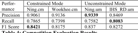
In Table 4, we report the evaluation results based on the test data file test_truth.json con-cealed from development. For constrained mode, we list the top-two results by teams

NCSU_SAS_NING (Ning.cm) and

NCSU_SAS_WOOKHEE (Wookhee.cm). For unconstrained mode, we list the top result by team IHS_RD (IHS_RD.um) and the result by our own unconstrained mode (Ning.um), which was developed after the competition ended.

Perfor-mance

Constrained Mode Unconstrained Mode Ning.cm Wookhee.cm Ning.um IHS_RD.um Precision 0.9061 0.9136 0.9339 0.8469 Recall 0.7865 0.7398 0.7582 0.8083 F1 Score 0.8421 0.8175 0.837 0.8272 Table 4: Competition Evaluation Results

It can be seen that our normalization system has the best F1 score in both constrained mode and unconstrained mode. In fact, our constrained mode has the best F1 score overall, better than our unconstrained mode, which seems counterin-tuitive. Besides, the unconstrained mode is ex-pected to achieve higher recall than the con-strained mode because of its much larger dic-tionary, but the evaluation results show that the unconstrained mode has lower recall and higher precision than the constrained mode. The follow-ing three factors lead to the inferior F1 score and recall by our unconstrained mode:

The much larger canonical form dictionary used by the unconstrained mode contains many rarely used words and having such words as can-didates causes the candidate evaluation compo-nent to be more conservative in selecting candi-dates other than the original tokens (higher preci-sion and lower recall). A potential solution is to use a smaller dictionary of most frequently used words instead of a large dictionary or to use a dictionary with word frequency based on a large corpus.

successfully suggests “Brooklyn” as a candidate for token “Brklyn”, which our constrained mode is incapable of, but the candidate evaluation component fails to select “Brooklyn” as the cor-rect canonical form. A potential solution is to include more context information for candidate evaluation. For example, text likelihood estimat-ed by a CRF model before and after normaliza-tion can be added as classificanormaliza-tion features. Hav-ing word frequency as a feature can also be help-ful.

The binary class labeling in the candidate evaluation component does not differentiate normalization without change (e.g. “car” à “car”) from normalization with change (e.g. “ur” à “your”). As a result, we are unable to tune parameters to favor normalization with change in order to achieve a better trade-off between preci-sion and recall (higher recall and slightly lower precision), which means higher F1 score. A po-tential solution is to change the candidate evalua-tion component into a two-level classificaevalua-tion. The first level classifies whether the normaliza-tion needs any change. If no, then the token itself is output as the normalization result. If yes, then the second level classification assigns a confi-dence score to each candidate that is different from the token and outputs the one with the highest score as the result.

5

Conclusions and Future Work

In this paper, we present a system to perform lexical normalization for English Twitter text, with a constrained mode and an unconstrained mode. Our constrained mode achieves the top F1 score in the W-NUT noisy text normalization competition and outperforms other participants’ unconstrained modes. Our unconstrained mode currently has slightly lower recall and F1 score than the constrained mode, but it has a lot more room for improvement as discussed in the evalu-ation section. Future work includes implement-ing the ideas to improve the unconstrained mode and exploring semi-supervised and unsupervised text normalization. One potential solution for unsupervised text normalization is first clustering tokens based on context (e.g. Brown clustering (Brown et al., 1992)) and then choosing the most frequent token in each cluster as the canonical form for all tokens in that cluster.

Reference

T. Baldwin, M. Catherine, B. Han, Y.B. Kim, A. Rit-ter and W. Xu. 2015. Shared Tasks of the 2015

Workshop on Noisy User-generated Text: Twitter Lexical Normalization and Named Entity Recogni-tion. In Proc. of WNUT.

L. Breiman. 2001. Random Forests. Machine Learn-ing, 45(1), 5-32.

P. Brown, P. deSouza, R. Mercer, V. Della Pietra, J. Lai. 1992. Class-Based n-gram Models of Natural Language. Computational Linguistics, vol. 18, pp. 467–479.

K. Gimpel, N. Schneider, B. O’Connor, D. Das, D. Mills, J. Eisenstein, M. Heilman, D. Yogatama, J. Flanigan, and N. A. Smith. 2011. Part-of-speech tagging for Twitter: Annotation, features, and ex-periments. In Proc. of ACL.

B. Han and T. Baldwin. 2011. “Lexical normalisation of short text messages: Makn sens a #twitter”. In Proc. of ACL.

M. Levandowsky and D. Winter. 1971. Distance be-tween sets. Nature 234 (5): 34–35.

V. Levenshtein. 1966. Binary codes capable of cor-recting deletions, insertions, and reversals. Soviet Physics Doklady 10 (8): 707–710.