Tests for High Dimensional Generalized Linear Models

Munich Personal RePEc Archive

Tests for High Dimensional Generalized

Linear Models

Chen, Song Xi and Guo, Bin

Peking Univeristy and Iowa State University, Peking Univeristy

2014

Online at

https://mpra.ub.uni-muenchen.de/59816/

Tests for High Dimensional Generalized Linear Models

Song Xi Chen and Bin Guo

Peking University and Iowa State University, and Peking University

April 17, 2014

Abstract

We consider testing regression coefficients in high dimensional generalized linear mod-els. By modifying a test statistic proposed by Goeman et al. (2011) for large but fixed dimensional settings, we propose a new test which is applicable for diverging dimension and is robust for a wide range of link functions. The power properties of the tests are evaluated under the setting of the local and fixed alternatives. A test in the presence of nuisance parameters is also proposed. The proposed tests can provide p-values for testing significance of multiple gene-sets, whose usefulness is demonstrated in a case study on an acute lymphoblastic leukemia dataset.

Key words: Generalized Linear Model; Gene-Sets; High Dimensional Covariate; Nuisance

Parameter;U_-statistics.

1

Introduction

linear models under the high dimensional settings has been the focus of latest research. van de Geer (2008) considered variable selection via a LASSO approach. Fan and Song (2010) and Chang et al. (2013) proposed approaches via the sure independence screening of Fan and Lv (2008).

The focus of the paper is on testing for significance of the regression coefficients in high dimensional generalized linear models, which is of important interest to practitioners, for instance in the context of discovering significant gene-sets. The inferential context of gene-set testing encounters both high dimensionality and multiplicity, as genes in different gene-sets can overlap. These two features call for methods which can produce the p-value for the significance of each gene-set, which is an aim of the current paper in the context of the generalized linear models. For fixed dimensional data, the likelihood ratio test and the Wald test have been popular choices as elaborated in McCullagh and Nelder (1989). However, the high dimensionality renders the inapplicability of these tests. There are a set of published works on testing for the coefficients of high dimensional linear regression for the largep(dimension), smalln(sample size) paradigm, which include the tests proposed in Goeman et al. (2006) for an empirical Bayesian formulation, Zhong and Chen (2011) that accommodates the factorial designs, and in Lan et al. (2014) that allows testing on subsets of the regression coefficients. There are also works on the post-variable selection inference associated LASSO and other variable selection methods for the linear models under the sparsity assumption, see Berk et al. (2013), Lee et al. (2014), Taylor et al. (2014), van de Geer et al. (2013) and Zhang and Zhang (2014).

In this paper, we consider testing for high dimensional regression coefficient for the generalized linear models without assuming the non-zero coefficients are sparse. In an important develop-ment, Goeman et al. (2011) proposed a test for the coefficients of high dimensional generalized linear models in the presence of nuisance parameters. The test has provided a much needed tool for performing multivariate tests when the conventional likelihood ratio and the Wald tests are not applicable. While allowing for the dimension p larger than the sample size n, the test of Goeman et al. (2011) was formulated for fixed p.

We propose tests for the entire regression coefficients and part of the regression coefficients in the presence of nuisance parameters for high dimensional generalized linear models with diverging

significant gene-sets in the context of high dimensionality and multiplicity.

The paper is organized as follows. In Section 2, we review the inferential setting for the generalized linear models. Section 3 considers Goeman et al. (2011)’s test for diverging p, which motivates our proposal for the global test in Section 4 and the test with nuisance parameters in Section 5. Results from simulation studies are reported in Section 6. Section 7 presents the case study on the acute lymphoblastic leukemia dataset. All technical details are relegated to the Appendix.

2

Models and existing test

Let Y be a response variable to a p-dimensional covariate X. The generalized linear models (McCullagh and Nelder, 1989) provide a rich collection of specifications for the conditional mean ofY givenX. Although they are intimately connected to the exponential family of distributions, a more general view can be attained via the semiparametric quasi-likelihood of Wedderburn (1974).

Conditioning on the covariate X, there exists a monotone function g(·) and a non-negative function V(·) such that

E(Y|X) =µ(β) = g(XT

β) and Var(Y|X) =V{µ(β);φ}, (2.1)

where β is a p-dimensional regression coefficient, g−1_{(·) is called the link function and φ is a}

dispersion parameter.

Let (X1, Y1), . . . ,(Xn, Yn) be the independent copies of (X, Y). The maximum quasi-likelihood

estimator ˆβn of β can be obtained by solving the quasi-likelihood score equation:

ℓn(β) = n X

i=1

{Yi−g(XT

i β)}g′(XiTβ)Xi

V{µi(β); ˆφ} = 0 (2.2)

where µi(β) = g(XT

i β) and ˆφ is an estimator of φ, which can be obtained via the method

of moment (for instance that given in Chen and Cui, 2003). When the variance function is multiplicative with respect to φ, say V{µ(β);φ}=φV{µ(β)}, there is no need to carry out the initial estimation of φ for the inference on β. The consistency and asymptotic normality of ˆβn

are well established for fixed dimensional covariate (McCullagh and Nelder, 1989). Let β = (β(1)T_{, β}(2)T₎T _{be a partition of the coefficient vector and Xi = (X}(1)T

i , X

(2)T

i )T be the

corresponding partition of the covariates, where β(1) _{and X}(1)

i are p1-dimensional, β(2) and Xi(2)

are p2-dimensional, and p1+p2 =p. Suppose one is interested in testing a hypothesis

H0 :β(2) =β0(2) versus H1 :β(2) 6=β0(2)

on the effect of the covariate X(2)

i while treating β(1) as the nuisance parameter.

When the dimensions p1 and p2 are fixed, modified Wald and the score tests based on the

above hypothesis. However, the high dimensionality often requires that p2 > n, see Pan (2009).

Whenp2 > n, the conventional Wald or the likelihood ratio tests are no longer applicable since the

invertibility of the information matrix is not attainable and the maximum likelihood estimators for the parameters may not be obtained.

Goeman et al. (2011) considered the following test formulation in the case of p2 > n with

g−1_{(·) being the canonical link. To make the discussion more generally applicable, non-canonical}

links are considered via ψ(Xi, β0, φ) =g′(XiTβ0)/V{µi(β0);φ} whereg′ denotes the derivative of

g. The canonical link meansψ(Xi, β0, φ) is a constant. Using the general ψ(·) function does not

alter the formulation of Goeman et al. (2011)’s test. Let ˆβ(1)

0 and ˆφ0 be the estimators of the nuisance parameters β(1) and φ under H0, ˆβ0 =

( ˆβ(1)T

0 , β

(2)T

0 )T, ˆµ0i = µi( ˆβ0), µb0 = (ˆµ01, . . . ,µˆ0n)T and Ψb0 = {ψ(X1,βˆ0,φˆ0), . . . , ψ(Xn,βˆ0,φˆ0)}T.

Moreover, let X(2) _{= (X}(2)

1 , . . . , Xn(2))T, Y = (Y1, . . . , Yn)T and D be the n×n diagonal matrix

that collects the diagonal elements of X(2)_X(2)T_{. The test statistic of Goeman et al. (2011) is}

b

Sn= {(Y−µb0)◦Ψb0}

T_X(2)_X(2)T_{(Y− b

µ0)◦Ψb0}

{(Y_{−bµ0)◦Ψ}b_0}T_D{(Y−µb

0)◦Ψb0}

(2.3)

whereA◦B = (aijbij) for matricesA= (aij) andB = (bij). Note that, under the null hypothesis, the score function of β(2) _is

ℓ2( ˆβ0(1), β

(2)

0 ) =X

(2)T

{(Y_{−bµ0)◦Ψ}b_0}.

Hence, the numerator ofSnb is a quadratic form of the score function, which will be small (large) when the null hypothesis is true (not true). The denominator is a plug-in estimator to the mean of the numerator for standardization.

3

Goeman et al. (2011)’s test when

p

→ ∞

The proposal of Goeman et al. (2011) was formulated for fixed dimensionpwhile allowingp > n. We analyze in this section its properties under the regime of diverging p as n → ∞. It will be shown that the test of Goeman et al. (2011) remains powerful for diverging p when either g or

g′ _{is bounded. At the same time, we reveal a loss of power for the test for some link functions.} The analysis will provide useful insight on how to construct better tests for the case ofp→ ∞.

To make the discussion focused while still being relevant, we concentrate on testing the global hypothesis in the absence of nuisance regression parameters, namely

H0 :β=β0 versus H1 β 6=β0.

To simplify our analysis, we assume E(X) = 0 without loss of generality as otherwiseX can be re-centered by its mean. Throughout the paper, we denote ΣX = cov(X), ǫ =Y −g(X

T_β), ǫ0 =Y −g(XTβ0). We usek · k to denote the Euclidean norm, and for two sequences {an} and

{bn},an≍bn meansan=O(bn) and bn=O(an).

Assumption 3.1. There exists a m-variate random vector Zi = (zi1, . . . , zim)T for some m≥p

so that Xi = ΓZi, where Γ is a p×m constant matrix such that ΓΓT _{= Σ}

X and E(Zi) = 0,

var(Zi) = I_{m, where} I_{m is the m×m identity matrix. Each zij has a finite 8th moment and} E(z4

ij) = 3 + ∆ for a constant ∆>−3, and for any integers ℓν ≥0 and distinct j1, . . . , jq with

Pq

ν=1ℓν ≤8,

E(zℓ1 ij1z

ℓ2 ij2· · ·z

ℓq

ijq) = E(z ℓ1 ij1)E(z

ℓ2

ij2)· · ·E(z ℓq ijq).

Assumption 3.2. Asn → ∞,p→ ∞, tr(Σ2

X)→ ∞and tr(Σ

4

X) = o{tr

2_(Σ2

X)}.

Assumption 3.3. Letfx be the probability density of X and D(fx) be its support. There exist

positive constants K1 and K2 such that E(ǫ2|X = x) > K1 and E(ǫ8|X = x) < K2 for any

x∈D(fx).

Assumption 3.4. gis once continuous differentiable,V(·)>0, and there exist positive constants

c1 and c2 such that c1 ≤ψ2(x, β0, φ)≤c2 for any x∈D(fx).

Assumption 3.1 is used in Bai and Saranadasa (1996) and Zhong and Chen (2011) to facilitate the analysis in ultra high dimensional tests for the means and linear regression. The model contains the Gaussian and some other important multivariate distributions as special cases; see Chen et al. (2009). Assumption 3.2 is a weaker substitute to conditions which are explicit on the relative rates between p and n, for instance, log(p) ≍ n1/3_{, say. It is noted that when all}

the eigenvalues of ΣX are bounded, tr(Σ4X) = o{tr

2_(Σ2

X)} is true for any diverging p, and the

condition allows diverging eigenvalues. Assumption 3.3 and 3.4 are standard in the analysis of generalized linear models, for instance, the assumption G in Fan and Song (2010). Assumption 3.4 is satisfied ifY is from the exponential family with canonical links.

To reduce the amount of notation, we assume the dispersion parameter φ can be ignored in the inference for β. We will consider φ in Section 5 when treating nuisance parameters. To facilitate the analysis, we define three matrices:

∆β,β0 =E[{g(X T

β)−g(XT

β0)}ψ(X, β0)X],

Σβ(β0) =E[V{g(XTβ)}ψ2(X, β0)XXT] and

Ξβ,β0 =E[{g(X T

β)−g(XT

β0)}2ψ2(X, β0)XXT].

The test statistic Snb of Goeman et al. (2011) can be expressed as

b

Sn= 1 +Un/An where

Un =

1

n n X

i6=j

{(Yi−µ0i)(Yj −µ0j)ψ(Xi, β0)ψ(Xj, β0)XiTXj} and

An= 1

n n X

i=1

In additional to the remark made at end of the last section regarding the meaning of the statistic

b

Sn, more insight can be made via the means of Un and An. Derivations show that the means are, respectively,

µUn = (n−1)∆

T

β,β0∆β,β0 and µAn = tr{Σβ(β0) + Ξβ,β0}. (3.1)

We note that for the generalized linear models, the difference between β and β0 is measured by

g(XT_β)−g(XT_β

0), which is reflected by ∆β,β0 and Ξβ,β0 defined above. Hence,Un measures the

differenceg(XT_β)−g(XT_β

0), and An is a certain measure of the noise.

Lemma A.1 in the Appendix shows that the variances of Un and An are respectively

σ2An =n

−1_E{ǫ4

0ψ4(X, β0)(XTX)2} −E2{ǫ20ψ2(X, β0)(XTX)}

and

σU2n = 4(n−2)(1−n

−1_)ξ

1+ 2(1−n−1)ξ2 (3.2)

whereξ1 = ∆Tβ,β0{Σβ(β0)+Ξβ,β0}∆β,β0−(∆ T

β,β0∆β,β0)

2_{and ξ}

2 = tr{Σβ(β0)+Ξβ,β0}

2_−(∆T

β,β0∆β,β0)

2_.

From the central limit theorem, even p→ ∞,

σ−1

An(An−µAn) d

→N(0,1) as n → ∞.

By Taylor expansion,

b

Sn= 1 +µ−An1µUn−µ

−2

AnµUn(An−µAn) +µ

−1

An(Un−µUn) +µ

−3

AnµUn(An−µAn)

2_{+· · · . (3.3)}

To identify the leading order term of (3.3), we consider two families of alternative hypothesis which produce different leading order terms. One is the so-called “local” alternatives:

L_{β =}

β0 ∈Rp

∆Tβ,β0ΣX∆β,β0 =o{n

−1_tr(Σ2

X)} and either {g(X

T_β)−g(XT_β

0)}2 =O(1) a.s.

or (β−β0)TΣX(β−β0) =O(1) and |g′(t)| ≤C0 for any t∈(−∞,∞)

;

(3.4)

for a positive constant C0. The other is the so-called “fixed” alternatives:

LF

β =

β0 ∈Rp

∆Tβ,β0Ξβ,β0∆β,β0 =o{n

−1_tr(Ξ2

β,β0)} and tr(Σ

2

X) = o{tr(Ξ

2

β,β0)}

. (3.5)

Clearly, the H0 is embedded in the “local” alternatives Lβ. While Lβ encompasses β where

the difference k∆β,β0k is relatively small, it also includes β0 not necessarily close to the true β

when either g is uniformly bounded as in the logistic and the probit models, or g′ _{is bounded} as in the linear regression. We use the term “local” simply because H0 is part of Lβ. It is

noticed thatLF

β is applicable to models with unboundedg′ function such as Poisson or Negative

Binomial regression.

If β0 ∈Lβ, the proof of Theorem 1 shows that

σ2An =O(n

−1_µ2

An) and σ

2

Un = 2tr{Σβ(β0) + Ξβ,β0}

which imply that

b

Sn= 1 +µ−1

AnµUn+µ

−1

An(Un−µUn) +op(µ

−1

AnσUn). (3.7)

The above analysis shows that under the “local” alternatives, the test statisticSnb is dominated by a linear function of Un. It can be shown that this is the same as the fixed dimensional case, the setting of Goeman et al (2011)’s proposal. This is due to the fact that the quadratic term and beyond in the Taylor expansion (3.3) can be controlled in the case of diverging pif either g

or its derivative is bounded underL_β.

Let σ2

b

Sn = 2tr{Σβ(β0) + Ξβ,β0}

2_tr−2_{Σ

β(β0) + Ξβ,β0}, which is the leading order variance of b

Sn under L_β.

Theorem 1. Suppose Assumptions 3.1-3.4 hold, then under the “local” alternatives L_β,

σ_S−_b1

n(

b

Sn−1−µ−An1µUn) d

→N(0,1) as n → ∞ and p→ ∞.

Under the null hypothesis,µ−1

AnµUn = 0 andσ

2

b

Sn = 2tr{Σ

2

β0(β0)}tr

−2_{Σ

β0(β0)}. To formulate a

test procedure based on the asymptotic normality, we need to estimateσSbnand hence tr{Σ

2

β0(β0)}

and tr2_{Σ

β0(β0)}. Let

\

tr{Σ2

β0(β0)}=

1

n(n−1)

n X

i6=j

{Yi−g(XT

i β0)}2{Yj −g(XjTβ0)}2ψ2(Xi, β0)ψ2(Xj, β0)(XiTXj)2

and

\

tr2_{Σ

β0(β0)}=

1

n(n−1)

n X

i6=j

{Yi−g(XiTβ0)}2{Yj −g(XjTβ0)}2ψ2(Xi, β0)ψ2(Xj, β0)(XiTXi)(XjTXj)

.

(3.8) Lemma A.3 in the Appendix shows that both are ratioly consistent such that under H0

\

tr{Σ2

β0(β0)}

tr{Σ2

β0(β0)} p

→1 and

\

tr2_{Σ

β0(β0)}

tr2_{Σ

β0(β0)} p

→1 as n→ ∞.

Theorem 1 and the Slutsky Lemma lead to an asymptotic α-level test that rejects H0 if

b

Sn >1 +zα2tr{Σ\2

β0(β0)}/

\

tr2_{Σ

β0(β0)} 1/2

, (3.9)

where zα is the upper α-quantile of N(0,1).

Goeman et al. (2011) approximated the null distribution of Snb by a ratio of quadratic forms based on normally distributed variables, which involves a numerical inversion of the characteristic function. A R package “globaltest” is available at www.bioconductor.org to implement the algorithm. The critical value obtained via the procedure of Goeman et al. (2011) is asymptotically equivalent to the right hand side of (3.9) under H0 in the case of p → ∞, which is confirmed

by our simulation study. We will use the explicit critical value in (3.9) in the following power analysis.

Define the power of the test in (3.9) under the “local” alternatives L_{β as}

Ω(β, β0) = P

b

Sn>1 +zα2tr{Σ\2

β0(β0)}/

\

tr2_{Σ

β0(β0)} 1/2

β0 ∈Lβ

Corollary 1. Under Assumptions 3.1-3.4 and the “local” alternatives L_β,

Ω(β, β0) = Φ −zα+

nk∆β,β0k

2

2tr{Σβ(β0) + Ξβ,β0}2 1/2

!

{1 +o(1)} as n→ ∞ and p→ ∞.

The corollary shows that the power of the test in (3.9) is determined by

SNR(β, β0) =

nk∆β,β0k

2

2tr{Σβ(β0) + Ξβ,β0}2 1/2.

We note thatk∆β,β0k

2 _=kE[{g(XT_β)−g(XT_β

0)}ψ(X, β0)X]k2 measures the difference between

H0 andH1, and can be viewed as the signal of the test problem. At the same time,

2tr{Σβ(β0)+

Ξβ,β0}

21/2 _{can be regarded as the noise due to its close connection to the standard deviation of}

b

Sn. Hence SNR(β, β0) is the signal-to-noise ratio of the test.

Let λ1 ≤ · · · ≤ λp be the eigenvalues of ΣX and λm0 be the smallest non-zero one for a

m0 ∈ {1, . . . , p}. Since ∆Tβ,β0ΣX∆β,β0 ≤ λpk∆β,β0k

2 _{and tr(Σ}2

X) ≥ λ

2

m0(p −m0), a sufficient

condition that ensures the first component of L_{β is}

k∆β,β0k

2 _=o{λ−1

p λ2m0n

−1_(p−m

0)}. (3.10)

Now let ˜λ1 ≤λ˜2 ≤ · · · ≤λp˜ be the eigenvalues of Σβ(β0) + Ξβ,β0. Assumption 3.3 and Lβ imply

that each ˜λi is bounded below and above by constant multiple of λi. Using the same argument leading to (3.10), we can show that SNR(β, β0) is bounded within

nk∆β,β0k

2_{2˜λ2

p(p−m0)}−1/2, nk∆β,β0k

2_{2˜λ2

m0(p−m0)}

−1/2_.

Thus, if k∆β,β0k is a larger order than n

−1/2_λ1/2

p (p−m0)1/4, SNR(β, β0) → +∞ and hence the

power converges to 1. If k∆β,β0k is a smaller order (weaker) than n

−1/2_λ1/2

m0(p−m0)1/4, the

test does not have power beyond the significant level α. Non-trivial power Ω(β, β0) is attained

if k∆β,β0k ≍n

−1/2_λ1/2

p (p−m0)1/4.

Let us evaluate the power of the test under the “fixed” alternativesLF

β , which is denoted as

ΩF(β, β0) = P

b

Sn >1 +zα2tr{Σ\2

β0(β0)}/

\

tr2_{Σ

β0(β0)} 1/2

β0 ∈LβF

.

Unlike the “local” alternatives case, the leading order terms under the “fixed” alternatives involve an additional termµ−2

AnµUn(An−µAn), as shown in the proof of Theorem 2. This term is a

smaller order term in the fixed dimensional case as considered in Goeman et al. (2011). It is also ignorable in the high dimensional case when eithergorg′_{are bounded, as have been shown earlier.} However, it may not be the case under the “fixed” alternatives. Having µ−2

AnµUn(An−µAn) does

not generate more signal for the test, but can increase the variance and hence causes a reduction in the power.

To make this point explicit, we consider a specific case of the “fixed” alternatives where

k∆β,β0k

2 _≍nδ−1_tr1/2_(Ξ2

β,β0) and

E[{g(XT_β)−g(XT_β

0)}4ψ4(X, β0)(XTX)2]

E2_[{g(XT_β)−g(XT_β

0)}2ψ2(X, β0)(XTX)]

≍n1−2δ (3.11)

Assumption 3.5. Asn → ∞,p→ ∞, tr(Ξ2

β,β0)→ ∞ and tr(Ξ

4

β,β0) =o{tr

2_(Ξ2

β,β0)}.

Theorem 2. Under Assumptions 3.1-3.5, (3.11) and the “fixed” alternatives LF

β,

ΩF(β, β0) = Φ

1 (1 +τ2₎1/2

−zα+ nk∆β,β0k

2

{2tr(Ξ2

β,β0)}

1/2

!

{1 +o(1)} (3.12)

as n → ∞, p→ ∞, where τ2 _{= (µ}2

Unσ

2

An)/(µ

2

Anσ

2

Un)∈(0,∞) is a constant.

The reason for obtaining the power expression in (3.12) is that under the conditions of The-orem 2,σ2

An =O(n

−2δ_µ2

An), σ

2

Un = 2tr(Ξ

2

β,β0){1 +o(1)}and b

Sn= 1 +µ−1

AnµUn −µ

−2

AnµUn(An−µAn) +µ

−1

An(Un−µUn) +op(µ

−1

AnσUn). (3.13)

Note that, both µ−2

AnµUn(An−µAn) and µ

−1

An(Un−µUn) are the joint leading order terms of Snb .

The role of condition (3.11) is to make the quadratic terms and beyond in the Taylor expansion (3.3) ofSnb are of smaller orders of the two linear terms in (3.13). A consequence of theAn−µAn

term in the leading order term leads to τ2 _{appeared in the power function, which causes a power}

reduction as reflected by the first fraction inside Φ in (3.12).

If the second part of (3.11) is more relaxed so that it is of a larger order ofn1−2δ _{but a smaller}

order of n1−δ_{, the power expression (3.12) still holds but with τ}2 _{→ ∞. This means a dramatic}

deterioration in the power. If the order of the second term in (3.11) is higher than n1−δ_{, the}

quadratic terms and beyond in the expansion (3.3) will be of larger orders than the linear terms in (3.13), making the power analysis much harder to accomplish and the power performance unpredictable since the main signal bearing term Un−µUn is no longer important.

4

A new proposal

An important insight acquired in the previous section is that the An term in the statistic

b

Sn = 1 +Un/An

does not contribute to the signal of the test but can increase the variance (noise) and hence can adversely affect the power. Although An has a negligible effect on the power under the “local” alternatives L_{β, its role on the power becomes more pronounced under the “fixed” alternatives}

LF

β . Dividing byAnis a standard formulation that dates back to the Fisher’s F-test for regression

coefficients. However, under the high dimensionality, doing so may not be necessary since its contribution to the variance (noise) can be significant as shown in Theorem 2.

The above consideration leads us to propose a statistic by excludingAn fromSnb . Specifically, we consider using

Un =

1

n n X

i6=j

as the test statistic. Comparing with the involved expansion (3.3) ofSnb ,Un has a much simpler form. Despite being simpler, it captures the signal of the test since E(Un) = (n−1)k∆β,β0k

2 _as

shown in (3.1). We will demonstrate in this section that a test based on Un can achieve better power for diverging p than Goeman et al. (2011)’s test under LF

β while maintaining the same

asymptotic power under L_β.

We still consider testing the global hypothesis H0 : β = β0 in this section. A test for the

presence of the nuisance parameters will be unveiled in the next section. Recall from (3.6) that under L_β,σ2

Un = 2tr{Σβ(β0) + Ξβ,β0}

2_{{1 +o(1)}.}

Theorem 3. Under Assumptions 3.1-3.4 and the “local” alternatives L_β,

Un−nk∆β,β0k

2

2tr{Σβ(β0) + Ξβ,β0}2 1/2

d

→N(0,1) as n → ∞ and p→ ∞.

Theorem 3 implies that under the null hypothesis,

Un

2tr{Σ2

β0(β0)} 1/2

d

→N(0,1) as n → ∞and p→ ∞.

Using tr{Σ\2

β0(β0)} given in (3.8) to estimate tr{Σ

2

β0(β0)}, the proposed α-level test rejects H0 if Un> zα2tr{Σ\2

β0(β0)} 1/2

. (4.1)

LetΩ(e β, β0) = P

Un> zα2tr{Σ\2

β0(β0)} 1/2

β0 ∈Lβ

be the power of the above test under the “local” alternatives L_β.

Corollary 2. Under Assumptions 3.1-3.4 and the “local” alternatives L_β,

e

Ω(β, β0) = Φ −zα+

nk∆β,β0k

2

2tr{Σβ(β0) + Ξβ,β0}2 1/2

!

{1 +o(1)} as n→ ∞ and p→ ∞.

We note here that the power of the proposed test is asymptotically equivalent to Ω(β, β0)

of Goeman et al. (2011) given in Corollary 1. This is expected since in the case of the “local” alternatives L_β,

1 +µ−An1µUn+µ

−1

An(Un−µUn) (4.2)

is the leading order term of Sbn. Hence, the two tests are asymptotically equivalent.

From the proof of Theorem 4, the asymptotic variance of Un under the “fixed” alternatives

LF

β is

σU2n = 2tr(Ξ

2

β,β0){1 +o(1)}.

LetΩeF_{(β, β} 0) = P

Un> zα2tr{Σ\2

β0(β0)} 1/2

β0 ∈LβF

be the power under LF

β .

Theorem 4. Under Assumptions 3.1-3.5 and the “fixed” alternatives LF

β ,

e

ΩF(β, β0) = Φ −zα+

nk∆β,β0k

2

{2tr(Ξ2

β,β0)}

1/2

!

The conditions in Theorem 4 are much simpler than those in Theorem 2, as condition (3.11) is not needed. To compare the two power functions under the “fixed” alternatives while assuming the conditions of Theorem 2, (3.11) implies that

nk∆β,β0k

2

{2tr(Ξ2

β,β0)}

1/2 ≍n

δ_{→ ∞.}

A power gain is evident asΩeF_{(β, β}

0)>ΩF(β, β0) asymptotically, since the power function (3.12)

has an extra τ2 _{in the denominator.}

5

Test with nuisance parameter

We consider testing for parts of the regression coefficient vectorβ. This is motivated by practical needs to consider the significance for a subset of covariatesX(2)_{, in the presence of other covariates} X(1)_{. For instance, one may have both gene expression levels and demographic variables collected}

in a study on the cause of a disease. The researcher may be interested only in the genetic effect. In this case, the demographic coefficients together with the dispersion parameter may be viewed as nuisance parameters.

Without loss of generality, we partitionβ = (β(1)T_{, β}(2)T₎T _{and denote the nuisance parameters} θ = (β(1)T_{, φ)}T_{, where φ is the nuisance dispersion parameter. Suppose the dimension of θ is p}

1

and that of β(2) _isp

2. It is of interest to test

H01:β(2) =β0(2) versus H11 :β(2) 6=β0(2).

A test statistic along the line of the global test statistic Un will be proposed. To this end, the nuisance parameters β(1) _{and φ have to be estimated first under H}

01. The quasi-likelihood

score of β(1) _is

ℓ1(β(1), β(2), φ) = X(1)T{(Y−µ)◦Ψ},

where X(1) _{is similarly defined as X}(2) _{in Section 2, Ψ = {ψ(X}

1, β, φ), . . . , ψ(Xn, β, φ)}T and

µ={µ1(β), . . . , µn(β)}T. The maximum quasi-likelihood estimator of β(1) underH01 solves

ℓ1(β(1), β0(2),φˆ0) = 0,

which is denoted as ˆβ(1)

0 , by plugging-in ˆφ0, either a maximum likelihood estimator or a moment

estimator of φ as elaborated in McCullagh and Nelder (1989) and Chen and Cui (2003). Let ˆ

β0 = ( ˆβ0(1)T, β

(2)T

0 )T, ˆθ0 = ( ˆβ0(1)T,φˆ0)T and ˆµ0i =µi( ˆβ0).

We consider a statistic,

e Un= 1

n n X

i6=j

{(Yi−µˆ0i)(Yj −µˆ0j)ψ(Xi,βˆ0,φˆ0)ψ(Xj,βˆ0,φˆ0)Xi(2)TX (2)

j }. (5.1)

Let ΣX(i) =E(X

Assumption 5.1. Asn → ∞,p2 → ∞, tr(Σ2_X(2))→ ∞and tr(Σ_X(2)4 ) = O{n−1tr2(Σ2_X(2))}.

Assumption 5.2. As n→ ∞,p1n−1/4 →0 and there exists aθ∗ = (β∗(1)T, φ∗)T∈Rp1 such that

kθˆ0−θ∗k =Op(p1n−1/2), and in particular under H01, θ∗ = θ, where θ = (β(1)T, φ)T is the true

value of nuisance parameter.

Assumption 5.3. There exists a positive constant λ0 such that 0 < λ0 ≤ λmin(ΣX(1)) ≤

λmax(ΣX(1)) ≤ λ

−1

0 < ∞, where λmin(ΣX(1)) and λmax(ΣX(1)) represent the smallest and largest

eigenvalues of the matrix ΣX(1) respectively.

Assumption 5.4. There exist positive constants c1 and c2 such that for β0∗ = (β∗(1)T, β

(2)T

0 )T

whereβ∗(1) _{is defined in Assumption 5.2,c}

1 ≤ψ2(x, β0∗, φ∗)≤c2 and [∂ψ{g(t)}/∂g(t)]2 |t=xT_β∗

0 ≤

c2 for any x∈D(fx) and a neighborhood ofxTβ0∗.

These assumptions are variations of Assumptions 3.2-3.4 in Section 2. Specifically, Assump-tion 5.1 is equivalent to AssumpAssump-tion 3.2 in the presence of the nuisance parameter. The re-quirement of the growing rate ofp1 being slower thann1/4 is to allow accurate estimation of the

nuisance parameter under the high dimensionality. Assumption 5.2 maintains that the initial estimator ˆθ0 is consistent to a θ∗ which may deviate from the true parameter θ, when the

dis-crepancy between β(2)

0 and β(2) is large. The θ∗ is the one that minimizes the Kullback-Leibler

divergence between the misspecified model underH01 and the model underH11; see van de Vaart

(2000) for details. Assumption 5.3 is easier to be satisfied due to ΣX(1)’s dimension is much more

manageable than the case considered in the previous section. Assumption 5.4 is an updated version of Assumption 3.4 to suit the case of nuisance parameters.

To analyze the power, we introduce two matrices

∆(2) β,β∗

0 =E[{g(X

T_β)−g(XT_β∗

0)}ψ(X, β0∗, φ∗)X(2)] and

Σ(2) β (β

∗

0) = E[V{g(X

T

β)}ψ2(X, β₀∗, φ∗)X(2) X(2)T

],

which are counterparts of ∆β,β0 and Σβ(β0) used in the study of the global test. There is no need

to define a counterpart of Ξβ,β0 since the second part of the “local” alternatives Lβ(2) defined

below makes it unnecessary.

The involvement of the estimated nuisance parameter ˆθ0 does complicate the power

analy-sis. To expedite the study, our analysis is confined under the following family of the “local” alternatives

L β(2) =

β(2)

0 ∈Rp2

∆(2)Tβ,β∗

0ΣX(2)∆ (2) β,β∗

0 =o{n

−1_tr(Σ2

X(2))} and E{g(X T

β)−g(XT

β₀∗)}4 =o(n−3/2)

.

We note here that the second component of L

β(2) is stronger than that in L_β in (3.4), which

simplifies the analysis in the presence of the nuisance parameter.

Theorem 5. Under Assumptions 3.1, 3.3, 5.1-5.4, and the “local” alternatives L

β(2), e

Un−nk∆β,β∗

0k

2

2tr{Σ(2) β (β0∗)}2

1/2

d

To formulate a test procedure, we use

b

Rn= 1

n(n−1)

n X

i6=j

(Yi−µˆ0i)2(Yj−µˆ0j)2ψ2(Xi,βˆ0,φˆ0)ψ2(Xj,βˆ0,φˆ0)(Xi(2)TX (2) j )2

to estimate tr{Σ(2)

β (β0∗)}2 under H01. Lemma A.6 in the Appendix shows that the estimator is

ratioly consistent underH01, that is

b Rn

tr{Σ(2) β (β0∗)}2

p

→1 as n → ∞.

Hence, an asymptotic α-level test rejects H01 if Une > zα(2Rnb )1/2 and the proofs of Theorem

5 and Lemma A.6 show that the test procedure is invariant to the scale transformation of Y. Define the power of the test under the “local” alternatives L

β(2)

e

Ω(2)_{(β, β}∗

0) = P

e

Un> zα(2Rnb )1/2 |β(2)

0 ∈Lβ(2)

.

Corollary 3. Under Assumptions 3.1, 3.3, 5.1-5.4 and the “local” alternatives L

β(2),

e

Ω(2)

(β, β∗

0) = Φ −zα+

nk∆(2) β,β∗

0k

2

2tr{Σ(2) β (β∗)}2

1/2

!

{1 +o(1)} as n → ∞ and p2 → ∞.

The power Ωe(2)_{(β, β}∗

0) has a similar form as Ω(e β, β0) in Corollary 2. This is expected due to

the close connection between the two tests and their test statistics respectively. We note that the denominator inside Φ only involves Σ(2)

β (β∗) due to the second part of Lβ(2).

We did not study the power under the “fixed” alternatives similar to the one in Section 3, as we would expect the power performance would be largely similar to the one depicted in Section 4. We also did not study the power property of the Goeman et al. (2011)’s test with nuisance parameter as the analysis would be quite involved due to the division of An term and the estimated nuisance parameter. However, we would expect similar power properties revealed in the previous section would prevail, namely the power of Goeman et al. (2011)’s test would be hampered when g′ _{is unbounded. This is indeed confirmed by the simulation results reported in} the next section.

6

Simulation studies

(3.9) based on the asymptotic normality. Both had close size, confirming the fact that the two forms of the critical value lead to equivalent tests.

Throughout this section, the covariates Xi = (Xi1, . . . , Xip)T were generated according to a

moving average model

Xij =ρ1Zij+ρ2Zi(j+1)+· · ·+ρTZi(j+T−1), j = 1, . . . , p;

for some T < p, whereZi = (Zi1, . . . , Zi(p+T−1))T were from a (p+T −1) dimensional standard

normal distribution N(0,I_{p+T−1). The coefficients {ρl}}T

l=1 were generated independently from

theU(0,1) distribution, and were treated as fixed once generated. Here,T was used to prescribe different levels of dependence among the components of the high dimensional vectorXi. We had experimented T = 5,10 and 20, and only reported the results for T = 5 since those for T = 10 and 20 were largely similar.

Four generalized linear models were considered in the simulation study: the logistic, linear, Poisson and Negative Binomial regression models. In the logistic regression model, the condi-tional mean of the response Y was given by

E(Yi|Xi) =g(XT i β) =

exp(XT i β)

1 + exp(XT iβ)

,

and conditioning on Xi, Yi ∼Bernoulli{1, g(XT

i β)}. In the linear regression, E(Yi|Xi) = g(XT

i β) =X

T i β,

and conditioning on Xi, Yi ∼ N(XT

i β,1). We note here that the test is invariant with respect

to the nuisance dispersion parameter σ2_{. Hence, setting σ = 1 was not crucial for the test}

performance. In the Poisson regression,

E(Yi|Xi) =g(XT

i β) = exp(XiTβ),

and conditioning onXi,Yi ∼Poisson{g(XT

iβ)}. The setup for the Negative Binomial model was Y|λ∼Poisson(λ) and λ∼Gamma{exp(XT

β),1}.

The conditional distribution ofY givenXis the negative binomial distributionN B{exp(XT_β),1/2},

which prescribes an over-dispersion to the Poisson model, and makes it a popular alternative to the Poisson regression in practice.

To create regimes of high dimensionality, we chose a relationshipp= exp(n0.4_{) and specifically}

considered (n, p) = (80,320) and (200,4127) in the simulations. Seven nominal type I errors ranging from 0.05 to 0.2 were considered, and the corresponding empirical sizes and powers were evaluated from 2000 replications.

We first considered testing the global hypothesis

In designing the alternative hypothesis, for the linear model we made kβk2 _{= 0.2 and chose the}

first five coefficients inβ to be non-zero of equal magnitude and the rest of the coefficients to be zero. For the other three models,kβk2 _{= 2. Hence, the non-zero coefficients were quite sparse.}

In order to have a reasonable range for the response variable, as in Goeman et al. (2011), we restricted E(Yi|Xi) between exp(−4)/{1 + exp(−4)}= 0.02 and exp(4)/{1 + exp(4)}= 0.98 for the logistic model, between −1000 and 1000 for the linear model, and between exp(0) = 1 and exp(4) = 55 for the Poisson and Negative Binomial models respectively.

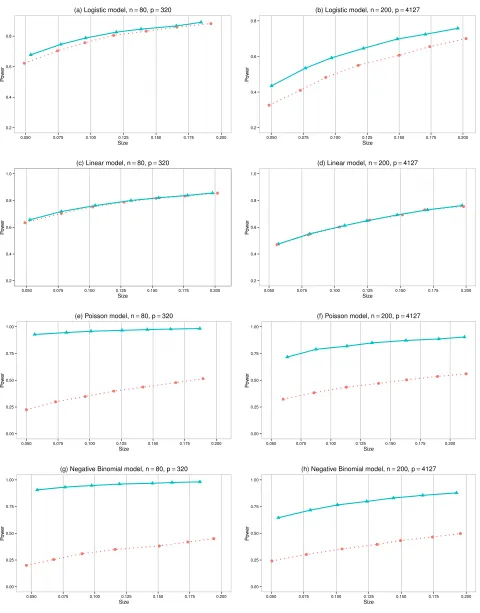
The empirical power profiles (curves of empirical power versus empirical size) of the global tests were plotted in Figure 1. It is observed that the proposed global test and Goeman et al. (2011)’s test had largely similar power profiles for the logistic and linear models as displayed by Panels (a) - (d) of the figure. This is consistent with our findings in Corollaries 1 and 2, which indicate that both tests have the same asymptotic powers under the “local” alternatives L_β.

Panels (a) and (b) of Figure 1 displayed that the proposed test had a slightly higher power than Goeman et al. (2011)’s test in the case of the logistic model. This can be understood as the impact ofAn term on the variance of Snb despite its being the second order under the “local” alternatives.

Panels (c)-(d) of Figure 1 displayed that both Goeman et al. (2011)’s test and the proposed test had almost identical size and power performance in the linear regression model. This confirms the provision of our theory regarding boundedg′ _{as shown in Corollary 1.}

Panels (e)-(h) showed a much larger discrepancy in the power profiles between the two tests for the Poisson and Negative Binomial models with the proposed test being significantly more powerful. It is noted that both models have unbounded g′_{, which imply that the testing was} operated in the regime of the “fixed” alternatives LF

β. The simulated power profiles confirmed

the findings in Theorem 2 in that an unbounded g′ _{function can adversely impact the power of} Goeman et al. (2011)’s test, whereas the proposed test withstands such situations due to its test statistic formulation.

We then conducted simulation for testing

H0 :β(2) = 0p2×1 versus H1 :β (2) _{6= 0}

p2×1 (6.2)

in the presence of nuisance parameterβ(1) _{for the same four generalized linear models considered}

above. The nuisance parameter β(1) _{was p}

1 = 10 dimensional, generated randomly from U(0,1)

as in the design of the global hypothesis. We still chose (n, p2) = (80,320) and (200,4127) by

assigning p2 = exp(n0.4). To evaluate the power of the test, the first five elements of β(2) were

set to be non-zero of equal magnitude withkβ(2)_k2 _{= 0.5 for the linear model and kβ}(2)_k2 _{= 2 for}

the other three generalized linear models, while the rest of β(2) _{were zeros.}

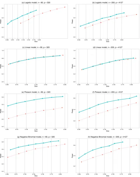
The power profiles of the proposed and Goeman et al. (2011)’s tests were displayed in Figure 2. It is observed from Panel (a) of Figure 2 that, for the logistic model with n = 80 and

p2 = 320, the test of Goeman et al. (2011) had very severe size distortion, which may be due to

presence for the test of Goeman et al. (2011) was largely absent for the proposed test. Figure 2 shows that the proposed test had quite reasonable power with good control of the type I error. For the Poisson and Negative Binomial models (Panels (e)-(h)), we observed that the proposed test had much more advantageous power profiles than those of Goeman et al. (2011)’s test. The latter was similar to the global tests demonstrated in Figure 1.

7

Case study

We analyze a dataset that contains microarray readings for 128 persons who suffer the acute lymphoblastic leukemia (ALL). The dataset also has information on patients’ age, gender and response to multidrug resistance. Among the 128 individuals, 75 of them were patients of the B-cell type leukemia which were classified further to two types: the BCR/ABL fusion (35patients) and cytogenetically normal NEG (40 patients). The dataset has been analyzed by Chiaretti et al. (2004), Dudoit et al. (2008), Chen and Qin (2010) and Li and Chen (2012) and others motivated from different aspects of the inference.

Biological studies have shown that each gene tends to work with other genes to perform certain biological missions. Biologists have defined gene-sets under the Gene Ontology system which provides structured vocabularies producing names of Gene Ontology terms. The gene-sets under the Gene Ontology system have been classified to three broad functional categories: Biological Processes, Cellular Components and Molecular Functions. There have been a set of research works focusing on identifying differentially expressed sets of genes in the analysis of gene expression data; see Efron and Tibshirani (2007), Rahmatallah et al. (2012). After preliminary gene-filtering with the algorithm proposed in Gentleman et al. (2005), there were 2250 unique Gene Ontology terms in Biological Processes, 328 in Cellular Component and 402 in Molecular Function categories respectively, which involved 3265 genes in total.

Our aim here is to identify gene-sets within each functional category, which are significant in determining the two types of B-cell ALL: BCR/ABL fusion or cytogenetically normal NEG. We formulate it as a binary regression with the response Yi being 1 if the ith patient had the BCR/ABL type ALL and 0 if had the NEG type. The covariate of theith patient corresponding to a gene-set, label byg in the subscript, isXig = (X(1)T

ig , X

(2)T

ig )T, whereX (1)

ig contains the gender,

age and the patient’s response to multidrug resistance (1 if negative and 0 positive), and X(2)

ig is

the vector of gene expression levels of thegth Gene Ontology term.

We considered the logistic and probit models for the gene-set data due to the binary nature of the response variable. The two models are, respectively,

E(Yi|X(1) ig , X

(2) ig ) =

exp(X(1)T

ig βg(1)+X (2)T ig βg(2))

1 + exp(X(1)T

ig β

(1)

g +X_ig(2)Tβg(2))

and

E(Yi|X(1) ig , X

(2)

ig ) = Φ(X (1)T

ig β

(1)

g +X

(2)T

ig β

(2) g ).

For the leukemia data, it is of fundamental interest in discovering significant Gene Ontology terms while considering the effects of the three covariates in X(1)_{, namely by treating β}(1)

nuisance parameter and testing the following hypothesis:

H0 : βg(2) = 0 versus H1 : βg(2) 6= 0.

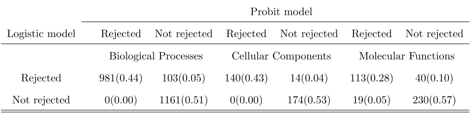
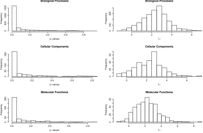
By controlling the false discovery rate (Benjamini and Hochberg, 1995) at 0.01, 1084 gene-sets in Biological Processes, 154 in Cellular Components and 153 in Molecular Function were found significant under the logistic model, and 981 in Biological Processes, 140 in Cellular Components and 132 in Molecular Function were significant under the probit model. Table 1 reports the two by two rejection/non-rejection classification between the tests under the two models. It shows that the testing results were largely agreeable between the two models. This was especially the case for the gene-set categories of Biological Processes and Cellular Components, with more than 90% of the gene-sets rejected under the logistic model being also rejected under the probit model, and the non-rejected gene-sets matched perfectly. The discrepancy in the test conclusions got larger for gene-sets in the Molecular Function category. But still, the percentages of agreement between the two models exceeded 72% in the rejection and 92% in the non-rejection. These showed again the testings under the two models attained similar results.

We also carried out the global test for the significance of the entire regression coefficient vectorβg by performing test on

H0 : βg = 0 versus H1 : βg 6= 0

where βg = (β(1)T

g , βg(2)T)T with the first three coefficients corresponding to the three non-genetic

covariates: the gender, age and multidrug resistance. We note that the value of the standardized global test statistics under the logistic and the probit models were identical. This is because under the H0, g(XiTβg) = g(0) = 0.5 and ψ(Xi,0) are constant for both models, which means

that ψ(Xi,0) are canceled out in the standardized test statistics. Hence, the test procedures were identical for testing the global hypothesis regarding each gene-set under both the logistic and probit models.

8

Discussion

As the generalized linear models are widely used tools in analyzing genetic data, the proposed tests, being more adaptive to the high dimensionality, are useful additions to the existing test procedures for the significance of regression coefficients. As shown in the case study, testing for the significance of gene-sets requires high dimensional multivariate test procedures which can produce p-values under both high dimensionality and multiplicity (as genes in gene-sets can overlap). The proposed tests and the tests of Goeman et al. (2011) are such tests which can be used for the gene-sets testing in conjunction with the FDR procedure when testing a large number of hypotheses simultaneously.

The test of Goeman et al. (2011) was proposed for fixed dimensional p. We have found it is quite resilient to the diverging p in both theoretical and empirical analysis, as long as either the inverse of the link function or its derivative is bounded. The latter encompasses the logistic and linear regression models. The proposed tests are designed to improve the performance of Goeman et al. (2011)’s test for diverging p. This is especially the case when the first order derivative of the inverse of the link function is unbounded, when the high dimensionality can insert adverse influence on the test of Goeman et al. (2011). The proposed test statistics due to their simpler formulations can avoid some of the high dimensional effects, and hence lead to better performances in terms of more accurate size approximation and more power. Of course, when p is of fixed dimension, the test of Goeman et al. (2011) may be used and the proposed test may not be valid.

There have been works on the post-variable selection inference associated LASSO and other variable selection methods for the linear models as in Berk et al. (2013) , Lee et al. (2014), Taylor et al. (2014), van de Geer et al. (2013) and Zhang and Zhang (2014). These methods are based on the sparsity assumption that the non-zero regression coefficients are sparsely populated. The sparsity assumption is quite hard to be validated from data. Our proposed tests are valid without the sparsity assumption and may be used first when the sparsity level of a testing problem is unknown. More research is needed on how to combine the two strains of inference methods together in the setting of high dimensional generalized linear models.

Appendix

In this section, we provide technical proofs to the main results reported in Section 3-5. To establish the results of the paper, we introduce three lemmas whose proofs are available in Chen and Guo (2014).

We define a few notations:

ǫi =Yi−g(XT

Lemma A.1. The expectations and variances of An and Un are respectively

µAn = tr{Σβ(β0) + Ξβ,β0}, µUn = (n−1)∆

T

β,β0∆β,β0, σA2n =n

−1_Eǫ4 0ψ04(X

T

X)2 −E2ǫ2₀ψ₀2(XT

X) and

σ_U2_n = 4(n−2)(1−n−1_)ξ

1+ 2(1−n−1)ξ2

whereξ1 = ∆Tβ,β0{Σβ(β0)+Ξβ,β0}∆β,β0−(∆ T

β,β0∆β,β0)

2 _{and ξ}

2 = tr{Σβ(β0)+Ξβ,β0}

2_−(∆T

β,β0∆β,β0)

2_.

Lemma A.2. Under Assumptions 3.1-3.4 and the “local” alternatives L_β,

σ2_Un = 2tr{Σβ(β0) + Ξβ,β0}

2_{{1 +o(1)} as n → ∞ and p→ ∞.}

Lemma A.3. Under Assumptions 3.1-3.4 and the “local” alternatives L_β,

\

tr{Σ2

β0(β0)}

tr{Σβ(β0) + Ξβ,β0}2 p

→1 and

\

tr2_{Σ

β0(β0)}

tr2_{Σ

β(β0) + Ξβ,β0} p

→1 as n→ ∞.

In the following, we provide technical proofs for the main results in Section 4 first, since they are used to establish the results in Section 3. The results in Section 5 are given the last.

Proof of Theorem 3

From the mean value theorem, under the Assumptions 3.1, 3.3, 3.4 and the “local” alternatives, we can show that there is a positive constant C such that Ξβ,β0 ≤ CΣX. Details are given in

Chen and Guo (2014). Define σ2

n= 2tr{Σβ(β0) + Ξβ,β0}

2_{. Notice that}

Un−(n−1)∆T

β,β0∆β,β0 =Vn1+Vn2 where

Vn1 =

1

n n X

i6=j

(∆T

β,β0ǫ0jψ0jXj+ ∆ T

β,β0ǫ0iψ0iXi−2∆ T

β,β0∆β,β0) and

Vn2 =

1

n n X

i6=j

(ǫ0iψ0iXi−∆β,β0) T_(ǫ

0jψ0jXj −∆β,β0).

As E(Vn1) = 0 and from the Hoeffding decomposition in the proof of Lemma A.1, under the

“local” alternatives L_β,

We use the martingale central limit theorem to show the asymptotic normality ofVn2. Let

Zn,i= 2

nσn i−1

X

j=1

(ǫ0iψ0iXi−∆β,β0) T_(ǫ

0jψ0jXj−∆β,β0) for i≥2, and

Tn,k =Pki=2Zn,i. Then Tn,n =Pni=2Zn,i=Vn2/σn.

Let F_{k = σ(}X1 ǫ1 ), . . . ,

Xk

ǫk be the σ-fields generated by Xi

ǫi

for i = 1, . . . , k. It can be verified thatTn,k is a martingale. For i= 2, . . . , n, let vn,i=E(Z2

n,i|Fi−1) and vn =Pni=2vn,i.

From Hall and Heyde (1980), in order to show the asymptotic normality of Vn2, we need to

verify the following two conditions:

vn →p 1 asn → ∞ and p→ ∞; (A.1)

for any η >0, n X

i=2

E{Z_n,i2 I(|Zn,i|> η)} →0 as n→ ∞ and p→ ∞. (A.2)

We first establish (A.1). Fori= 2, . . . , n,

vn,i =

4

n2_σ2

n _Xi−1

j=1

(ǫ0jψ0jXj −∆β,β0) T_{Σ

β(β0) + Ξβ,β0 −∆β,β0∆ T

β,β0}(ǫ0jψ0jXj −∆β,β0)

+

i−1

X

j16=j2

(ǫ0j1ψ0j1Xj1 −∆β,β0) T_{Σ

β(β0) + Ξβ,β0 −∆β,β0∆ T

β,β0}(ǫ0j2ψ0j2Xj2 −∆β,β0) . Then vn= n X i=2

vn,i =C1+C2 where

C1 =

4

n2_σ2

n n−1

X

j=1

(n−j)(ǫ0jψ0jXj−∆β,β0) T

{Σβ(β0) + Ξβ,β0 −∆β,β0∆ T

β,β0}(ǫ0jψ0jXj−∆β,β0)

and

C2 =

8

n2_σ2

n

X

1≤j1<j2≤n−1

(n−j2)(ǫ0j1ψ0j1Xj1−∆β,β0) T

{Σβ(β0)+Ξβ,β0−∆β,β0∆ T

β,β0}(ǫ0j2ψ0j2Xj2−∆β,β0)

.

Under the “local” alternatives L_{β, we have}

E(ǫ0jψ0jXj−∆β,β0) T

{Σβ(β0)+Ξβ,β0−∆β,β0∆ T

β,β0}(ǫ0jψ0jXj−∆β,β0)

= tr{Σβ(β0)+Ξβ,β0}

2_{1+o(1)}.

ThusE(C1) = 1 +o(1).Similar to the proof of Lemma A.3 in Chen and Guo (2014),

var(C1) =

16

n4_σ4

n n−1

X

j=1

E(n−j)(ǫ0jψ0jXj−∆β,β0) T

{Σβ(β0) + Ξβ,β0 −∆β,β0∆ T

β,β0}(ǫ0jψ0jXj−∆β,β0) 2

≤ 16

n4_σ4

n n−1

X

j=1

(n−j)2O[tr2{Σβ(β0) + Ξβ,β0}

ThereforeC1

p

→1. For C2, we note that E(C2) = 0 and

var(C2) =

64

n4_σ4

n

X

1≤j1<j2≤n−1

(n−j2)2tr{Σβ(β0) + Ξβ,β0 −∆β,β0∆ T β,β0}

4 _=o(1).

Thus, C2

p

→0. Hence, (A.1) holds.

Next, we verify (A.2). Notice that for any η >0,

n X

i=2

E{Z_n,i2 I(|Zn,i|> η)} ≤ 1 η2

n X

i=2

E(Z_n,i4 ) and

n X

i=2

E(Z_n,i4 ) = 16

n4_σ4

n n X

i=2

E _Xi−1

j=1

(ǫ0iψ0iXi−∆β,β0) T_(ǫ

0jψ0jXj−∆β,β0)

4

=P1 +P2

where

P1 =

16

n4_σ4

n n X

i=2

i−1

X

j=1

E{(ǫ0iψ0iXi −∆β,β0) T_(ǫ

0jψ0jXj−∆β,β0)}

4 _and

P2 =

16

n4_σ4

n n X

i=2

i−1

X

j16=j2

E[{(ǫ0iψ0iXi−∆β,β0) T

(ǫ0j1ψ0j1Xj1−∆β,β0)(ǫ0iψ0iXi−∆β,β0) T

(ǫ0j2ψ0j2Xj2−∆β,β0)}

2_].

By Lemma A.3 in Chen and Guo (2014) and the Cauchy-Schwartz inequality, the orders of P1

and P2 are respectively

P1 =O(n−2) and P2 =O(n−1).

Then, we obtain Pn_i=2E(Z4

n,i) = o(1) and the desired asymptotic normality of Un.

Proof of Theorem 4

We first show that under the “fixed” alternativesLF β , Un−(n−1)∆Tβ,β0∆β,β0

{2tr(Ξ2

β,β0)}

1/2

d

→N(0,1) asn → ∞ and p→ ∞. (A.3)

Similar to the proof of Theorem 3,

Un−(n−1)∆T

β,β0∆β,β0 =Vn1+Vn2+Vn3+Vn4 (A.4)

where

Vn1 =

1

n n X

i6=j

ǫiǫjψ0iψ0jXiTXj,

Vn2 =

1

n n X

i6=j

{(gi−g0i)ǫjψ0iψ0jXiTXj}+{(gj−g0j)ǫiψ0iψ0jXiTXj}

Vn3 =

1

n n X

i6=j

∆T

β,β0(gi−g0i)ψ0iXi+ ∆ T

β,β0(gj−g0j)ψ0jXj −2∆ T

β,β0∆β,β0

and

Vn4 =

1

n n X

i6=j

{(gi−g0i)ψ0iXi−∆β,β0} T

{(gj−g0j)ψ0jXj −∆β,β0}

.

Notice that Vni are statistics with zero mean for i = 1,· · · ,4. Similar to Lemma A.1, we can show

var(Vn1) = 2(1−n−1)tr{Σ2β(β0)}=o{tr(Ξ2β,β0)};

var(Vn2) = 4(n−2)(1−n−1)∆β,βT 0Σβ(β0)∆β,β0 + 4(1−n

−1_)tr{Σ

β(β0)Ξβ,β0}=o{tr(Ξ

2

β,β0)};

var(Vn3)≤4(n−2)(1−n−1)∆Tβ,β0Ξβ,β0∆β,β0 + 4(1−n

−1_)∆T

β,β0Ξβ,β0∆β,β0 =o{tr(Ξ

2

β,β0)}.

Then

Vn1 =op{tr1/2(Ξ2β,β0)}, Vn2 =op{tr

1/2_(Ξ2

β,β0)} and Vn3 =op{tr

1/2_(Ξ2

β,β0)}.

Applying the same technique we used in the proof of Theorem 3, we have

Vn4

{2tr(Ξ2

β,β0)}

1/2

d

→N(0,1) asn → ∞ and p→ ∞.

Then from the decomposition (A.4), the asymptotic normality (A.3) holds. The power expression

stated in the theorem is readily available from Lemma A.3.

Proof of Theorem 1

Note that

b

Sn = 1 +{(Y−µ0)◦Ψ0}

T_(XXT_{−D){(Y−µ}

0)◦Ψ0}/n

{(Y_{−µ0)◦Ψ0}}T_D{(Y−µ

0)◦Ψ0}/n

= 1 + Un

An.

LetµUn =E(Un) = (n−1)∆

T

β,β0∆β,β0 and µAn =E(An) = tr{Σβ(β0) + Ξβ,β0}. From the Taylor

expansion,

b

Sn=1 + µUn+ (Un−µUn) µAn(1 +

An−µAn

µAn )

=1 +µ−1

An

1− An−µAn µAn

+ (An−µAn µAn

)2 _{+· · ·}

{µUn+ (Un−µUn)}

=1 +µ−An1µUn −µ

−1

AnµUn(

An−µAn µAn

) +µ−An1(Un−µUn) +µ

−1

AnµUn(

An−µAn µAn

)2+· · · .

(A.5)

Under the “local” alternatives L_{β, from Lemma A.3 in Chen and Guo (2014),}

σA2n ≤n

−1_E{ǫ4 0ψ40(X

T

X)2}=O{n−1tr2(ΣX)}, σA2n/µ

2

An =O(n

−1_{) and}

σ−Un1(Un−µUn) d

Observe that

var{µ−2

AnµUn(An−µAn)}=σ

2

Anµ

2

Unµ

−4

An and var{µ

−1

An(Un−µUn)}=σ

2

Unµ

−2

An.

From the fact that

(σA2nµ

2

Un)/(µ

2

Anσ

2

Un) = O n(∆

T

β,β0∆β,β0)

2_/tr{Σ

β(β0) + Ξβ,β0}

2_=o(1),

we have µ−2

AnµUn(An−µAn) =op(σUnµ

−1

An).

Regarding the higher order terms in the expansion (A.5), for k ≥1,

(An−µAn µAn

)k(Un−µUn µAn

) = (An−µAn σAn

)k(Un−µUn σUn

)σ

k An µk

An σUn µAn

=Op(n−k2σUn µAn

).

Note that under the “local” alternatives L_β,

σ2

An µ2

An µUn σUn

=O(n−1) (n−1)∆

T

β,β0∆β,β0

[2tr{Σβ(β0) + Ξβ,β0}2]1/2

{1 +o(1)}=o(1).

Hence, for k≥2,

µ−An1µUn(

An−µAn µAn

)k= (An−µAn σAn

)kσ

k−2

An

µkA−n2 σ2

An µ2

An µUn σUn

σUn µAn

=op(n−k−22σUn µAn

) =op(σUn µAn

).

Therefore,

b

Sn= 1 +µ−An1µUn+µ

−1

An(Un−µUn) +op(σUnµ

−1

An). (A.6)

From the asymptotic normality ofUn and the Slutsky theorem, we have

σ−1

UnµAn(Snb −1−µ

−1

AnµUn) d

→N(0,1) asn → ∞ and p→ ∞.

Proof of Theorem 2

For brevity, we define

σG2 =var

−µUnµ

−2

An(An−µAn) +µ

−1

An(Un−µUn)

=σU2nµ

−2

An{1 +τ(τ−2ρAn,Un)}

whereτ2 _{= (σ}2

Anµ

2

Un)/(σ

2

Unµ

2

An) and ρAn,Un is the correlation coefficient between An and Un. It is

straightforward to show that, by Cauchy-Schwartz inequality,

cov(An, Un)≤2E1/2ǫ4₀ψ4₀(XT

X)2−E2{ǫ2₀ψ₀2(XT

X)}∆T

β,β0{Ξβ,β0 + Σβ(β0)}∆β,β0 1/2

.

Notice that under the “fixed” alternatives LF

β , Eǫ4₀ψ₀4(XT

X)2−E2{ǫ2₀ψ₀2(XT

X)}=nσ2An and ∆

T

β,β0{Ξβ,β0 + Σβ(β0)}∆β,β0 =o(n

−1_σ2

Therefore

cov(An, Un) =o(σAnσUn) and ρAn,Un =o(1).

Recall that

τ2 = σ

2

Anµ

2

Un σ2

Unµ

2

An

= n(∆

T

β,β0∆β,β0)

2

tr(Ξ2

β,β0)

E{ǫ4

0ψ40(XTX)2}

E2_{ǫ2

0ψ02(XTX)}

−1

{1 +o(1)}.

The condition (3.11) implies

n(∆T

β,β0∆β,β0)

2

tr(Ξ2

β,β0)

E{ǫ4

0ψ04(XTX)2}

E2_{ǫ2

0ψ02(XTX)}

≍1.

Thus, τ2 _{≍1 and σ}2

G =σ

2

Unµ

−2

An{1 +τ

2_{+o(1)}. Observe that}

σ2 An µ2 An ≤ 1 n E{ǫ4

0ψ04(XTX)2}

E2_{ǫ2

0ψ20(XTX)}

≍n−2δ_.

Regarding the higher order terms in (A.5), for k ≥1,

(An−µAn µAn

)k(Un−µUn µAn

) = (An−µAn σAn

)k(Un−µUn σUn

)σ

k An µk

An σUn µAn

=Op(n−kδσUn µAn

) =Op(n−kδσG).

Notice that under the “fixed” alternatives LF

β

σ2

An µ2

An µUn σUn

=O(n−2δ) n∆

T

β,β0∆β,β0 {2tr(Ξ2

β,β0)}

1/2{1 +o(1)}=O(n

−δ_{) = o(1).}

Then, fork ≥2,

µ−1

AnµUn(

An−µAn µAn

)k = (An−µAn σAn

)k(σ

k−2

An µk−2

An )(σ 2 An µ2 An µUn σUn

)σUn µAn

=op(n−(k−2)δ σUn µAn

) =op(σG).

It follows that,

b

Sn= 1 +µ−An1µUn−µUnµ

−2

An(An−µAn) +µ

−1

An(Un−µUn) +op(σG).

From the joint asymptotic normalities ofAn−µAn and Un−µUn, we have

σ−G1(Snb −1−µ

−1

AnµUn) d

→N(0,1)

where σ2

G =σ

2

Unµ

−2

An{1 +τ

2_+o(1)}.

Analogous to the proof of Lemma A.3, we can show that under the “fixed” alternatives LF β,

σG−1

2tr{\Σ2

β(β0)}/tr2{\Σβ(β0)}

1/2 p

→ 1

(1 +τ2₎1/2 as n→ ∞.

Proof of Theorem 5

The proofs of Theorem 5 and Lemma A.6 show that the proposed test procedure is invariant to scale transformation of Y, hence, invariant to the dispersion parameter φ in the multiplicative variance function V(µ, φ) =φV(µ). For a general form of the variance function, we can use the similar technique as in Zhang and Zhang (2014) and Lockhart et al. (2014). Hence, we decide to just consider the nuisance parameter θ =β(1)_{, otherwise, the already lengthy proof would be}

even complicated. We divide the proof into the following two lemmas.

Lemma A.4. Suppose Assumptions 3.1, 3.3, 5.1-5.4 hold, then under the H01,

e Un

[2tr{Σ(2)

β (β0∗)}2]1/2

d

→N(0,1) as n→ ∞ and p2 → ∞.

Lemma A.5. Suppose Assumptions 3.1, 3.3, 5.1-5.4 hold, under the “local” alternatives L

β(2),

e

Un−n∆(2)Tβ,β∗

0∆

(2) β,β∗

0

[2tr{Σ(2)

β (β0∗)}2]1/2

d

→N(0,1) as n→ ∞ and p2 → ∞.

Proof of Lemma A.4

Recall that ˆβ(1)

0 is the maximum quasi-likelihood estimator ofβ(1) underH01and β∗(1) =β(1). For

notational convenience, we let ˆβ0 = ( ˆβ0(1)T, β

(2)T

0 )T,β0 = (β(1)T, β0(2)T)T and

ˆ

µ0i =g(XiTβˆ0), µ0i =g(XiTβ0), ψˆ0i =g′(XiTβˆ0)/V{g(XiTβˆ0)}, ψ0i =g′(XiTβ0)/V{g(XiTβ0)};

b

µ0 = (ˆµ01, . . . ,µˆ0n)T, µ0 = (µ01, . . . , µ0n)T, Ψb0 = ( ˆψ01, . . . ,ψˆ0n)T, Ψ0 = (ψ01, . . . , ψ0n)T; g₀′_i =∂g(t)/∂t |_t=XT

i β0, ψ

′

0i =∂ψ{g(t)}/∂g | t=XT

iβ0.

DefineDb _{= (}Y_{−µb0)◦Ψ}b_{0 ={(Y1−µˆ01) ˆψ01, . . . ,(Yn−µˆ0n) ˆψ0n}}T_{. Then we can writeUn}e _as

e

Un=n−1_{(Y−

b

µ0)◦Ψb0}T(X(2)X(2)T−M){(Y−µb0)◦Ψb0}=n−1DbT(X(2)X(2)T−M)Db

where M_{is the diagonal matrix with diagonal elements being those of} X(2)_X(2)T_.

Following the approach in Le Cessie and Van Houwelingen (1991), we have

b

D_{= [}I_{n+ (}W₂₋W₁₎X(1) {I_(β(1)

)}−1_X(1)T

]D _(A.7)

where I_{n is the n×n identity matrix,} W_{1 and} W_{2 are two diagonal matrices defined as}

W_{1 = diag{ψ}2

01E(ǫ201|X1), . . . , ψ02nE(ǫ20n|Xn)} and W_{2 = diag{ψ}′

01g01′ (Y1−g01), . . . , ψ0′ng′0n(Yn−g0n)}.

Moreover, D_{= (}Y_{−µ0)◦Ψ0 and} I_(β(1)_{) is a p}

In order to simplify the notations, let

A_{= (}X(2)_X(2)T

−M_{) = (aij)n×n and} B₌X(1) {I_(β(1)

)}−1_X(1)T

= (bij)n×n.

Therefore, by (A.7), we can decompose the statistic Une as

e

Un =n−1_DT_AD+n−1_DT_BW

1AW1BD+n−1DTBW2AW2BD

+ 2n−1DT_AW

2BD−2n−1DTBW1AW2BD−2n−1DTAW1BD

=Tn1+Tn2+Tn3+ 2Tn4−2Tn5−2Tn6, say.

Notice that under H01, by the properties of conditional expectation and Assumption 3.3,

E(ǫ0i|Xi(2)) = E{E(ǫ0i|Xi)|Xi(2)}= 0, E(ǫ20i|X (2)

i ) =E{E(ǫ20i|Xi)|X (2)

i } ≥K1

and E(ǫ8 0i|X

(2)

i ) =E{E(ǫ80i|Xi)|Xi(2)} ≤K2.

From Assumption 3.1, we can partition Xi and Γ respectively as

Xi =

     

X(1) ip₁×1

X(2) ip₂×₁

    

=

 Γ1Zi

Γ2Zi



 and Γ =

 Γ1p₁×m

Γ2p₂×m 

.

Furthermore, we have ΣX(2) = Γ2Γ T

2. This indicates that the model in Assumption 3.1 still holds

for X(2)

i , except we replace ΣX as ΣX(2), Γ as Γ2.

Under the null hypothesis, by Assumptions 3.1, 3.3, 5.1 and 5.4, the same technique used in the proof of Theorem 3 leads to

Tn1

[2tr{Σ(2)

β (β0∗)}2]1/2

d

→N(0,1) asn → ∞ and p2 → ∞.

In the following proofs, we denote all the constants by C which may vary from place to place. Observe that

|Tn2| ≤n−1|DTBW1AW1BD| ≤n−1(|λmax(A)| ∧ |λmin(A)|)DTBW21BD. (A.8)

By the method of Lan et al. (2014), we can show that

|λmax(A)|=Op n3/4tr1/2[{Σ(2)β (β

∗

0)}2]

(A.9)

and the same order holds for |λmin(A)|.

From the independence among the observations and E(ǫ0i|Xi) = 0,

E(DT_BW2

1BD) =

n X

i=1

n X

k=1

E(b2_ikψ₀2_iψ2_0kg₀′2_iǫ2_0k)≤C n X

i=1

n X

k=1