Fitting complex ecological point process models with
integrated nested Laplace approximation
Janine B. Illian
1*, Sara Martino
2, Sigrunn H. Sørbye
3, Juan B. Gallego-Fern
andez
4,
Mar
ıa Zunzunegui
4, M. Paz Esquivias
4and Justin M. J. Travis
41CREEM, School of Mathematics and Statistics, University of St Andrews, St Andrews, Fife, KY16 9LZ, UK;2University of
Trondheim, Trondheim, Norway;3University of Tromsø, Tromsø, Norway; and4University of Aberdeen, Aberdeen, UK
Summary
1. We highlight an emerging statistical method, integrated nested Laplace approximation (INLA), which is ide-ally suited for fitting complex models to many of the rich spatial data sets that ecologists wish to analyse. 2. INLA is an approximation method that nevertheless provides very exact estimates. In this article, we describe the INLA methodology highlighting where it offers opportunities for drawing inference from (spatial) ecological data that would previously have been too complex to make practical model fitting feasible.
3. We use INLA to fit a complex joint model to the spatial pattern formed by a plant species,Thymus carnosus, as well as to the health status of each individual.
4. The key ecological result revealed by our spatial analysis of these data, relates to the distance-to-water covari-ate. We find thatT. carnosusplants are generally healthier when they are further away from the water.
5. We suggest that this may be the result of a combination of (1) plants having alternative rooting strategies depending on how close to water they grow and (2) the rooting strategy determining how well the plants were able to tolerate an unusually dry summer.
6. We anticipate INLA becoming widely used within spatial ecological analysis over the next decade and suggest that both ecologists and statisticians will benefit greatly from working collaboratively to further develop and apply these emerging statistical methods.
Key-words: marked point patterns, spatial modelling, log-Gaussian Cox processes
Introduction
Ecological processes take place in space, and many ecological data sets are collected in space. As a result, there is a growing interest in spatial statistical methods and spatial statistical modelling (Bealeet al.2010). In general, the aim of a spatial analysis is to either (a) account for spatial autocorrelation or to (b) explicitly models of type (a) spatial patterning. To be more specific, models of type a are models of some response variable in which spatial autocorrelation structures form part of the explanatory part of the model (Diggle & Ribeiro 2007). Exam-ples exist of such spatial models both for data collected in con-tinuous space or on a spatial lattice. On the contrary, when models of type (b) are considered, the interest is in analysing the spatial patterns formed by individuals as these can be used to characterize population dynamics and to determine the nature of the underlying processes leading to those dynamics (Lawet al.2009). In these models, the pattern itself, or rather its structure, is the response variable. These are typically trea-ted within the context of spatial point process theory (Diggle 2003; Wiegand & Moloney 2004; Wiegandet al.2007; Illian et al.2012).
These two types of model reflect different aspects of ecologi-cal systems, so in many cases one would ideally want to consider both to obtain a better and more nuanced under-standing of a system. For example, the data set discussed in this article provides information on both short-term survival (as reflected in the health status of the individuals of the species Thymus carnosus) and long-term survival (as reflected in the spatial pattern formed by these individuals). Rather than mod-elling these two non-independent aspects of the system in sepa-rate models, we illustsepa-rate how both can be treated within a single joint (or integrated) model. This combines the informa-tion contained in the data that would be used for the two sepa-rate models and reduces variability by assuming a shared spatial structure informed by more data (Brooks, King & Morgan 2004; Kinget al.2009; Reynoldset al.2009). An inte-grated analysis such as the joint model discussed here is often used to increase the precision of parameter estimates as infor-mation may be ‘borrowed’ across different data sets. Within statistical ecology, these joint models are becoming increas-ingly common (Kinget al.2009).
Unfortunately, spatial models are computationally chal-lenging, in particular in the context of realistically complex data sets as incorporating spatial correlation structure dramat-ically increases the complexity of a model. A joint model adds complexity and provides an even greater computational
challenge; existing software such asspatstat(Baddeley & Turner 2005), which is used for fitting simple point process models cannot handle these models. Thus, in this article our aim was twofold; in addition to discussing the spatial statistical methodology that allows us to consider such a joint model, we also explain how this model can be fitted in a computationally feasible way. In particular, we introduce the ecological com-munity to recent statistical developments based on integrated nested Laplace approximation (INLA; Rue, Martino & Chopin 2009) that substantially reduce the computational cost of fitting spatial models.
In this contribution, we introduce INLA and explain how it can be used in the analysis of a complex spatial model. We also highlight the potential for INLA and joint spatial modelling to be used in conjunction to analyse a wide range of spatial data. We provide the code for readers to work through the case study example themselves within the R package R-INLA. Finally, we make some suggestions for how this approach can be used to analyse further data sets, highlight some existing limitations in the statistical methods and argue that this is a field where there is substantial mutual benefit for ecologists and statisticians to work in close collaboration.
A N A L Y S IN G A CO M P L E X S P A T IA L D A T A S E T
This article has been motivated by a data set that details the exact locations ofT. carnosusplants in a dune system in South West Spain along with the health status of each of these plants as well as environmental covariates that may potentially impact on the conservation of the plants. The exact details for this data set are discussed in the Application section. The data were collected with the aim of revealing which factors deter-mine the short-term health status of plants and the longer term spatial distribution of individuals. The health status of a plant reflects the degree to which local environmental conditions facilitated survival following a recent drought. Spatial hetero-geneity in long-term fitness, on the other hand, is reflected in plant density in space.
Technically, when modelling the locations of theT. carnosus plants, we are modelling a spatial point pattern. Spatial point pattern analysis using summary characteristics such as Ripley’s K-function has become increasingly used in ecology (Wiegand & Moloney 2004; Wiegand et al. 2007; Perry et al. 2008; Schifferset al. 2008; Law et al. 2009; Martınezet al. 2010; Wang et al. 2010; Zhang et al. 2010; Brown et al. 2011). Empirical spatial point patterns may also be described by theoretical statistical models, spatial pointprocesses, through the estimation and interpretation of model parameters based on samples, i.e. spatial pointpatterns. However, these models have been used much less often than summary characteristics (Neeff et al. 2005; Cornulier & Bretagnolle 2006; Wiegand et al.2007; Linet al.2011). This is due to the fact that most ecological data sets are more complex than can be readily dealt with using classical statistical methods.
As we are also considering the health status (a ‘mark’) along with the pattern, this yields what is referred to as a ‘marked point pattern’. As it is likely that the health status is not
inde-pendent of the local spatial structure, a suitable statistical model is a marked point process model, where the marks are assumed to depend on the spatial pattern through a shared spatial effect (for more information on marked point pro-cesses, see the Appendix). In the past, models where the marks depend on the pattern have rarely been considered, mainly due to computational costs (Møller & Waagepetersen 2007). This has severely constrained the analysis of many rich, spatial eco-logical data sets (Illianet al.2012; Illian, Sørbye & Rue 2012). We here jointly model the marks and the pattern to account for the dependence, using a specific type of spatial point pro-cess models, aCox process. While the health status marks are categorical marks in the specific example, a very similar approach could be used to model continuously valued marks such as plant height or age (Illian, Sørbye & Rue 2012).
A CL A S S O F S P A T IA L P O IN T P R O C E S S M O D E LS–COX P R O C E S S E S
Within the spatial point process toolbox, Cox processes repre-sent a very flexible class of spatial point processes designed to model spatial point pattern data in the presence of observed and unobserved environmental variation (Møller, Syversveen & Waagepetersen 1998; Møller & Waagepetersen 2007). In Cox process models, spatial variation and autocorrelation are expressed through a random structure that is continuous in space. It is based on an underlying (or latent) random fieldΛ() that describes the intensity (=point density) of the point pat-tern, assuming independence among the points given this field. In other words, conditional on the random field, the point pattern may be described by the statistical model for complete spatial randomness, the Poisson process (Illian et al. 2008; Lawet al.2009). Due to the random field, Cox process models have a hierarchical structure making these processes particu-larly flexible as the field can be modelled in many ways. We exploit this here and focus onlog-Gaussian Coxprocesses, as considered in Møller, Syversveen & Waagepetersen (1998) and Møller & Waagepetersen (2004, 2007). These belong to a spe-cific subclass, whereΛ(s) has the form
KðsÞ ¼expfZðsÞg:
Here,{Z(s)}is a Gaussian random field,sR2, i.e. for any loca-tions1,…,slthe vectorZ(s1),…,Z(sl) follows a multivariate normal distribution. The exponential avoids negative values forΛ(s).
enables non-specialists to develop and fit complex models to data using coding routines within the familiar software package R based on the library R-INLA. In particular, based on this approach, we can model marked point pattern data without an assumption of independence of the pattern and the marks (Ho & Stoyan 2008; Myllym€aki & Penttinen 2009). This is achieved through fitting a joint model to both the pattern and the marks in which the dependence is accounted for by a shared spatial effect that is contained both in the explanatory part of the random fieldΛ() and the model for the marks.
IN L A I N A N U T S H E L L
Conveniently, a new computationally efficient method for fitting a wide range of complex models has been developed. This method, called INLA (Rue, Martino & Chopin 2009), opens the possibility to analyse increasingly complex ecological data such as those we consider here. In general, INLA may be used to fit a large class of statistical models, the very flexible class of latent Gaussian models (details in the Appendix), in a Bayesian context. An underlying stochastic structure (called a ‘latent’ field) is contained in these models to account for tem-poral or spatial autocorrelation; given the latent field, the observations are assumed to be independent. Cox processes are an example of this class of models.
INLA is computationally efficient because it uses an approx-imation approach based on clever Laplace approxapprox-imations rather than simulations (MCMC). It is designed to fit latent Gaussian models in which spatial autocorrelation in the latent field is reflected by a Gauss Markov random field (GMRF) (Rue & Held 2005). This is a spatially discrete stochastic pro-cess in which spatial dependence is restricted to suitably speci-fied spatial neighbours, again increasing efficiency. INLA is much faster than MCMC and at the same time flexible and very accurate (Rue, Martino & Chopin 2009). We provide technical details for INLA in the Appendix.
Here, by way of example, we use INLA to fit a joint model to a spatial pattern and the marks derived from a study system on a protected plant species using different likelihoods for the pattern and the marks. INLA enables us to fit this model and, because it is fast, we can also employ model comparison meth-ods to identify the best model out of a set of models based on the deviance information criterion (DIC) within reasonable time such as a few minutes.
Application
STUDY SYSTEM
As a case study, we model the spatial pattern of the endangered plant speciesT. carnosus. The data set we use for this is rela-tively complex because it is a marked point pattern consisting of six replicates; two replicates of each of three different levels of livestock pressure. Importantly, the data consist of the health status of individual plants (a mark) as well as theirx andyco-ordinates. The main purpose of this study was to pres-ent the methodology and this data set prespres-ents an excellpres-ent
example of how the methodology can be used since it is of a complexity that is not unusual for an ecological data set, but that has normally not been considered in the statistical litera-ture. While we do not want to focus too much on the particular details of the study system, we briefly provide some contextual information below and refer the interested reader to other arti-cles for further details.
Study area and vegetation community
The study area is the coastal dune system of the El Rompido sand spit, which is located at the mouth of the River Piedras (Gulf of Cadiz, SW Spain) (37°12′N, 7°07′W). The spit stretches east for about 12 km, is between 300 and 700 m in width and currently covers an area of 5347 ha, of which 57% are interior sand dunes (Gallego-Fernandez, Mu~noz Valles & Dellafiore 2006). The El Rompido spit supports diverse vegeta-tion communities (Gallego-Fernandez, Mu~noz Valles & Dellafiore 2006) and this includes 16 protected and/or endan-gered species that have been recorded in the area (Mu~noz Valles, Gallego-Fernandez & Dellafiore 2009). The spit is subject to low tourist pressure. Grazing by domestic livestock (sheep and goats) is prohibited within the protected area.
Study species
Our focal species,Thymus carnosus Boiss.(Labiateae), is an evergreen coastal shrub, up to 05 m high, endemic to the southwestern of the Iberian Peninsula coastal dunes. The spe-cies is in danger of extinction in Spain (Cabezudoet al.2005) and populations are also seriously declining in Portugal. The main driver of decline is habitat destruction of coastal dune systems by urbanization and tourism (Cabezudoet al.2005). The coast of Huelva is one of the southern extremes of its dis-tribution (Parraet al.2000) and El Rompido spit retains the largest population found in Spain (Ales, Sanchez Gullon & Pena 2003), this being a major factor behind much of the spit’s~ inclusion within a natural protected area.
and goats do not eatT. carnosus, individual plants located beneath theR. monosperma canopy are strongly affected by trampling (Zunzuneguiet al.2012)–the livestock are attracted toR. monosperma and hence trampling pressure is greatest close to the invasive shrub.
In 2008, in most western populations of the El Rompido spit a high mortality ofT. carnosusplants was observed and a high proportion of survivors had a poor health status. The spatial pattern of mortality/decline in health was apparently not homogeneous, resulting in higher mortality in lower areas of the dunes. This observation motivated the collection of the data which we analyse in this study.
Data on the location and health status of plants were col-lected at three study sites each with different livestock pressure: (a) High herbivory plots (High1 and High2) were located in the western part of the spit, outwith the protected area. The vegetation is dominated by a shrub community composed mainly ofR. monospermaandT. carnosus. (b) Low herbivory plots (Low1 and Low2) were outside the protected area, but in a location where livestock access is less frequent. The vegeta-tion is dominated byR. monosperma,T. carnosusand Artemi-sia campestris. (c) Non herbivory plots (Nat1 and Nat2) were located inside the protected area where they are never accessi-ble to livestock. The vegetation is composed mainly of a shrub community of R. monosperma, T. carnosus, Helichrysum picardii,Artemisia campestrisandCrucianella maritima.
DAT A D ESCRI PTI ON
The data set comprises observations of point patterns in six plots (each 25 m925m in size), two plots for each of three different levels of livestock pressure (‘High’, ‘Low’, ‘Nat’), in which the area marked by ‘Nat’ is non-accessible to livestock. The two plots with high level of livestock pressure are adjacent. For each plot, the data consist of the location of the individual T. carnosusplants as well as their health status, a mark that provides additional information on the individuals in the spa-tial pattern. Data on the health status have been collected on a scale from 0 (dead) to 4 (very healthy), which, for the purposes of this analysis, have been aggregated into two categories dead or in poor health (0–2) and alive and healthy (3–4). Moreover, for each plot, covariate data on the location and size of the R. monospermaplants and the distance to the water-table have been collected. Table 1 in the Appendix displays a summary of the data for each plot. Figures 1–5 in the Appendix show the point pattern formed byT. carnosus(a),R. monospermacover (b), distance from the water level (c) and distances to the near-est neighbours (d) for each of the plots.
Joint model ofT. carnosuspattern and health status
Using INLA, we are able to fit a joint model to the spatial pat-tern and the health status, i.e. the marks. The spatial patpat-tern formed by the plants reveals those areas where environmental conditions have been suitable for plant establishment and sur-vival over the longer term while the health status of the plants
provides complementary information, as it is anticipated to reflect the impact of the most recent extreme drought. Fitting a joint model hence allows us to assess the impact of drought on both short-term and long-term processes simultaneously. In other words, we take an integrated approach that allows cova-riates to impact differently on the spatial pattern and on the health status. Using a joint spatial effect, we can then account for both spatial autocorrelation and dependence between the pattern and the marks that cannot be explained by the empiri-cal covariates.
MO DEL D ESCRI PTI ON
To model the point pattern, we use a log-Gaussian Cox process construction. As INLA fits models that are based on discrete Gauss Markov random fields, we have to approximate the spa-tially continuous random fieldΛ(s)=exp (Z(s)) using a grid. Hence, to fit the model with INLA, the observation window in each of the k=1,…, 6 plots is discretized into N=nrow9ncolgrid cells{sijk}with area |sijk|,i=1,…,nrow,
j=1,…,ncolandnrow=ncol=40. Grids with a finer
resolu-tion have been used to assess if the results are influenced by the fineness of the grid, but produced essentially the same results. Let{yijk}denote the observed number of points in the grid cells for plotk. Due to the Cox process construction, the number of points in grid cell{sijk}follows a Poisson distribution given gð1Þijk, the value of a latent field in the same grid cell (see Rue, Martino & Chopin 2009):
yijkjgð1ÞijkPo
jsijkjexpðgð1ÞijkÞ
: eqn 1
Each individualT. carnosusplant has been classified according to health status. Letmijkbe the number of plants categorized as being healthy in grid cellsijkin plotk. Given the value of a sec-ond latent fieldgð2Þijkin the same grid cell,mijkfollows a binomial distribution
mijkjgð2ÞijkBinðyijk;pijkÞ; eqn 2
where pijk¼expðgijkð2ÞÞ=ð1þexpðg
ð2Þ
ijkÞÞ is the probability of plants being healthy andyijkis the total number ofT. carnosus plants in grid cellsijk.
The main interest is now in constructing the models for the two latent fieldsgð1Þijkandgð2Þijk. The full models for the latent field gð1Þfor the spatial pattern andgð2Þfor the marks that will be
considered are specified by
gð1Þijk ¼b01þb11RCðsijkÞ þb21WDðsijkÞ þLSPkþ
fðzcðsijkÞÞ þfskðsijkÞ þuðsijkÞ
eqn 3
gð2Þijk ¼b02þb12RCðsijkÞ þb22WDðsijkÞ þLSPkþ
gðzcðsijkÞÞ þgskðsijkÞ þvðsijkÞ;
eqn 4
and have therefore been interpolated from the original mea-surements. As the distribution of these distances is skewed, the values have been log-transformed. LSPkis the degree of live-stock pressure for plotk. This is a categorical covariate (or ‘fac-tor’). To ensure identifiability, we use a sum-to-zero constraint, as is common in models that contain factor variables. Theb -parameters for the linear effects ofR. monospermacover and distance to water are unknown coefficients.
f(zc(sijk)) andg(zc(sijk)) are functions of a constructed covari-ate reflecting local interaction in grid cellsijk. Here, we use a constructed covariate representing the distance from the mid-point of each cell to the nearest mid-point in the pattern outside the cell (see the Appendix for more detail). This reflects the local intensity in each grid cell and may be used as a measure of local competition. As we do not know if the dependence on this con-structed covariate is linear, we fit a smooth function to it.
fk
sðsijkÞandgksðsijkÞare GMRFs (spatially structured effects) describing the spatial autocorrelation not explained by the co-variates. Finally, u(sijk) andv(sijk) are spatially unstructured random effects, i.e. random error terms. We aim to jointly fit the model to the point pattern and the marks using Eqns (3) and (4), expressing dependence between the pattern and the marks in this way. In this case, the spatial effect for the marks is proportional to the spatial effect for the pattern, gk
sðsijkÞ ¼bsfksðsijkÞ. Methods for model comparison may be used to check whether the full model in (3) and (4), or a sub-model provides the best fit according to a sub-model comparison criterion, here the DIC.
S P E C I F Y I N G T H E M O D E L I NR - I N L A
We briefly explain here how the full model is specified in a call using the library R-INLA; submodels are specified by leaving out the appropriate terms in the model specification. Detailed code for running the model discussed here– includ-ing the appropriate data transformation –can be found in the Appendix.
The joint model for both latent fields is specified in a single model specification. In general, the model can be specified within the call to the functioninlawhich uses the approxima-tion algorithm based on INLA. However, this can look very complicated. Hence, for the sake of the exposition, we explain this in two separate steps to make the code easier to read. We initially describe how the model for the latent field is specified as a model formula in R and then describe the call to the func-tioninlaafterwards.
As we are fitting a joint model to both the marks and the spatial pattern, we have two separate response variables. These have to be stored in a matrix (called outcome.matrix below) with two columns, one for each outcome variable. We also have to specify separate offsets (beta.patandbeta. status) for each of the two components as well as separate explanatory variables for the degree ofR. monospermacover (retama.patandretama.status) and for the distance to the water-table (topo.patandtopo.status). Any nonlin-ear effects are specified byf(.). This notation is used for the random effect accounting for the different levels of livestock
pressure (lsp.pat andlsp.status), where the model is specified asiid. It is also used for the constructed covariate (const.patandconst.status; here the model is a one-dimensional CAR model of order 1,rw1) and the spatial effect (I.patandI.status); here the model is a two-dimensional CAR model of order 2,rw2d). For each of the two response variables, the model for the spatial effect is chosen to be the same across all replicates, i.e. across the six plots, including the choice of the hyperparameters. This is achieved by specifying the relevant plot for each grid cell using the command repli-cate.
formula = outcome.matrix ~ -1 + beta.pat + beta.status
+ retama.pat + retama.status + topo.pat + topo.status
+ f(lsp.pat, model="iid") + f(lsp.status,
model="iid")
+ f(inla.group(constructed.pat), model="rw1",
hyper=param.cc)
+ f(inla.group(constructed.status), model="rw1",
hyper=param.cc)
+ f(I.pat, model="rw2d", nrow=2*n.columns, ncol=n.
columns,
replicate=plot.pat, hyper=param.spatial)
+ f(I.status, model="rw2d", nrow=2*n.columns,
ncol=n.columns,
replicate=plot.status, hyper=param.spatial)
Once this has been specified we can call the functioninla as follows:
result = inla(formula, family =c
("poisson","binomial"),
data = outcome.matrix, Ntrials = Ntrials, E = Area,
control.compute=list(dic=T))
Here, we need to specify the two different distributions for the two response variables usingfamily =c(“poisson”,
“binomial”). For the Poisson distribution, we specify the size of the area of the cells E=Area while, for the binomial case, we specify the number of trials, i.e. the number of plants per cell. The termcontrol.compute=list(dic=T)may be included such that the DIC is calculated as well (Spiegelhal-teret al.2002). The hyperparameters have to be chosen care-fully; in particular for the spatial effects it is important to choose parameters such that the spatial effect is smooth. This is critical for avoiding overfitting, because a spatial effect that is too coarse can potentially explain every single point in the pattern. In this case, the spatial effect would make any empiri-cal covariates redundant and also defy both the purpose of the model and the use of the spatial effect. This is because it would explain any spatial variation in the data by being an almost exact copy of the data, that is naturally unable to distinguish between the effect of the covariates and any remaining spatial structure. The specific parameters chosen here may be found in the code in the Appendix.
Assessing the influence of empirical covariates). In the section Adding constructed covariates and spatial effects, we move on to include the constructed covariates and a common spatial effect for the pattern and the marks. The main aim of including these terms is to account for additional small- and large-scale structure not explained by the empirical covariates. Through this, we are able to better understand the spatial structure in the data and relate this to the potential ecological processes that have caused these, such as dispersal mechanisms or sug-gest associations with unobserved covariates.
Results
A S S E S S IN G T H E IN F L U E N C E O F E M P IR IC A L C O V A R IA T E S
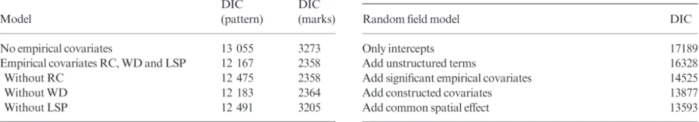
Separate DIC-values for the pattern and the marks gained from running models with the intercepts, the unstructured fields and different subsets of the empirical covariates are given in Table 1. For the intensity of the pattern, we notice that all the empirical covariates are relevant to the model as the DIC increases if any of these terms are left out. However, there is no evidence thatR. monosperma cover directly impacts on the health status of the plants.
Significance of the empirical covariates may also be assessed by calculating posterior means, standard deviations and credi-ble intervals for each term (see Tacredi-ble 2). These results support the conclusions already made. The negative posterior mean indicates thatR. monospermacover has a negative impact on the location of the T. carnosus plants; this is reasonable because only few T. carnosus plants grow underneath R. monosperma plants. However, the competitive effect of R. monospermais not significant for the health status of the T. carnosusplants and is hence not considered in the final model. Hence, competition withR. monospermaimpacts on the long-term establishment of the plants in the environment, but it does not impact on short-term survival.
The distance to the water-table has a positive significant effect on both the location and the health status of the T. carnosusplants. This indicates that the density ofT. carnosus plants is higher in areas where the water-table is low and that these plants are also healthier. The level of livestock pressure (LSP) is seen to impact on both the intensity of the pattern and
on the health status of the plants as all credible intervals for dif-ferent levels of LSP are significantly different from 0 (results not shown). However, to more fully account for random struc-ture due to different study regions, and to provide a better understanding of spatial processes in the data, spatially struc-tured effects should also be included in the model.
A D D IN G C O N S T R U C T E D CO V A R IA T E S A N D S P A T IA L E F F E C T S
We now add constructed covariates and a joint spatially struc-tured effect to account for local clustering and random large-scale variation impacting on short- and long-term survival, respectively, not explained by the empirical covariates. As mentioned, these effects might easily be overfitted to the actual pattern making the empirical covariates in the model redun-dant. Thus, the prior parameters for these effects need to be chosen carefully to avoid overfitting. We choose to estimate joint spatial effects for the pattern and the marks, for each of the given plots.
Table 3 summarizes the DIC-values for various joints model for the pattern and the marks as the different terms are added to the model. The final model with the lowest DIC, using a common spatial effect, is the following:
gð1Þijk ¼b01þb11RCðsijkÞ þb21WDðsijkÞ þLSPkþfðzcðsijkÞÞþ
fksðsijkÞ þuðsijkÞ
eqn 5 gð2Þijk ¼b02þb22WDðsijkÞ þLSPkþbsfksðsijkÞ þvðsijkÞ
eqn 6
in which the estimated value ofbsis 1343. The constructed covariate is significant for the pattern, but the model fit does Table 1.Separate DIC values for pattern and marks including
inter-cepts, empirical covariates and error fields; RC refers toRetama mono-spermacover, WD to the distance from the terrain to the water level and LSP to livestock pressure
Model
DIC (pattern)
DIC (marks)
No empirical covariates 13 055 3273 Empirical covariates RC, WD and LSP 12 167 2358
Without RC 12 475 2358
Without WD 12 183 2364
Without LSP 12 491 3205
Table 2. Posterior mean, standard deviation and 95% pointwise credi-ble intervals for fixed effects; RC refers toRetama monospermacover and WD to the distance from the terrain to the water level
Mean SD
25% quant.
975% quant.
Intercept for pattern b01 0828 0109 1047 0618
RC for pattern b11 1007 0056 1117 0898
WD for pattern b21 0096 0023 0051 0143
Intercept for marks b02 0402 0306 0203 0998
RC for marks b12 0266 0175 0606 0079
WD for marks b22 0180 0066 0052 0311
Table 3. Summary of DIC values for joint models of the pattern and marks, having increasing complexity
Random field model DIC
Only intercepts 17189
Add unstructured terms 16328
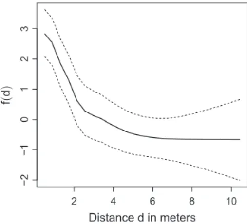
not improve if it is included in the model for the marks. Figure 1 shows the estimated functional relationship between the constructed covariate and the spatial pattern. The plot reveals that the plants are locally clustered (up to around 2 m), as the curve shows that the intensity of the pattern is high if the constructed covariate, i.e. the distance to the nearest neighbour, is low. The same constructed co-variate is non-significant for the health status resulting in a flat curve (result not shown). In other words, the model does not indicate that the health status is worse or better in areas where the pattern is locally clustered than in areas where the plants do not cluster locally.
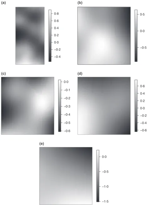
Figure 2 shows the estimated common spatially structured effect, i.e. residual spatial autocorrelation unexplained by the covariates, for each of the plots. As these are clearly exhibiting a structure that is not flat or uniform in space, they reveal that the residual spatial autocorrelation is present in the data that cannot be explained by the covariates alone. A careful inspec-tion of these surfaces might serve as a means of identifying additional covariates that might improve the model and impact on the establishment ofT. carnosusplants.
For more specific results, we may consider the posterior dis-tribution for the explanatory variables. The posterior means as well as standard deviations and 95% credible intervals for the intercepts, the degree ofR. monospermacover and the distance to the water-table in the final model, are summarized in Table 4. We notice that the empirical covariates are still signifi-cant after the constructed covariate and the spatial effect have been added. The effect of livestock pressure on the intensity of the pattern and on the marks (posterior mean and 95% credi-ble intervals) is illustrated in Fig. 3. Livestock pressure clearly has a strong effect on the health status of the plants. Not sur-prisingly, plants seem to be healthier at a low level of livestock pressure while a high level of livestock pressure worsens the health status. The non-herbivory plots (‘Nat’) are non-accessi-ble for livestock, but have a high percentage ofR. monosperma cover and the number ofT. carnosusplants here is lower than in the other plots.
Discussion
In this contribution, we have highlighted the potential for using an emerging statistical methodology, INLA, within the context of spatial ecological data. We have explained how it promises to facilitate the analysis of more complex spatial data sets than has to date been possible and have demonstrated this potential using a typically complex data set of spatial plant dis-tributions that, in this case, includes individual health status as well as spatial covariates. We anticipate that INLA will have two major impacts on the inferences we make from spatial eco-logical data. The first is that it promises to substantially improve the robustness of the sorts of inferences that we are already making; this is because it enables the real complexity that exists in many ecological data sets to be more fully incor-porated. The second benefit is that it will make new inferences possible that could not have been considered previously. In particular, these are likely to relate to gaining insights into pro-cesses and patterns that operate simultaneously or at different levels of a system such as the different temporal scales in the study data set. Similarly, several types of data that inform on the same or related processes may be analysed in one inte-grated model. This includes situations where data are available from a number of sources with a different quality and we can substantially gain from jointly exploiting all the information contained in these.
In this discussion, we will first provide some relatively brief ecological interpretation of the results gained for our case study before turning to the main focus of the article, which is the application of INLA in spatial ecological analy-sis in general. Here, we will describe the current state of the statistical field and explain what is and what is not currently possible using INLA and suggest some promising potential avenues where ecological analysis may progress rapidly using the currently available methods. Finally, we will high-light where further work between ecologists and statisticians will be required to develop the methodology such that it is able to deal with an even greater range of spatial ecological data sets.
ECOLOGICAL DISC USSION
Our analysis of the marked point pattern (i.e. the spatial distri-bution of plants according to health status) yields some clear results. It confirms thatT. carnosusis found much less fre-quently in the proximity ofR. monosperma(underR. mono-spermacanopy). Given our expectation thatR. monospermais a strong competitor, it is not surprising that we find substan-tially reduced densities ofT. carnosusnearR. monosperma. In addition, in sites with higher livestock disturbance, we believe the reducedT. carnosusdensity under the canopy, is due to a trampling effect of the livestock which are often located in the proximity of theR. monosperma. In terms of health status, we find no effect ofR. monospermapresence onT. carnosus. This suggests that, in a particularly dry year,R. monosperma pres-ence does not have a short-term impact on localT. carnosus plants. From this result, we might hypothesize that the longer
2 4 6 8 10
−
2
−
10
1
2
3
Distance d in meters
f
(
d
)
term negative effect ofR. monospermaonT. carnosus(that we do observe in the data) is perhaps more due to competition for light rather than competition for water.
The most interesting result revealed by our spatial analysis relates to the distance-to-water covariate: while T. carnosus plants are typically at higher density close to water, they are generally healthier when they are further from the water. The Mediterranean-type climate is characterized not only by a strong seasonal variability of rainfall, with cool, wet winters and hot, dry summers, but with unpredictable alternating years of severe drought with others of high precipitation rates. So, following an unusually dry year, we observe higher mortality of individuals that are growing closer to the water-table, a result that, at first sight, seems counterintuitive and warrants some explanation. In common with all other species occupying the harsh environment represented by the Mediterranean dunes, T. carnosus has to be well-adapted to water stress which, especially during summer, can be substantial. Plants liv-ing in such water-limited ecosystems have evolved a range of rooting strategies that enable them to avoid serious water-−0·4
−0·2 0·0 0·2 0·4 0·6 0·8
−0·5 0·0 0·5 (b)
(a)
−0·6 −0·5 −0·4 −0·3 −0·2 −0·1 0·0
−0·6 −0·4 −0·2 0·0 0·2 0·4 0·6 (d)
(c)
−1·5 −1·0 −0·5 0·0 (e)
Fig. 2.Estimated common spatial trend for the spatial pattern and marks (posterior mean) in each of the five plots.
Table 4.Posterior mean, standard deviation and 95% pointwise credi-ble intervals for fixed effects of the final model; RC refers toRetama monospermacover and WD to the distance from the terrain to the water level
Mean SD
25% quant.
975% quant.
Intercept for pattern b01 3214 0432 4085 3206
RC for pattern b11 0404 0059 0521 0404
WD for pattern b21 0066 0028 0013 0065
Intercept for marks b02 0332 0366 0389 0333
deficit (Larcher 1995; Rodriguez-Iturbeet al.2001; Collins & Bras 2007; Viola et al. 2008); these include both intensive exploitation strategies involving roots and transpiration systems that rapidly respond to intermittent and unpredictable rainfall events during the summer months and extensive exploitation strategies with roots that extend deeper and enable individuals to benefit from soil moisture at much greater depths. Many species are characterized as utilizing mainly one of these rooting strategies (Violaet al. 2008; Jeneretteet al. 2012), such as dimorphic root systems (Dawson & Pate 1996). However,T. carnosusis quite plastic and can use both strate-gies to a greater or lesser extent depending upon local environ-mental conditions. In the absence of a water-table near the surface, the species typically develops a root system capable of taking water from precipitation or condensation on the surface of soil (a more intensive strategy). However, when groundwa-ter is close (<15 m), the radical system ofT. carnosusis dimor-phic, with some shallow roots but also deeper roots that can reach groundwater. We hypothesize that the plasticity in root-ing strategy provides the likely explanation for our observation that the plants growing closer to the water-table are the ones to suffer the most from an unusually dry summer. We suggest that these individuals are likely to be much more reliant on the deeper water accessed by their extensive rooting system and have invested much less heavily in an intensive rooting system that would equip them to access the water available near the surface from light precipitation or condensation. So, when the water-table drops, they are likely to be prone to suffer a much greater water-deficit than those individuals with a more inten-sive rooting system that do not rely on the deeper water. This type of rooting strategy would correspond with the response found by Zunzunegui, Caldeira-Dıaz-Barradas & Novo (2000) in another Mediterranean species, Halimium halimifolium. Even though water-table was further away for plants at the top of the dune, Halimium halimifolium plants from this site exhibited better physiological and vegetative responses than Halimium halimifoliumplants growing in the dune slack. It was suggested that these individuals acclimated to permanent water availability could show higher sensitivity to drought events than the former, which never reached the water-table. Our result provides an interesting example of how plastic responses
to spatially heterogeneous environmental conditions may make the response of individuals to environmental stress inher-ently hard to predict.
METHOD OLOGIC A L DISCU SS ION
In this article, we discuss a marked spatial point process model and jointly fit this model to both the spatial pattern formed by individual plants and the associated marks. Using INLA enables us to fit this complex point process model at relatively little computational cost, while it would be computationally prohibitive to do this with standard MCMC methods (see Rue, Martino & Chopin 2009 for comparisons of running times). In addition, the full model and appropriate submodels may be considered to allow for model comparison. Certainly, INLA may be applied to fit many other complex point process models. This includes other marked point processes such as multivariate models, and models with marks following other distributions, such as normal for continuous marks, Poisson for count data, zero-inflated Poisson, etc. Similarly, INLA also facilitates the integrated analysis of other joint models such as models of a spatial pattern and spatial covariates that account for measurement error in the covariates (Illian, Sørbye & Rue 2012) or spatio-temporal point patterns. The latter constitute an emerging field within statistics (Diggle 2007) and this prom-ises to open even more opportunities for analysis of ecological data.
In discussing the data example here, we aim at introducing an ecological audience to spatial modelling based on INLA fit-ting a latent Gaussian model, in particular a marked Cox pro-cess model to an ecological data set. Many spatial point process models, including Poisson models (Aarts, Fieberg & Matthiopoulos 2012) and Gibbs process models (Baddeley & Turner 2005) do not assume a latent random model, but use models that are based on a deterministic trend. Modelling the spatial trend in these models hence often assumes that an explicit and deterministic model of the trend as a function of location (and spatial covariates) is known (Baddeley & Turner 2005). The estimated values of the underlying spatial trend are considered fixed values, which are subject neither to stochastic variation nor to measurement error. As it is based on a latent Nat
Low High
−
1·0
−
0·5
0·0
0·5
−
2
−
10
1
2
Nat Low
High
(b) (a)
random field, the approach discussed here differs from these approaches in assuming a hierarchical, doubly stochastic struc-ture. This provides a flexible class of point processes models which assume that the spatial trends exist in the data that can-not be accounted for by the covariates. The spatial trend is hence not regarded as deterministic, but assumed to be a random field.
In general, analysing the spatial pattern formed by individu-als in space is not necessarily the interest of all ecological stud-ies involving spatial data and hence point process models are certainly only one type of spatial model that is relevant here. As the class of latent Gaussian models is very general, many other spatial (and indeed non-spatial) data structures may be fitted with INLA. For instance, similar modelling techniques may also be applied to geostatistical data, i.e. a situation where the aim is to fit a spatially continuous model to measurements taken at a finite number of discrete locations (Diggle & Ribeiro 2007). This includes situations where preferential sampling is likely to have occurred (Diggle, Menezes & Su 2010). Similarly, models for data that have been collected on a–regular or irreg-ular–spatial grid can also be fitted taking a strongly related approach to the model discussed here (Rue & Held 2005). In other words, while we discuss one specific example here, the INLA methodology is generally applicable to many other spatial models.
It is worth mentioning that many other complex data struc-tures that are not necessarily spatial may be fitted with INLA– in a Bayesian setting. Examples include models with random effects, dynamic linear models, stochastic volatility models, generalized linear (mixed) models, generalized additive (mixed) models, spline smoothing, semiparametric regression, space-varying (semiparametric) regression models, disease mapping, spatio-temporal models, survival models etc. (see Rue, Martino & Chopin 2009). While INLA facilitates the fitting of increasingly complex models, there will inevitably be eventual limitations. In particular, an increase in the number of hyperparameters will eventually also slow down INLA.
The current approach uses a regular spatial grid and approx-imates both the latent field and the spatial pattern by this grid. Due to this, a dense lattice has to be used to be as exact as possible. Recent statistical developments that approximate the random field by the solution to a stochastic differential equa-tion (SPDE) defined on a triangulaequa-tion avoid these issues. Here, the resolution of the spatial component can be locally controlled (Lindgren, Rue & Lindstro¨m 2011). Combining this SPDE approach with INLA is currently undergoing develop-ment. This will allow for more flexible models to be fitted since the spatial field and hence the latent process may be defined to account for phenomena relevant in realistic data sets such as varying boundary conditions or observation windows with holes (Simpsonet al.2011).
In summary, INLA already provides considerable oppor-tunities for the fitting of spatial ecological data that would previously have been impossible to fit using other approaches. Although most often ecologists will apply newly emerging statistical methods some time (often some consider-able time) after they have been initially developed by the
stat-isticians, the development and application of the methods can, in this case, benefit substantially from the close working together of spatial ecologists and statisticians. There are many ways in which INLA can be further developed such that it is able to be used for analysis of a greater range of spa-tial data and ecologists with an intimate knowledge of their data, and of the key questions they want to explore using their data, can help to prioritize the directions future statisti-cal developments take. The ecologists benefit by having meth-ods available to address questions they may otherwise be unable to answer while the statisticians benefit by having access to ecological data exhibiting interesting statistical properties that may often demand the development of new statistical approaches. We hope and anticipate that over the next few years we will witness a rapid development of these statistical methods driven, at least in part, by a recognition that they offer enormous potential to provide novel insights into ecological processes through the analysis of complex spa-tial data.
References
Aarts, G., Fieberg, J. & Matthiopoulos, J. (2012) Comparative interpretation of count, presence–absence and point methods for species distribution models. Methods in Ecology and Evolution,3, 177–187.
Ales, E.E., Sanchez Gullon, E. & Pena, J. (2003) Consideraciones sobre la cate-~ gorıa de amenaza paraThymus carnosusen el suroeste de Espa~na. Conserva-cion Vegetal. Boletin de la comision de flora del comite espanol de la U.I.C.N.,8, 9–10.
Baddeley, A.J. & Turner, R. (2005) Spatstat: an R package for analyzing spatial point patterns.Journal of Statistical Software,12, 1–42.
Beale, C.M., Lennon, J.J., Yearsley, J.M., Brewer, M.J. & Elston, D.A. (2010) Regression analysis of spatial data.Ecology Letters,13, 246–264.
Brooks, S.P., King, R. & Morgan, B.J.T. (2004) A Bayesian approach to combin-ing animal abundance and demographic data.Animal Biodiversity and Conser-vation,27, 515–529.
Brown, C., Law, R., Illian, J.B. & Burslem, D. (2011) Linking ecological pro-cesses with spatial and non-spatial patterns in plant communities.Journal of Ecology,99, 1402–1414.
Cabezudo, B., Talavera, S., Blanca, G., Salazar, C., Cueto, M., Valdes, B., Hernandez-Bermejo, E., Herrera, C.M., Rodrıguez-Hiraldo, C. & Navas, D. (2005)Lista Roja de la Flora Vascular de Andalucıa. Consejerıa de Medio Ambiente, Junta de Andalucıa, Seville.
Collins, D. & Bras, R. (2007) Plant rooting strategies in water-limited ecosystems. Water Resources Research,43, W06407.
Cornulier, T. & Bretagnolle, V. (2006) Assessing the influence of environmental heterogeneity on bird spacing patterns: a case study with two raptors. Ecogra-phy,29, 240–250.
Dawson, T. & Pate, J. (1996) Seasonal water uptake and movement in root sys-tems of Australian phraeatophytic plants of dimorphic root morphology: a stable isotope investigation.Oecologia,107, 13–20.
Diggle, P. (2003)Statistical Analysis of Spatial Point Patterns, 2nd edn. Hodder Arnold, London.
Diggle, P. (2007) Spatio-temporal point processes: methods and applications. Statistical Methods for Spatio-temporal Systems(eds B. Finkenst€adt, L. Held & V. Isham), pp. 1–45. Chapman & Hall/CRC Press, Boca Raton, Florida, USA.
Diggle, P., Menezes, R. & Su, T. (2010) Geostatistical inference under preferential sampling (with discussion).Journal of the Royal Statistical Society Series C,
59, 191–232.
Diggle, P.J. & Ribeiro, P.J. (2007)Model-Based Geostatistics (Springer Series in Statistics). Springer, New York.
Gallego-Fernandez, J., Munoz Vall~ es, S. & Dellafiore, C. (2006)Flora and Vege-tation on Nueva Umbria Spit (Lepe, Huelva). Lepe Council, Lepe.
Ho, L.P. & Stoyan, D. (2008) Modelling marked point patterns by intensity-marked Cox processes.Statistical Probability Letters,78, 1194–1199. Illian, J.B., Penttinen, A., Stoyan, D. & Stoyan, H. (2008)Analysis and Modelling
Illian, J.B. & Rue, H. (2010) A toolbox for fitting complex spatial point process models using integrated Laplace transformation (INLA). Technical Report, Trondheim University.
Illian, J.B., Sørbye, S.H. & Rue, H. (2012) A toolbox for fitting complex spatial point process models using integrated nested Laplace approximation (INLA). Annals of Applied Statistics,6, 1499–1530.
Illian, J.B., Sørbye, S.H., Rue, H. & Hendrichsen, D.K. (2012) Fitting a log Gaus-sian Cox process with temporally varying effects – a case study.Journal of Environmental Statistics,3, 1–25.
Jenerette, G., Barron-Gafford, G., Guswa, A., McDonnell, J. & Villegas, J. (2012) Organization of complexity in water limited ecohydrology. Ecohydrolo-gy,5, 184–199.
King, R., Morgan, B.J.T., Gimenez, O. & Brooks, S.P. (2009)Bayesian Analysis for Population Ecology. CRC Press, Boca Raton, Florida, USA.
Larcher, W. (1995)Physiological Plant Ecology. Springer, Berlin.
Law, R., Illian, J.B., Burslem, D.F.R.P., Gratzer, G., Gunatilleke, C.V.S. & Gunatilleke, I.A.U.N. (2009) Ecological information from spatial patterns of plants: insights from point process theory.Journal of Ecology,97, 616–628. Lin, Y., Chang, L., Yang, K., Wang, H. & Sun, I. (2011) Point patterns of tree
dis-tribution determined by habitat heterogeneity and dispersal limitation. Oecolo-gia,165, 175–184.
Lindgren, F., Rue, H. & Lindstro¨m, J. (2011) An explicit link between Gaussian fields and Gaussian Markov random fields: the SPDE approach.Journal of the Royal Statistical Society, Series B,73, 423–498.
Martınez, I., Wiegand, T., Gonzalez-Taboada, F. & Obeso, J.R. (2010) Spatial associations among tree species in a temperate forest community in north-wes-tern Spain.Forest Ecology and Management,260, 456–465.
Møller, J., Syversveen, A.R. & Waagepetersen, R.P. (1998) Log Gaussian Cox processes.Scandinavian Journal of Statistics,25, 451–482.
Møller, J. & Waagepetersen, R.P. (2004)Statistical Inference and Simulation for Spatial Point Processes. Chapman & Hall/CRC, Boca Raton, Florida, USA.
Møller, J. & Waagepetersen, R.P. (2007) Modern statistics for spatial point pro-cesses (with discussion).Scandinavian Journal of Statistics,34, 643–711. Mu~noz Valles, S., Gallego-Fernandez, J. & Dellafiore, C. (2009) Estudio florıstico
de la flecha litoral de el rompido (lepe, huelva) analisis y catalogo de la flora vascular de los sistemas de duna y marisma.Lagascalia,29, 43–88.
Mu~noz Valles, S., Gallego-Fernandez, J., Dellafiore, C. & Cambrolle, J. (2011) Effects on soil, microclimate and vegetation of the native-invasiveRetama monosperma(L.) in coastal dunes.Plant Ecology,212, 169–179.
Myllym€aki, M. & Penttinen, A. (2009) Conditionally heteroscedastic intensity-dependent marking of log Gaussian Cox processes.Statistica Neerlandica,63, 450–473.
Neeff, T., Biging, G.S., Dutra, L.V., Freitas, C.C. & dos Santos, J.R. (2005) Mar-kov point processes for modeling of spatial forest patterns in Amazonia derived from interferometric height.Remote Sensing of Environment,97, 484– 494.
Parra, R., Valdes, B., Oca~na, M.E. & Dıaz Lifante, M.J. (2000)Thymus carnosus Boiss.Libro Rojo de la Flora Silvestre Amenazada de Andalucıa, Tomo II,11, 355–357.
Perry, G.L.W., Enright, N.J., Miller, B.P. & Lamont, B.B. (2008) Spatial patterns in species-rich sclerophyll shrublands of southwestern Australia.Journal of Vegetation Science,19, 705–716.
Reynolds, T.J., King, R., Harwood, J., Frederikesen, M., Harris, M.P. & Wan-less, S. (2009) Integrated data analyses in the presence of emigration and
tag-loss.Journal of Agricultural, Biological, and Environmental Statistics,14, 411– 431.
Rodriguez-Iturbe, I., Porporato, A., Laio, F. & Ridolfi, L. (2001) Intensive or extensive use of soil moisture: plant strategies to cope with stochastic water availability.Geophysical Research Letters,28, 4495–4497.
Rue, H. & Held, L. (2005)Gaussian Markov Random Fields. Chapman & Hall/ CRC, Boca Raton, Florida, USA.
Rue, H., Martino, S. & Chopin, N. (2009) Approximate Bayesian inference for latent Gaussian models by using integrated nested Laplace approximations (with discussion).Journal of the Royal Statistical Society B,71, 319–392. Schiffers, K., Schurr, F.M., Tielb€orger, K., Urbach, C., Moloney, K. & Jeltsch,
F. (2008) Dealing with virtual aggregations–a new index for analysing hetero-geneous point patterns.Ecography,31, 545–555.
Simpson, D., Illian, J., Lindgren, F., Sørbye, S.H. & Rue, H. (2011) Going off grid: computationally efficient inference for log-Gaussian Cox processes. Tech-nical Report, Trondheim University.
Spiegelhalter, D.J., Best, N.G., Carlin, B.P. & van der Linde, A. (2002) Bayesian measures of model complexity and fit (with discussion).Journal of the Royal Statistical Society, Series B,64, 583–616.
Viola, F., Daly, E., Vico, G., Cannarozzo, M. & Porporato, A. (2008) Transient soil-moisture dynamics and climate change in mediterranean ecosystems. Water Resources Research,44, W11412.
Wang, X., Wiegand, T., Hao, Z., Li, B., Ye, J. & Lin, F. (2010) Species associa-tions in an old-growth temperate forest in north-eastern China.Journal of Ecology,98, 674–686.
Wiegand, T. & Moloney, K. (2004) Rings, circles, and null-models for point pat-tern analysis in ecology.Oikos,104, 209–229.
Wiegand, T., Gunatilleke, S., Gunatilleke, N. & Okuda, T. (2007) Analysing the spatial structure of a Sri Lankan tree species with multiple scales of clustering. Ecology,88, 3088–3012.
Zhang, J., Song, B., Li, B.-H., Ye, J., Wang, X.-G. & Hao, Z.-Q. (2010) Spatial patterns and associations of six congeneric species in an old-growth temperate forest.Acta Oecologica,36, 29–38.
Zunzunegui, M., Caldeira-Dıaz-Barradas, M.C. & Novo, F.G. (2000) Different phenotypic response ofHalimium halimifoliumin relation to groundwater availability.Plant Ecology,148, 165–174.
Zunzunegui, M., Esquivias, M.P., Oppo, F. & Gallego-Fernandez, J.B. (2012) Interspecific competition and livestock disturbance control the spatial pattern of two coastal dune shrubs.Plant and Soil,354, 299–309.
Received 15 November 2011; accepted 4 October 2012 Handling Editor: David Warton
Supporting Information
Additional Supporting Information may be found in the online version of this article.