CEC Theses and Dissertations College of Engineering and Computing
2015
Feature Selection and Classification Methods for
Decision Making: A Comparative Analysis
Osiris Villacampa
Nova Southeastern University,[email protected]
This document is a product of extensive research conducted at the Nova Southeastern UniversityCollege of Engineering and Computing. For more information on research and degree programs at the NSU College of Engineering and Computing, please clickhere.
Follow this and additional works at:http://nsuworks.nova.edu/gscis_etd
Part of theBusiness Intelligence Commons,Management Information Systems Commons, Management Sciences and Quantitative Methods Commons,Technology and Innovation Commons, and theTheory and Algorithms Commons
Share Feedback About This Item
This Dissertation is brought to you by the College of Engineering and Computing at NSUWorks. It has been accepted for inclusion in CEC Theses and Dissertations by an authorized administrator of NSUWorks. For more information, please [email protected].
NSUWorks Citation
Osiris Villacampa. 2015.Feature Selection and Classification Methods for Decision Making: A Comparative Analysis.Doctoral dissertation. Nova Southeastern University. Retrieved from NSUWorks, College of Engineering and Computing. (63)
Feature Selection and Classification Methods for Decision Making: A
Comparative Analysis
By
Osiris Villacampa
A dissertation submitted in partial fulfillment of the requirements for the Degree of Doctor of Philosophy
In
Information Systems
College of Engineering and Computing Nova Southeastern University
iii
An Abstract of a Dissertation Report Submitted to Nova Southeastern University in Partial Fulfillment of the Requirements for the Degree of Doctor of Philosophy
Feature Selection and Classification Methods for Decision Making: A
Comparative Analysis
by
Osiris Villacampa August 2015
The use of data mining methods in corporate decision making has been increasing in the past decades. Its popularity can be attributed to better utilizing data mining algorithms, increased performance in computers, and results which can be measured and applied for decision making. The effective use of data mining methods to analyze various types of data has shown great advantages in various application domains. While some data sets need little preparation to be mined, whereas others, in particular high-dimensional data sets, need to be preprocessed in order to be mined due to the complexity and inefficiency in mining high dimensional data processing. Feature selection or attribute selection is one of the techniques used for dimensionality reduction. Previous research has shown that data mining results can be improved in terms of accuracy and efficacy by selecting the attributes with most significance. This study analyzes vehicle service and sales data from multiple car dealerships. The purpose of this study is to find a model that better classifies existing customers as new car buyers based on their vehicle service histories. Six different feature selection methods such as; Information Gain, Correlation Based Feature Selection, Relief-F, Wrapper, and Hybrid methods, were used to reduce the number of attributes in the data sets are compared. The data sets with the attributes selected were run through three popular classification algorithms, Decision Trees, k-Nearest Neighbor, and Support Vector Machines, and the results compared and analyzed. This study concludes with a comparative analysis of feature selection methods and their effects on different classification algorithms within the domain. As a base of comparison, the same procedures were run on a standard data set from the financial institution
Dedication
This dissertation is gratefully dedicated to my late mother Sylvia Villacampa. Thanks for teaching me that all goals are attainable with hard work and dedication.
Acknowledgements
I would like to extend my sincere and heartfelt gratitude towards all the individuals who have supported me in this endeavor. Without their guidance, advice, and
encouragement, I would have never finished.
I would like thank my advisor, Dr. Sun, for his guidance, direction, patience, and continuous encouragement throughout the time of my dissertation research. He was always there to answer my questions and set time to meet with me whenever needed. I will be forever grateful.
I would also like to thank my committee members, Dr. Nyshadham and Dr. Zhou, whose comments, advice, and suggestions from idea paper to final report were valued greatly.
I would also like to thank my sister, Dulce. She will always be my role model and muse. Thanks to my children, Alexis and Osiris, who were always supporting me and reminding me of the ultimate goal.
Finally, I would like to thank my wife, Maria. Her words of encouragement and support are what kept me going all these years.
vi
Table of Contents
Abstract iii List of Tables viii List of Figures xi Chapters
1. Introduction 1 Background 1
Statement of Problem and Goal 3 Relevance and Significance 5 Barriers and Issues 6
Definition of Terms 7
Organization of the Remainder of the Dissertation Report 7 2. Review of Literature 9 Feature Selection 12 Data Mining 18 Performance Measures 25 3. Methodology 34 Introduction 34
Data Mining Process 34 Data 37 Data Acquisition 37 Data Pre-Processing 40 Feature Selection 44 Classification Algorithms 52 Performance Evaluation 74 Apparatus 84 Data Sets 85 Summary 87 4. Results 89 Introduction 89 Bank Data Set 89 Service Data Set 109 Summary 124
vii
5. Conclusions, Implications, Recommendations, and Summary 125 Introduction 125 Conclusions 126 Implications 128 Recommendations 128 Summary 129 Appendixes A. Data Schema 132 B. Data Dictionaries 133
C. WEKA Functions and Parameters 149 D. All Classification Results 155
Reference List 161 Bibliography 170
viii
List of Tables
Tables
1. Confusion Matrix 26
2a. Confusion Matrix for a Perfect Classifier 28 2b. Confusion Matrix for Worst Classifier 28
2c. Confusion Matrix for an Ultra-Liberal Classifier 28 2d. Confusion Matrix for an Ultra-Conservative Classifier 29 3. Quinlan (1986) Golf Data Set 47
4. Top 10 Attributes Ranked by Relief-F Using the UCI Bank Data Set 49
5. Performance Matrix Template 51
6. Web Data Set 55
7. Web Data Set with Distance Calculated 56 8. Data after Normalization 57
9. Data Set with Weighted Distance 58 10. Data after Discretization 61
11. Confusion Matrix for a Binary Classification Model 74 12. Bank Data Set Attributes 86
13. Top 15 Attributes Ranked by Information Gain by Using the UCI Bank Data Set 90
14. Top 15 Attributes Ranked by Relief-F by Using the UCI Bank Data Set 91 15. Attributes Selected by CFS by Using the UCI Bank Data Set 92
16. Results after Applying the Wrapper Selection by Using the UCI Bank Data Set 93 17. Performance of the Decision Tree Classifier across the UCI Bank Data Set in Terms
ix
18. Confusion Matrix for Decision Tree Algorithm Using J48 Wrapper Data Set 96 19. Performance Measures for Decision Tree Algorithm Using J48 Wrapper Data Set
96
20. Performance of the J48 Classifier across the UCI Bank Data Set in Terms of Accuracy AUC, TP Rate, and FP Rate Evaluation Statistics for Different Confidence Factors 97
21. Performance of the Decision Tree Classifier across the UCI Bank Data Set in Terms of Accuracy, AUC, F-Measure, TP Rate, and TN Rate Evaluation Statistics Using a Parameter Search 98
22. Confusion Matrix for Decision Tree with Optimized Parameter Wrapper Data Set 99
23. Performance Measures for Decision Tree with Optimized Parameter Wrapper Data Set 99
24. Performance of the K-NN Classifier across the UCI Bank Data Set in Terms of Accuracy, AUC, F-Measure, TP Rate, and TN Rate Evaluation Statistics 100 25. Confusion Matrix for Nearest Neighbor Using k = 5 101
26. Performance Measures for Nearest Neighbor Using k = 5 102
27. Performance of the Lib-SVM Classifier across the UCI Bank Data Set in Terms of Accuracy, AUC, F-Measure, True Positive Rate, and True Negative Rate
Evaluation Statistics 103
28. Average Overall Classification Accuracy on Bank Data Set Based on Individual Runs 105
29. Accuracy Results Using Optimized Parameters by Using Experimenter 106 30. AUC Results Using Optimized Parameters by Using Experimenter 106 31. F-Measures Results for Bank Data Set Using Optimized Parameters by Using
Experimenter 107
32. Attributes Ranked Using Information Gain Method across the Service Data Set 109
33. Attributes Ranked by the Relief-F Method across the Service Data Set 110 34. Attributes Selected by CFS Method by Using the Service Data Set 111
x
35. Features Selected by Wrapper Selection by Using Service Data Set 112
36. Performance of the Decision Tree Classifier across the Service Data Set in Terms of Accuracy, AUC, F-Measure, TP Rate, and TN Rate Evaluation Statistics 113 37. Decision Tree Confusion Matrix 114
38. Decision Tree Performance Measures 115
39. Performance of the K-NN Classifier across the Service Data Set in Terms of Accuracy, AUC, F-Measure, TP Rate, and TN Rate Evaluation Statistics 116 40. Confusion Matrix for Nearest Neighbor Using k = 1 and Wrapper Data Set 117 41. Performance Measures for Nearest Neighbor Using k = 1 and Wrapper Data Set
118
42. Performance of the LIB-SVM Classifier across the Service Data Set in Terms of Accuracy, AUC, F-Measure, TP Rate, and TN Rate Evaluation Statistics with Default Parameters 118
43. Performance of the Lib-SVM Classifier across the Service Data Set in Terms of Accuracy AUC, F-Measure, TP Rate, and TN Rate Evaluation Statistics Grid Search Parameters 119
44. Average Overall Classification Accuracy on Service Data Set across All Classifiers and Feature Selection Methods through Individual Testing 120
45. Average Overall Classification Accuracy by Using Service Data Set across All Classifiers and Feature Selection Methods Using Optimized Parameters 121 46. Average Overall AUC on Service Data Set across All Classifiers and Feature
Selection Methods Using Optimized Parameters 122
47. F-Measures Results for Service Data Set with Optimized Parameters Using Experimenter 123
xi
List of Figures
Figures
1. KDD Process 11
2. Feature Selection Process 13 3. K-Nearest Neighbor with k = 3 19 4a. Linear Support Vector Machine 24 4b. Radial Support Vector Machine 24
5. Receiver Operating Characteristic Curve Points 30 6. Receiver Operating Characteristic Curves 31
7. Area Under Receiver Operating Characteristic Curve (AUC) 32
8. Framework Used in this Research 36
9. Data Acquisition Flow 39
10. K-NN Visualization with k = 3 53 11. Final Decision Tree 62
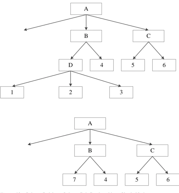
12. Subtree Raising - Subtree D is Replaced by a Single Node 64 13. Support Vector Machine for a Binary Class 67
14a. SVM Optimized by Grid Search of Parameters 70 14b. Grid Search with a Decrease in C Value 71 15. 5-Fold Cross-Validation 73
16. Classification Flow with WEKA’s KnowledgeFlow 78 17. WEKA Multiple ROC Workflow 80
18. Multiple Receiver Operating Characteristic Curves for IBK – KNN, J48 – C4.5 Decision Tree, and LibSVM – SVM Classifiers 82
xii
20. Performance of J48 Classifier across Different Feature Sets by Using the Service Data Set in Terms of Accuracy, AUC, F-Measure, TPR, and TNR Evaluation Statistics 95
21. Decision Tree Pruning. Lower Confidence Factor Indicates Higher Pruning 98 22. Performance of K-NN Classifier across Different Feature Sets Using the Service
Data Set in Terms of Accuracy, AUC, F-Measure, TPR, and TNR Evaluation Statistics 101
23. Performance of SVM Classifier across Different Feature Sets by Using the Service Data Set in Terms of Accuracy, AUC, F-Measure, TPR, and TNR Evaluation Statistics 104
24. ROC Curve for Bank Data Set 107
25. Classification Performance on Bank Data across Data Sets 108
26. Performance of J48 Classifier across Different Feature Sets by Using the Service Data Set in Terms of Accuracy, AUC, F-Measure, TPR, and TNR Evaluation Statistics 114
27. Performance of K-NN Classifier across Different Feature Sets by Using the Service Data Set in Terms of Accuracy, AUC, F-Measure, TPR, and TNR Evaluation Statistics 117
28. Performance of SVM Classifier across Different Feature Sets Using the Service Data Set in Terms of Accuracy, AUC, F-Measure, TPR, and TNR Evaluation Statistics 120
29. Service Data ROC Curves 122
Chapter 1
Introduction
Background
Businesses are constantly looking for more methodologies to keep them competitive in today’s marketplace. The low cost of disk space and ease of data capture (i.e.,
barcodes, Radio Frequency Identification - RFID tags, and credit card swipes) have led for the storage of enormous amounts of data. The data comes from various systems in the enterprise such as, Point of Sale (POS) systems, web sites, Customer Relationship
Management (CRM) software, and more. In past decades this type of information has been stored in data-warehouses and mostly used to produce trending and historical reports using tools such as Online Analytical Processing (OLAP) and Structured Query Language (SQL) (Watson & Wixom, 2009).
Today, as computing power increases and becomes more affordable, a new trend playing an important role is to mine the data for unknown patterns and to extract data that is previously unknown that may be useful to improve the decision making process
(Fayyad, Piatetsky-Shapiro, & Smyth, 1996).
Chen, Han, and Yu (1996) state: Data mining, which is also referred to as knowledge discovery in databases, means a process of nontrivial
extraction of implicit, previously unknown and potentially useful information (such as knowledge rules, constraints, regularities) from databases. (p.866) with a goal of making it ultimately understandable.
This discovery of knowledge has been used by financial institutions, to detect fraud and Index prices (Major & Riedinger, 1992); in medical research, such as heart disease prediction (Palaniappan & Awang, 2008); and in marketing, to create tools such as market-basket analysis (Agrawal, Mannila, Srikant, Toivonen & Verkamo, 1996). Data mining, which is mistakenly used as a synonym to Knowledge Discovery in Database (KDD), is just one of the steps in the knowledge discovery process (Fayyad, 1996). In general, data mining methods can be classified as two categories: supervised and unsupervised learning methods (Han, Kamber, & Pei, 2011). In supervised learning, the algorithm uses a training data set to learn model parameters. Classification
algorithms, such as Decision Trees (Breiman, Friedman, Stone, & Olshen, 1984), Support Vector Machine (SVM) (Vapnik, 1995), and Nearest Neighbor (Cover & Hart, 1967) are all members of this group. Unsupervised learning, on the other hand, uses the data itself to build the model. Clustering algorithms are the best known of this group. A third type, semi-supervised, has also been introduced as a hybrid option. Matching the data set being studied with the appropriate data mining algorithm is one of the key factors for a
successful outcome.
As more information is collected from different sources, the likelihood of needing to work with high dimensional data sources increases. High dimensional tables or those containing more than 102 to 103 attributes are starting to be the norm (Fayyad, 1996). Some disciplines such as genomic technology have sources that contain thousands if not tens of thousands of attributes (Dougherty, Hua, & Sima, 2009).
Dealing with high dimensional databases has been a key research area in statistics, pattern recognition, and machine learning (Blum & Langley, 1997). Researchers are just now applying the same interest to commercial data sets.
Statement of Problem and Goal
While disciplines such as bioinformatics and pattern recognition have been using data mining for years, more research needs to be done on high dimensional business data. The primary goal of this study is to use a real-world example, records from auto dealerships service departments, for this research. The main objective is to identify potential buyers of new vehicles based on the service history of their current vehicles. While most of the data in other domains come from a single source, the data used in this research came from many different systems. The data to be used in this study was collected from service records of approximately 200 automobile dealerships. This kind of data was combined with customer specific data retrieved from the Customer Relationship Management (CRM) systems of these same dealerships. The end result is a highly dimensional data set that contains thousands of records. There are several problems when data mining in any of high dimensional data sets.
1. As the number of features (dimensions) increases, the computational cost of running the induction task grows exponentially (Kuo & Sloan, 2005). This curse of dimensionality, as reported by Powell (2007) and Guyon & Elisseeff (2003), affects supervised as well as unsupervised learning algorithms.
2. The attributes within the data set may also be irrelevant to the task being studied, thus affecting the reliability of the outcomes.
3. There may be correlation between attributes in the data set that may affect the performance of the classification.
Feature selection or attribute selection is a technique used to reduce the number of attributes in a high dimensional data set. By reducing the number of variables in the data set the data mining algorithm’s accuracy, efficiency, and scalability can be improved (Guyon & Elisseeff, 2003). The two main approaches to feature selection are the filtering and wrapper methods. In the filtering method the attributes are selected independently to the data mining algorithms used. Attributes deemed irrelevantly will be filtered out (John, Kohavi, & Pfleger, 1994). The wrapper method selects attributes by using the data
mining algorithm selected as a function in the evaluation process (John, Kohavi, & Pfleger, 1994).
One of the successful factors in data mining projects depends on selecting the right algorithm for the question on hand. One of the more popular data mining functions is classification (Wu, et al., 2008). For this study we have opted to use several classification algorithms, as our goal is to classify our data into two labels, referred to as binary
classification. There are different types of classification algorithms available. For the purposes of this study we have chosen C4.5, a Decision Tree algorithm, K-Nearest Neighbor (K-NN), and Support Vector Machine (SVM) algorithms.
The goal in this research is made up of five related sub-goals as follows:
1) Compare and contrast different feature selection methods against the mentioned high dimensional data set and a reference data set. Both filter and wrapper methods were applied to these data sets, and their results are compared and
analyzed. The classification accuracy achieved by each method is compared against the better feature selection method found.
2) Repeat the above procedure by using different classification methods, including C4.5, a Decision Tree algorithm, K-Nearest Neighbor (K-NN), and Support Vector Machine (SVM) algorithms.
3) Compare the accuracy of the classification algorithms by using the best attributes selected for each algorithm. All methods were tested and validated on a binary classification task.
4) Use different thresholds in the classification systems and compare the effects on accuracy. K values in K-NN, number of nodes in Decision Trees, and Cost of Error (C) and Gamma settings (𝛾) in the SVM algorithm.
5) Determine which classification algorithm and feature selection combination produces the better results in order to determine new potential car buyers.
The classification algorithms, Decision Tree, K-Nearest Neighbor, and Support Vector Machine, are selected from the top 10 most commonly used algorithms (Wu, et al., 2008).
Relevance and Significance
The application of data mining for decision making is relatively new in some real world environments. The purpose of this research was to run a comparative analysis on a real world data set not only on the feature selection methods but on different
compared to illustrate the difference in using the previously mentioned methods and algorithms.
Barriers and Issues
As in many other data mining exercises we were confronted with several obstacles. The automotive data set consists of thousands of attributes and hundreds of thousands of records. Preliminary queries ran against our data tables showed that approximately 20% of the records contained null values on critical features. The quality of the data in our data set must be improved by cleaning the noise and dealing with null values. The original data set is also composed of disparate sources. This heterogeneity was dealt in the prepossessing stage of our study. Another challenge presented in this study is the highly unbalanced dataset. This imbalance, 90% in one class vs. 10% in the other, is a result of having the majority of records in a class other than the one of interest. The data set size restriction imposed on us by the software used in this research is limited by the amount of memory available in the system. We have tried to lift this restriction by populating the test computer with 32GB of random access memory. In addition, the data set was reduced initially by random selection due to its size (thousands of records). Finally, over-fitting the data to a particular model is another obstacle that needed to be addressed. This was accomplished by implementing feature selection methods,
reasonable values for k when using the K-NN algorithm, and post pruning our decision trees.
Due to time constraints and the number of different permutations possible in our study, we restricted ourselves to comparing 6 feature selection methods (3 filter, 2 wrapper, and 1 hybrid) on 3 of the most popular classifier algorithms, Decision Trees
(C4.5), Support Vector Machines (SVM), and K-Nearest Neighbor (K-NN). The following are the definition of terms used in this dissertation:
Definition of Terms
AUC – Area under the receiver-operating-characteristic curve C45 - Decision Tree Algorithm
CRISP-DM - Cross-Industry Standard Process-Data Mining CRM – Customer Relationship Management
F-Measure – Metric used for classification accuracy KDD – Knowledge Discovery in Database
K-NN - K Nearest Neighbor
ROC – Receiver Operating Characteristic SVM - Support Vector Machine
WEKA – Waikato Environment for Knowledge Analysis
Curse of Dimensionality – A term used to describe the difficulty and increase in cost of computing as the number of features increases.
Organization of the Remainder of the Dissertation Report
Chapter 2 includes a review of literature related to the use of feature selection to increase the effectiveness of data mining models. Different methods were compared and contrasted as to their strengths and weaknesses. In addition, the data mining algorithms, classification in particular, are reviewed, discussed and compared. Current, and past research were also evaluated. It concludes with an analysis of the selected feature selection methods and classification algorithms selected for this research.
Chapter 3 proposes the methodology to be used in this research. The CRISP-DM process for knowledge discovery is discussed. Steps in the process such as preparation and cleaning of the source data will be described in detail. The pre-processing stage and transformation stage which includes feature selection are also detailed. The feature selection methods proposed are discussed and metrics used for comparison are explained. The classification algorithms selected for this study are detailed along with the tests used to analyze their effectiveness.
Chapter 4 presents and describes the results of the study. It begins with the results of applying the feature selection methods in our data sets. Once the feature sets have been reduced, a new data set is saved for each method to be used in the classification phase. Our selected classification algorithms are applied to each data set and the results are compared using different performance measures.
Chapter 5 reviews our research questions, discusses our conclusions of the research based on the results, and provides suggestions for future research.
The data schema, data dictionaries, parameters used in our workbench software, and all the classification results are presented in the Appendices.
Chapter 2
Review of Literature
In today’s competitive market, companies must make critical decisions that will affect their future. These decisions are based on current and historical data the enterprise has collected using Customer Relationship Management (CRM), Enterprise Resource
Management (ERP), websites, and legacy applications. As the dimensionality and size of the data warehouses grows exponentially, domain experts must use tools to help them analyze and make decisions in a timely manner.
Knowledge Discovery in Data (KDD)
The field of Knowledge Discovery in Databases (KDD) has grown in the past several decades as more industries find a need to find valuable information in their databases. The KDD process (Fayyad, Piatetsky-Shapiro, & Smyth, 1996) is broken down into five phases (Figure 1);
1. Selection – The first stage consists of collecting data from existing sources to be used in the discovery process. The data may come from single or multiple sources. This may be the most important stage since the data mining algorithms will learn and discover from this data.
2. Preprocessing - The main goal of this stage is to make the data more reliable. Methods used to account for missing data are analyzed and implemented. Dealing with noisy data or outliers is also part of this stage.
3. Transformation – Now that we have reliable data we can make it more efficient. The uses of feature selection methods to reduce dimensionality and feature extraction to combine features into new ones are implemented at this point. Discretization of numerical attributes and sampling of data are also common tasks performed in this stage.
4. Data Mining – Before the data is mined, an appropriate data mining task such as classification, clustering, or regression needs to be chosen. Next, one or several algorithms specific to the task, such as decision trees for classification, must be properly configured and used in the discovery of knowledge. This process is repeated until satisfying results are obtained.
5. Evaluation – The last step is the interpretation of results in respect to pre-defined goals. A determination is made if the appropriate data mining model was chosen. All steps of the process are reviewed and analyzed in terms of the final results.
This study concentrates in two critical areas of the KDD process; transformation by reducing the feature set and the data mining process.
Figure 1 . KD D Proc ess (Fayy ad e t al., 1996)
Feature Selection
As the dimensionality of data increases so does the likelihood of having attributes which are irrelevant, redundant, and noisy (Chang, Verhaegen, & Duflou, 2014). A common method of reducing the dimensionality of the data to be analyzed is to reduce the number of features or variables to a more manageable number while not reducing the effectiveness of the study.
Feature selection or variable selection consists of reducing the available features to a set that is optimal or sub-optimal and capable of producing results which are equal or better to that of the original set. Reducing the feature set scales down the dimensionality of the data which in turn reduces the training time of the induction algorithm selected and computational cost, improves the accuracy of the final result, and makes the data mining results easier to understand and more applicable (Guyon & Elisseeff, 2003; Kohavi & John, 1997). While reducing the feature set may improve the performance of most classification algorithms, especially for K-NN algorithm, it may also lower the accuracy of decision trees (Li, Zhang, & Ogihara, 2004). Since decision trees have the capability of reducing the original feature set in the tree building process, beginning the process with fewer features may affect final performance.
Dash and Liu (1997) broke down the feature selection process into four steps; generation, evaluation, stopping criterion, and validation (Figure 2).
Figure 2. Feature Selection Process (Liu & Yu, 2005)
1. The first step, generation, involves searching the space of features for the subset that is most likely to predict the class best. Since the total number of possible subsets is 2n, where n is the number of features, using all attributes becomes costly as the dimensionality of the data increases. In order to minimize cost search, algorithms have been developed that scan through the attributes in search of an optimal subset. Two common methods of traversing the space are Sequential Forward Selection and Backward Elimination. The Sequential Forward Selection begins with an empty set and adds attributes one at a time. Backward Elimination, on the other hand, begins with the entire set of attributes and starts eliminating until a stopping criterion has been met. Other variations such as a random method may be used which adds or deletes variables in its search for an optimal set (Devijer & Kittler, 1982). Other algorithms, such as; the Beam Search (BS) and
Stopping Criterion Result Validation Subset Generation Subset Evaluation Subset No Yes Original Set
Smart Beam Search (SBS) algorithms select the best k features (beam-width), then proceed to add and test additional features to each of the selected k features until a stopping criterion is met (Ladha & Deepa, 2011). In their studies, Hall and Smith (1998) determined that backward and forward elimination search methods,
although elementary, were proved to be as effective as more sophisticated ones such as Best First and Beam search algorithms (Rich & Knight, 1991).
2. The second step in the process uses a predetermined evaluation function that measures the goodness of the subset (Liu & Yu, 2005). This measurement is then used to determine the ranking of the evaluated sets, which in turn are used in the selection process. Among these functions are Information Gain, Correlation Analysis, Gini Index, and in the case of wrapper methods the induction algorithm itself.
3. The third step in the process is the stopping criterion. There are many ways in which the feature search may stop. The process may be stopped if the new feature set does not improve the classification accuracy. Other options are running a predetermined number of iterations, reaching a previously defined number of features, or selecting the top n features with the highest ranking.
4. The final step is the validation of the results against the induction algorithm selected. While not exactly being a part of the actual selection process, the authors include it as it will always follow the selection process (Liu & Yu, 2005).
Feature selection methods fall into three groups, Filter, Wrapper, and Hybrid. We will discuss each in the following sections.
Filter
The filter method of feature selection reduces the number of features using properties of the data itself independently to what learning algorithm is eventually used (John, Kohavi, and Pfleger, 1994). One advantage of applying a filter algorithm to a feature set is that the number of features used in the final induction algorithm will be reduced. Therefore not only the performance of classification algorithms will be improved, but also amount of the computer processing time will be reduced. Unlike wrapper methods, filter methods do not incorporate the final learning algorithm in their process. This independency has been reported as another benefit of using filter methods (Ladha & Deepa, 2011). Another benefit is that the same features may be used in different learning algorithms for comparative analysis. Hall and Smith (1998) reported that some filter algorithms such as Correlation-based Feature Selection (CFS) might produce results similar to or better than wrapper models on several domains. Yu and Liu (2003) also proposed a new correlation based feature selection method. In their study they showed the efficiency and effectiveness of such methods when dealing with highly dimensional data sets. However, Saeys et al. (2007) noted that filter based selection methods have the disadvantage of not interacting with the classifier algorithm eventually used. Another disadvantage reported was that most filter methods are univariate in nature, meaning that they don’t take into consideration the values of other attributes. Their study was
conducted on a highly dimensional bioinformatics data set (Saeys et al., 2007).
Hall and Holmes (2003) benchmarked the filtered based feature selection and one wrapper based method against 15 test data sets in their experiments. Their conclusion was
that filter based methods varied depending on the data set, but generally they were faster and improved the effectiveness of the classifying algorithms.
This study evaluated three different filter algorithms: two multivariate algorithms Relief-F and Correlation Based Feature Selection (CFS), and, information gain a univariate algorithm. Each method is described in the following paragraphs.
The principal behind the Relief-F algorithm (Kononenko, 1994) is to select features at random and then, based on nearest neighbors, give more weight to features that
discriminate more between classes. These features are in turn ranked based on their relevance. In their empirical study, Wang and Makedon (2004) concluded that the Relief-F algorithm produced similar results to that of other filter algorithms, such as Information Gain and Gain Ratio, when the Relief-F algorithm is used in their particular domain, gene expression data.
Correlation-based Feature Selection (CFS) algorithms looks for features that are highly correlated with the class which has no or minimal correlation with each other (Hall, 2000).
Our last feature selection algorithm is information gain (IG). IG is a method that ranks features based on a relevancy score which is based on each individual attribute. The fact that the correlation between attributes is ignored makes it a univariate method.
Comparative studies between CFS and Gain Ratio methods have been performed in the past on different data domains. Karegowda, Manjunath, and Jayaram (2010) found that using the CFS method produced better results than Gain Ratio but at a substantial cost on computer time.
Wrapper
Unlike the filter method, wrapper algorithms use a preselected induction algorithm as part of the feature selection process. As features are added or subtracted the final results are ranked as to effectiveness of the selection. Since the induction algorithm itself is used in the evaluation phase of the selection process wrapper methods tend to score better results than filter methods. Kohavi and John (1997) compared the wrappers for feature subset selection against filter methods. They concluded that relevancy of attributes contribute greatly to the performance of the learning algorithms when the algorithm is taken into consideration. However, there are some limitations to these methods. The computational cost of running the evaluation is far greater than that of filter methods and increases as the number of attributes increases. Another disadvantage of the wrapper method is the likelihood of over-fitting the data.
There are also other wrapper methods. Instead of using single method wrapper such as sequential forward selection, Gheyas and Smith (2010) proposed a new method,
simulated annealing generic algorithm (SAGA), which incorporates existing wrapper methods into a single solution. The research showed that combining methods reduced the weaknesses that were inherent to each individually.
Maldonado and Weber (2009) proposed a wrapper method based on the Support Vector Machine (SVM) classification. Their study concluded that using such method would avoid over fitting the data due to its capability of splitting the data. It also allowed the use of different Kernel functions to provide better results. One drawback noted was that their proposed algorithm used the backward elimination feature which was
Hybrid/Two Stage Design
A hybrid method that incorporates the above methods has also been proposed (Kudo & Sklansky, 1998; Bermejo, de la Ossa, Gamez, & Puerta, 2012). This method uses a filter method in the first pass to remove irrelative features and then a classifier specific wrapper method to further reduce the feature set. By reducing the feature set from n
features to a lower number k, the computation space in terms of the number of features is reduced from 2𝑛 to 2𝑘. This hybrid filter-wrapper method would retain the benefits of the wrapper model while decreasing the computational costs that would be required by using a wrapper method alone.
Data Mining
The data mining phase of the KDD process is where the discovery of patterns in the data occurs. This discovery is performed by machine learning algorithms. This study will concentrate on the classification family of learning algorithms.
Classification Algorithms
One leg of this research is in classification algorithms. The goal of classification algorithms is to learn how to assign class labels to the unseen data based on models built from training data. When only two class labels exist, the classification is said to be binary. When more than two class labels exist, the problem becomes a multiclass classification. This study was focused on binary classification problems and in the comparison of different feature selection methods and their impact on three commonly studied classifier algorithms, K Nearest Neighbor, Decision Tree, and Support Vector Machine (SVM).
K-Nearest Neighbor K-NN
K-Nearest Neighbor (K-NN) classification is one of the simplest methods available for classifying objects (Cover & Hart, 1967). The algorithm assigns a class to the object based on its surrounding neighbor’s class using a pre-determined distance function (Figure 3).
Figure 3. K-Nearest Neighbor with k = 3
The number of neighbors selected, k, is a positive odd integer, usually small, to avoid potential ties. If the value of k is 1, then the object is classified in the same class as its closest neighbor. One of the advantages of this method is that no complex training is required, an approach known as “lazy learner” or instance based learner. Kordos, Blachnick, & Strzempa (2010) showed that a properly configured K-NN may be as highly effective, if not more, than other classification algorithms.
The results of the K-NN algorithm depend on what values are used in its computation. The value, k, is the number of neighbors that will decide the class of the element in question. To avoid potential over-fitting of the data, researches have commonly used small numbers. In their studies, Cover and Hart (1967), proved that good predictions could be attained by using a value of k = 1. However, Kordos et al. (2010) reported that researchers should not confine themselves to small k values but test values in the ranges of 10 to 20 as well. Their research showed that while using a value in a higher range may take more computation time, but it may produce better results. Hamerly and Speegle (2010) proposed an algorithm that would cycle through different k values in order to minimize computational time while finding an optimum k value for the data set.
The second factor that may affect the outcome is how the distance between the elements is calculated. By default most researchers’ use the Euclidean distance, but other
calculations such as Chebyshev and Manhattan distance have also been implemented (Cunningham & Delany, 2007). Finally, in order to improve the results even more, weighting the distance calculation based on feature ranking has been studied as well (Hassan, Hossain, Bailey, & Ramamohanarao, 2008; Han, Karypis, & Kumar et al., 2001).
The advantage of using K-NN over other classification algorithms is that it is intuitive and easy to setup. However, there are several disadvantages when using the K-NN algorithm.
1. The distance function must be carefully selected and fine-tuned to achieve better accuracy. Since the distance equation is computed for all features selected,
features with higher scale values would dominate. In order to account for this, normalization of the attributes is performed before the distance is measured. 2. Data with irrelevant or correlated features must be cleaned beforehand as to not
skew the results of the process (Bhatia & Vendana, 2010).
3. Computation cost is greater than other algorithms, since the process is computed in memory the amount of memory required is high. As high speed computer and memory become more affordable, this final disadvantage is becoming less concerned.
Decision Trees
Decision Trees is one of the most commonly used methods in classification (Ngai, Xiu, & Chau, 2009). Like all classification algorithms, the methods objective is to classify a target variable based on existing attribute values. In the case of decision trees, the process is broken down into individual tests (if-then) which begin at the root node and traverse the tree, depending on the result of the test in that particular node. The tree begins at the root node. From the root node the tree branches or forks out to internal nodes. The decision to split is made by impurity measures (Quinlan, 1986). Two commonly used measures in tree construction are Information Gain and Gini Index (Chen, Wang, & Zhang, 2011). These nodes in turn will continue to split until a final node or leaf node is grown. The leaf node determines the final classification of the variable being tested. Since each node tests a specific attribute in the data set, the model is very easy to understand. Tests at each node can be done on discrete as well as
structure. The disadvantages of this method are that the tree will over-fit the data into its solution. The complexity of the tree will make the domain expert hard to follow the flow of decision making in the tree.
There are several ways to prevent over-fitting:
1. The processing of nodes can be stopped when all records belong to the same class.
2. Stop processing nodes when a predetermined threshold has been met or when all records have similar attribute values.
3. If expanding current node does not improve the information gain, then a leaf node can be introduced.
4. Other methods, such as post pruning (Witten et al., 2011), may be employed. In this case the tree is fully grown and then pruned for unnecessary branches. In their studies, Tsang et al. (2011), reported that pruning the decision trees improved the final results of the classification significantly.
There are several benefits to use decision trees. The algorithms are fast at classifying records, and easy to understand. They can handle both continuous and discrete attributes. The important attributes are easily identified by the decision maker. However, there are some disadvantages as well. Variations in data may produce different looking trees (Rokach & Maimon, 2005; Otero, Freitas, & Johnson, 2012), which are not good at predicting continuous attributes, because irrelevant attributes and noisy data may affect the tree structure (Anyanwu & Shiva, 2009). In addition, if the data set has missing attribute values, then the results of which the impurity measures computed will be affected. To circumvent this problem different methods have been introduced, such as
mean substitution and case substitution (Brown & Kros, 2003) which deal with missing values in data sets. Using this method, missing values are replaced with the mean of the given attribute and the substitutions are treated as valid observations.
When the ID3 (Iterative Dichotomiser 3) decision tree inducer was first introduced by Quinlan (1986), it did not support continuous attributes. Only categorical values were supported. Later, Quinlan(1993) introduced C4.5 which handled continuous attributes. The obstacle was overcome by discretizing the continuous data in order to perform testing at each node. Other inducers such as CART (Classification and regression trees) (Breiman et al., 1984) and SLIQ (Supervised Learning in Ques) (Metha et al. , 1996) have been introduced as well.
Decision tree classification has been studied in the medical sciences (Anunciacao et al. 2010; Ge and Wong 2008; Chen et al. 2011), text classification (Irani et al. 2010), and spam detection (Bechetti et al. 2009).
SVM
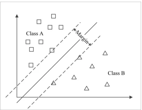
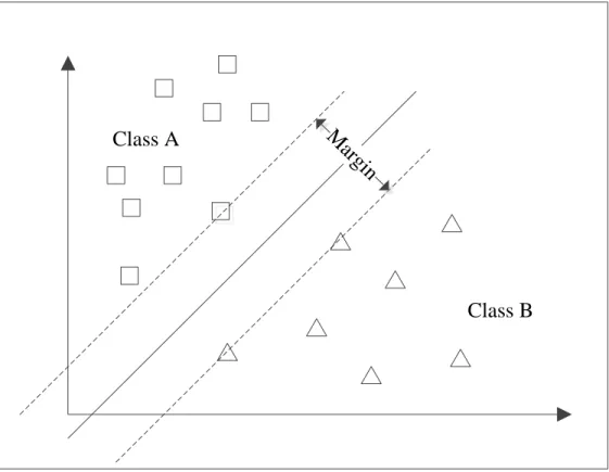
Support Vector Machines (SVM) (Vapnik, 1995) has shown great promise in binary classification (Yang & Liu, 1999). The goal of the SVM algorithm is to map the training data into a multi-dimensional feature space and then find a hyper-plane in said space that maximizes the distances between the two categories (Figure 4a-b).
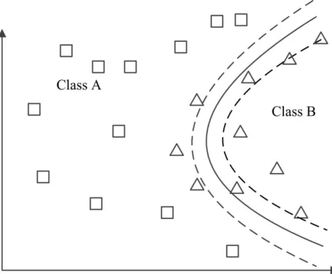
Figure 4a. Linear Support Vector Machine
Since the classifications may not be clearly separable by a linear plane non-linear kernels functions have been used (Figure 4b). Boser et al. (1992) reported that using non-linear functions proved to achieve higher performance and use less computing resources. In addition, since features with different scale may affect the results of the SVM algorithm, normalization of the numeric data is performed. In addition, normalizing the data brings the numerical data within the same scale as categorical data, that is, to a (0, 1) scale.
Performance Measures
In order to determine the effectiveness of the classification algorithm used, a
measurement is needed. Commonly used measurements include classification accuracy, F-Measure, precision, recall, Receiver Operating Characteristic (ROC) curves and Area Under the Curve (AUC) (Fawcett, 2006). These measurements can be calculated by the classification results commonly tabulated in a matrix format called a Confusion Matrix.
Confusion Matrix
In a classic binary classification problem, the classifier labels the items as either positive or negative. A confusion matrix summarizes the outcome of the algorithm in a matrix format (Chawla, 2005). In our binary example, the confusion matrix would have four outcomes:
True positives (TP) are positive items correctly classified as positive. True negatives (TN) are negative items correctly identified as negatives. False positives (FP) are negative items classified as positive.
False negatives (FN) are positives items classified as negative. Table 1 illustrates a sample confusion matrix.
Table 1. Confusion Matrix
Confusion Matrix Classified As:
Negative Positive
Actual Class
Negative TN FP
Positive FN TP
The following performance measures use the values of the confusion matrix in their calculation.
Classification Accuracy
The simplest performance measure is accuracy. The overall effectiveness of the algorithm is calculated by dividing the correct labeling against all classifications.
𝑎𝑐𝑐𝑢𝑟𝑎𝑐𝑦 = 𝑇𝑃 + 𝑇𝑁
𝑇𝑃 + 𝐹𝑃 + 𝑇𝑁 + 𝐹𝑁
The accuracy determined may not be an adequate performance measure when the number of negative cases is much greater than the number of positive cases (Kubat et al., 1998).
F-Measure
F-Measure (Lewis and Gale, 1994) is one of the popular metrics used as a performance measure. The measure itself is computed using two other performance measures, precision and recall.
𝑝𝑟𝑒𝑐𝑖𝑠𝑖𝑜𝑛 =𝑇𝑃+𝐹𝑃𝑇𝑃 𝑟𝑒𝑐𝑎𝑙𝑙 = 𝑠𝑒𝑛𝑠𝑖𝑡𝑖𝑣𝑖𝑡𝑦 = 𝑇𝑃
𝑇𝑃 + 𝐹𝑁
Precision is the number of positive examples classified over all the examples classified. Recall, also called the True Positive Rate (TPR), is the ratio of the number of positive
examples classified over all the positive examples. Based on these definitions F-measure is defined as follows:
𝑓 − 𝑚𝑒𝑎𝑠𝑢𝑟𝑒 = 2 × 𝑝𝑟𝑒𝑐𝑖𝑠𝑖𝑜𝑛 × 𝑟𝑒𝑐𝑎𝑙𝑙 𝑝𝑟𝑒𝑐𝑖𝑠𝑖𝑜𝑛 + 𝑟𝑒𝑐𝑎𝑙𝑙
In essence, the F-Measure is the harmonic mean of the recall and precision measures.
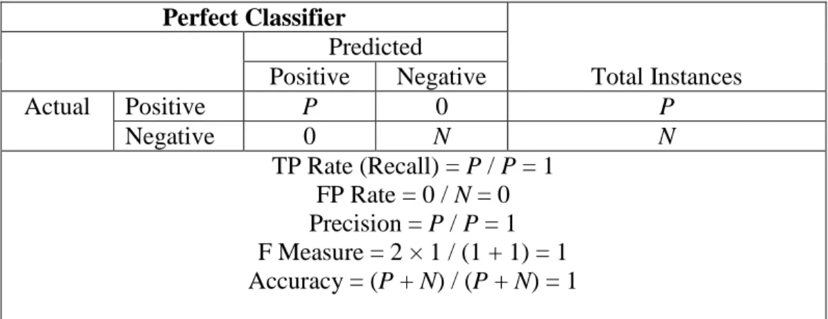
Using the confusion matrix and the performance measures mentioned above, Bramer (2007) noted four extreme cases a confusion matrix may detail:
1) A Perfect Classifier - A classifier that classifies all instances correctly. All positives are classified as positive and all negatives are classified as negative. 2) The Worst Classifier – A classifier that does not predict any positives or
negatives correctly.
3) An Ultra-Liberal Classifier – A classifier that predicts all instances as positive. 4) An Ultra-Conservative Classifier – A classifier that predicts all instances as
negative.
Tables 2a-2d show the confusion matrix for these cases along with the classification measures related to each matrix.
Table 2a. Confusion Matrix for a Perfect Classifier Perfect Classifier Total Instances Predicted Positive Negative Actual Positive P 0 P Negative 0 N N TP Rate (Recall) = P / P = 1 FP Rate = 0 / N = 0 Precision = P / P = 1 F Measure = 2 × 1 / (1 + 1) = 1 Accuracy = (P + N) / (P + N) = 1
Table 2b. Confusion Matrix for Worst Classifier Worst Classifier Total Instances Predicted Positive Negative Actual Positive 0 P P Negative N 0 N TP Rate (Recall) = 0/ P = 0 FP Rate = N / N = 1 Precision = 0 / P = 0
F Measure = Not Applicable (Precision + Recall = 0) Accuracy = 0 / (P + N) = 0
Table 2c. Confusion Matrix for an Ultra-Liberal Classifier Ultra-Liberal Classifier Total Instances Predicted Positive Negative Actual Positive P 0 P Negative N 0 N TP Rate (Recall) = P / P = 1 FP Rate = N / N = 0 Precision = P / P + N = 1 F Measure = 2 × P / (2 × P + N)
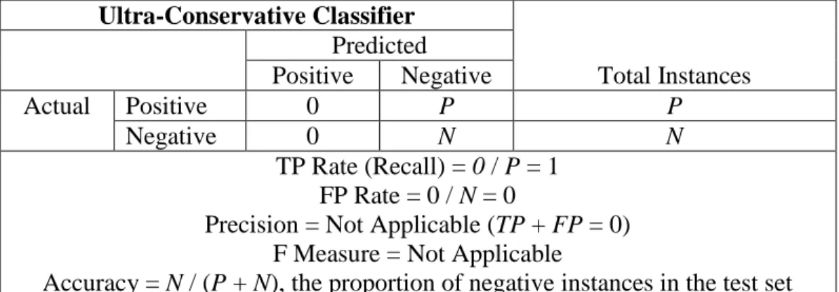
Table 2d. Confusion Matrix for an Ultra-Conservative Classifier Ultra-Conservative Classifier Total Instances Predicted Positive Negative Actual Positive 0 P P Negative 0 N N TP Rate (Recall) = 0 / P = 1 FP Rate = 0 / N = 0
Precision = Not Applicable (TP + FP = 0) F Measure = Not Applicable
Accuracy = N / (P + N), the proportion of negative instances in the test set
Sensitivity and Specificity
The performance of a binary classifier may sometimes be quantified by its accuracy as described above, i.e. the portion of misclassified classes in the entire set. However, there may be times when the types of misclassifications may be crucial in the classification assignment (Powers, 2011). In these cases, the values for sensitivity and specificity are used in determining the performance of the classifier. Sensitivity or Recall or True Positive Rate (TPR) is the ratio of true positive predictions over the number of positive instances in the entire data set.
𝑠𝑒𝑛𝑠𝑖𝑡𝑖𝑣𝑖𝑡𝑦 = 𝑇𝑃 𝑇𝑃 + 𝐹𝑁
The specificity or True Negative Rate (TNR) is the ratio of true negative predictions over the number of negative instances in the entire data set.
𝑠𝑝𝑒𝑐𝑖𝑓𝑖𝑐𝑖𝑡𝑦 = 𝑇𝑁 𝑇𝑁 + 𝐹𝑃
These values can be further analyzed using a Receiver Operating Characteristic Curve (ROC) where the sensitivity is plotted against 1- specificity (Fawcett, 2006). ROC is described further in the next section.
Receiver Operating Characteristic (ROC)
Receiver Operating Characteristic (ROC) analysis has received increasing attention in the recent data mining and machine learning literatures (Fawcett, 2006; Chawla, 2005). The graph is a plot of the false positive rate (FPR) in the X-axis and the true positive rate (TPR) in the Y-axis.
TPR = 𝑇𝑃
𝑇𝑃+𝐹𝑁
FPR = 𝐹𝑃 𝐹𝑃+𝑇𝑁
The plotted curve shows the effectiveness of the classifier being tested in ranking positive instances relative to negative instances. The point (0, 1) denotes the perfect classifier, in which the true positive rate is 1, and the false positive rate is 0. Likewise, point (1, 1) represents a classifier that predicts all cases as positive and point (0, 0) represents a classifier which predicts all cases to be negative. Figure 5 shows an example of an ROC curve for a non-parametric classifier. This classifier produces a single ROC point.
One way of comparing the performance of these classifiers is to measure the Euclidian distance d between the ROC point and the ideal (0, 1). The closer the distance is, the better the classifier performance is. We define d as:
𝑑 = √(1 − 𝑇𝑃)2+ 𝐹𝑃2
There are some types of classifiers, or implementations of non-parametric classifiers, that allow the user to adjust a parameter that increases the TP rate or decreases the FP rate. Under these conditions, the classifier produces a unique (FP, TP) pair for each parameter setting, which can then be plotted as a scatter plot with a fitted curve as shown in Figure 6.
Figure 6. Receiver Operating Characteristic Curves
The main advantage of the ROC graph is that changes in class distribution will not affect the final result. The reason for this is that ROC is based on the 𝑇𝑃 rate and the 𝐹𝑃 rate, which is a columnar ratio of the confusion matrix (Bramer, 2007; Fawcett, 2006).
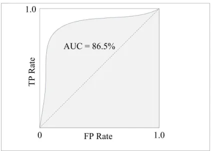
Area Under Curve (AUC)
While the ROC curve is a good visual aid in recognizing the performance of a given algorithm, a numeric value is sometimes needed for comparative purposes. The simplest way of calculating a value for the ROC is to measure the Area Under the ROC Curve (AUC) (Bradley, 1997; Zweig & Campbell, 1993). Since the ROC is plotted inside a unit square, the AUC’s value will always be between 0 and 1 (Figure 7).
Figure 7. Area Under Receiver Operating Characteristic Curve (AUC)
Graphing an ROC of random guesses will produce a straight line from 0, 0 to 1, 1 and an AUC of 0.5. Based on this, any good classifier should always have an AUC value greater than 0.5.
Based on their empirical studies, which compared the binary classification results of Decision Trees, Naive Bayes, and SVM across 13 distinct data sets, Huang and Ling (2005) concluded that researchers should use AUC evaluation as a performance measure
instead of accuracy when comparing learning algorithms applied to real-world data sets. This recommendation was based on their studies showing that AUC is a statistically consistent and more discriminating performance measure than accuracy. They also showed that by using the AUC evaluation to measure profits, a real-world concern, could be easier optimized.
Chapter 3
Methodology
Introduction
This study is a comparative analysis of feature selection methods on classification systems in a real domain setting. As with any data mining exercise, before the data are mined, several key steps need to be performed (Fayyad et al., 1996). These steps, referred to as the preprocessing stage, will account for dealing with missing values, balancing data, discretizing or normalizing attributes depending on which algorithm is used, and finally minimizing the dimensionality of the data set by reducing the number of features with different feature selection methods.
Data Mining Process
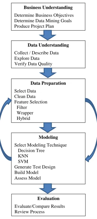
The data mining framework followed in this study was the Cross-Industry Standard Process for Data Mining (CRISP-DM), a non-proprietary hierarchical process model designed by practitioners from different domains (Shearer, 2000). The CRISP-DM framework breaks down the data mining process into six phases:
1) Understanding the business process and determining the ultimate data mining goals 2) Identifying, collecting, and understanding key data sources
3) Preparing data for data mining
4) Selecting which modeling technique to use
5) Evaluating and comparing results of different models against the initial goals
One distinctive feature of this framework is that it is more an iterative process than a straight flow design. Practitioners are encouraged to improve results by iterating through the data preparation process and model selection and use.
This researched used this framework and provided a structured way to conduct the experiments used in this comparative study. Therefore, it improved the validity and reliability of the final results.
Figure 8. Framework Used in this Research
Business Understanding Determine Business Objectives Determine Data Mining Goals Produce Project Plan
Data Understanding Collect / Describe Data Explore Data
Verify Data Quality
Data Preparation Select Data Clean Data Feature Selection Filter Wrapper Hybrid Modeling Select Modeling Technique Decision Tree
KNN SVM
Generate Test Design Build Model
Assess Model
Evaluation Evaluate/Compare Results Review Process
Data
We used two data sets for this analysis. The first data set to be analyzed was a vehicle service and sales data set that contains information about vehicle services performed and vehicle sales at over 200 auto dealerships. This data set contained thousands of records and thousands of attributes. The goal of this study was to determine the best performing feature selection method and classification algorithm combination that would help automotive dealerships determine if a particular vehicle owner would purchase a new vehicle based on service histories. The second data set was selected from the University of California, Irvine (UCI) Machine Learning Repository (Lichman, 2013) to compare results of our testing against other domains.
Data Acquisition
The data in the vehicle service and sales data set comes from the dealerships’ Dealer Management System (DMS) (Appendix A). Data was captured from both the service and sales departments. During a service visit, the vehicle’s owner information, vehicle
identification number (VIN), and service detail are recorded in the system. Similarly, on the sales side, customer’s information and vehicle information are saved into the system after every sale. At the end of each day all transactional data is transferred to a data warehouse server running Postgres SQL. The data is then extracted, transformed, and loaded into SQL Server using a SQL Server Integration Services (SSIS) ETL process (Figure 9).
The data set used in this study was extracted from the following 4 tables:
1. Customer 2. VehicleSales 3. ServiceSalesClosed 4. ServiceSalesDetail
A class label field was added to denote the purchase of a vehicle, new or used, after service was performed. The extraction process will join the data in these relational tables to produce a flat file in a format that the WEKA (Waikato Environment for Knowledge Analysis) (Witten et al., 2011) workbench recognizes. Refer to Appendixes A and B for complete list of attributes and data types.
Figure 9 . Da ta A cquisi ti on F low
Data Pre-Processing
Before running any classification algorithms on the data, the data must first be cleaned and transformed in what is called a pre-processing stage. During this pre-processing stage, several processes take place, including evaluating missing values, eliminating noisy data such as outliers, normalizing, and balancing unbalanced data.
Missing Values
Real world data generally contains missing values. One way of dealing with missing values is to omit the entire record which contains the missing value, a method called Case Deletion. However, Shmueli, Patel, and Bruce (2011) noted that if a data set with 30 variables misses 5% of the values (spread randomly throughout attributes and records), one would have to omit approximately 80% of the records from the data set. Instead of removing the records with missing values, different data imputation algorithms have been studied and compared. Among these methods are Median Imputation, K-NN Imputation, and Mean Imputation (Acuna & Rodriguez, 2004). Median Imputation, as its name implies, replaces the missing values in the record with the median value of that attribute taken across the data set. The K-NN method uses the K-NN model to insert values into the data set. Records with missing values are grouped with other records with similar characteristics which in turn provide a value for the missing attribute. Finally, the Mean Imputation method replaces the missing value with the mean or mode, depending on the attribute type, based on the other values in the data set. Farhangar, Kurgan, and Dy (2008) argued that mean imputation was less effective than newer methods, such as those based on Naives-Bayes methods, only when the missing data percentage in the data set surpassed 40%. They also concluded, like others (Acuna & Rodriguez, 2004), that any
imputation method was better than none. In addition, they reported that different imputation methods affected the accuracy classification algorithms differently.
In this study, we used the mean imputation method to populate our missing values. This decision was based on the percentage of missing values in our data set (< 20%) and its overall effectiveness in improving the accuracy of classification algorithms. The pseudo code for replacing the missing values is shown in Algorithm 1:
Algorithm 1 Mean Imputation Method
Let D = {A1, A2, A3,… An}
where D is the data set with missing values, Ai is the ith attribute column of D with missing value(s), and n is the number of attributes
For each missing attribute in 𝐴𝑖 {
If numeric, impute the mean value of the attribute in class
If nominal (i.e. good, fair, bad), impute the mode value of the attribute in class
}
Imbalanced Data
The problem of imbalanced data classification is seen when the number of elements in one class is much smaller than the number of elements in the other class (Gu, Cai, Zhu & Huang, 2008). If they are left untouched, most machine learning algorithms would predict the most common class in these problems (Drummond & Holte, 2005). Simple queries on our data set had shown us that the data set was imbalanced in respect to the
class label which we were working on. The majority of our records used in this research, 90%, fall into the “Did not buy vehicle” class as opposed to the “Bought a vehicle” class. Processing the data without changes may result in over fitting or under performance of our classifying algorithms. If the data set is small, we could rely on algorithms to synthetically create records to better balance the data. These algorithms, such as
Synthetic Minority Oversampling Technique (SMOTE) filter (Chawla, Bowyer, Hall, & Kegelmeyer, 2002), do just that. Since our main data set consisted of thousands of records we implemented a random undersampling (RUS) to balance our data. RUS removes records randomly until a specified balance (50:50 ratio in our case) is achieved. For instance, if a data set consists of 100,000 records in which 10% belong to the positive class that would leave 90,000 records belonging to the negative class. Undersampling this data set to achieve a 50:50 class ratio would remove 80,000 records and leave us 10,000 records in the positive class and 10,000 records in the negative class. While this method has been argued to remove important data from the classification analysis in small data sets (Seiffert, Khoshgoftaar, Van Hulse, & Napolitano, 2010) it is effective in larger ones (Lopez, Fernandez, Garcia, Palade, & Herrera, 2013). The pseudo code for RUS is shown in Algorithm 2:
Algorithm 2 Random Undersampling Method
1: Determine minimum/majority class ratio desired (i.e. 50:50 ratio) 2: Calculate number of tuples N in majority class that need to be removed
3: Select random tuples in majority class using a structured query
language statement such as: SELECT TOP N FROM
tblDealerData ORDER BY NEWID() 4: Save new data set
This sampling occurred before applying the classifier algorithms in WEKA.
Data Normalization
Some algorithms, such as Support Vector Machines and K-NN, may require that the data be normalized to increase the efficacy as well as efficiency of the algorithm. The normalization will prevent any variation in distance measures where the data may not been normalized. A prime example is that data values from different attributes are on a completely different scale, i.e. age and income. Normalizing the attribute will place all attribute within a similar range, usually [0, 1].
In this study we use a feature scaling normalization method to transform the values, using the following formula:
𝛿 = 𝑑 − 𝑑𝑚𝑖𝑛 𝑑𝑚𝑎𝑥 − 𝑑𝑚𝑖𝑛
where δ is our normalized value, 𝑑 is our original value, 𝑑max is maximum value in range, and 𝑑min is minimum value in range.
Data Discretization
Discretization is the process of converting continuous variables into nominal ones. Studies have shown that discretization makes learning algorithms more accurate and faster (Dougherty, Kohavi, & Sahami, 1995). The process can be done manually or by predefining thresholds on which to divide the data. Some learning algorithms may require data to be discretized. An example is the C4.5 decision tree. This tree algorithm does not support multi-way splits on numeric attributes. One way to simulate this is to discretize the attribute into buckets which can in turn be used by the tree.
Feature Selection
Part of this study was to compare the performance of classifiers based on the features selected. By omitting attributes that do not contribute to the efficacy as well as efficiency of the algorithm, we reduced the dimensionality of our data set and improved the
processing performance. Tests were conducted on the following feature selection categories:
Filters: Attributes were ranked and chosen independently to classifier algorithm to be used.
Wrappers: Attributes were selected taking the classification algorithm into account. Hybrid: Attributes were first selected using a filter method then a wrapper method.
Filters
The three filter methods we used in our study were:
1. Information Gain
2. Correlation-based Feature Selection (CFS) 3. Relief-F
These feature selection methods were chosen based on their differing approach in identifying key features.
Information Gain
The information gain filter (Quinlan, 1987) measures the attribute’s information gain with respect to the class. We began calculating our information gain by calculating the entropy for our class. Entropy was defined as follows (Shannon, 1948):
𝐼𝑛𝑓𝑜(𝐷) = − ∑ 𝑝𝑖log2(𝑝𝑖) 𝑚
𝑖=1
Where 𝐷 is our data sample, 𝑝𝑖 is the proportion of 𝐷 in respect to class 𝐶𝑖 and can be estimated as |𝐶𝑖,𝐷|
|𝐷| , and 𝑚 is the number of possible outcomes. The extreme entropy values
for 𝐼𝑛𝑓𝑜(𝐷)𝑚𝑎𝑥 are 1 (totally random) and the minimum is 0 (perfectly classified). 𝐼𝑛𝑓𝑜(𝐷) is the information needed to classify a tuple in D, also known as the entropy of
D.
The next step in calculating the information gain is to calculate the expected