Asset Return Prediction via Machine Learning

https://www.scirp.org/journal/jmf ISSN Online: 2162-2442

ISSN Print: 2162-2434

DOI: 10.4236/jmf.2019.94035 Oct. 30, 2019 691 Journal of Mathematical Finance

Asset Return Prediction via Machine Learning

Liangliang Zhang

NatWest Markets Securities, Ltd., Stamford, CT, USA

Abstract

In this paper, we provide insights on the prediction of asset returns via novel machine learning methodologies. Machine learning clustering-enhanced clas-sification and regression techniques to predict future asset return movements are proposed and compared. Numerical experiments show good applicability of the methodologies and backtesting unveils superior results in China A-shares markets.

Keywords

Clustering, Classification, Regression, Unsupervised Learning, Supervised Learning, Deep Neural Networks, Machine Learning, Asset Returns, Prediction, Investment Strategies, Universal Approximation Theorem

1. Introduction

Predicting asset returns is of central importance for empirical, theoretical and practical considerations. Essentially, prediction is the computation of the ortho-gonal projection of future asset returns, i.e., asset price movements, often mod-eled as stochastic processes, onto the information structure that we observe to-day. Described in mathematical language, prediction involves the computation of conditional expected asset returns.

From an empirical point of view, [1] proposes to decompose asset returns with respect to the underlying risk factors. More description can be found in [2]. The approach is, in principle, the same as relative pricing of financial derivatives, where the underlying risk factors are taken as primitives, modeled econometri-cally and the derivatives prices, i.e., the conditional expected discounted future cash flows, are expressed as a functional of them.

In this paper, we propose new methodologies to compute the conditional ex-pected asset returns under the risk-decomposition framework of [1]. We use non-linear functions to model the dependency of expected asset returns on risk factors and the nonlinearity is recovered from the market data in a model-free

How to cite this paper: Zhang, L.L. (2019) Asset Return Prediction via Machine Learn-ing. Journal of Mathematical Finance, 9, 691-697.

https://doi.org/10.4236/jmf.2019.94035

Received: October 6, 2019 Accepted: October 27, 2019 Published: October 30, 2019

Copyright © 2019 by author(s) and Scientific Research Publishing Inc. This work is licensed under the Creative Commons Attribution International License (CC BY 4.0).

DOI: 10.4236/jmf.2019.94035 692 Journal of Mathematical Finance manner. [3] runs a comparison of different machine learning methods on a monthly frequency in US equity market. [4] extends the analysis to fixed income markets. In [5], the authors recover the stochastic discount factor, project it onto the asset span and obtain the optimal weights considering the no-arbitrage con-straints. In all the references, the authors use a brute-force supervised learning approach to predict the asset returns as a regression problem. In this paper, we factor in the clustering techniques to compute conditional expected asset returns, first proposed in a derivative pricing setting in [6] to evaluate the conditional expectation at each point of time, expressed as function of risk factors. The me-thod utilizes non-supervised learning techniques, such as k-means clustering, to partition the factor space and in each of the sub-spaces, a simple functional form is used to approximate the non-linear relationship between the future asset re-turns and current values of underlying risk factors.

The contribution of this paper is three-folds. First, methodologically speaking, we combine unsupervised learning and supervised learning tech-niques to enhance the computation efficiency for regression and classification problems. Second, under our framework, machine learning techniques and clas-sical function approximation methodologies jointly deliver high-performance methods. This helps because, under limited computational resources, we can use as many past data as possible to train the model and meantime enjoy a fast-computational speed. Third, in terms of prediction, we propose to measure the expected absolute returns and the signs of the future price movements sepa-rately to increase the forecasting accuracy. Moreover, new stock selection criteria are proposed. This methodology enables us to use a larger number of factors and past data than the artificial neural network approach and meanwhile achieving a faster computational speed. Empirical studies in China A-share markets reveal superior results.

The organization of this paper is as follows. Section 2 describes the proposed techniques. Section 3 discusses backtesting methodologies and the results and Section 4 concludes. All the theoretical justifications can be found in the Ap-pendix.

2. The Prediction Methodology

In this section, we introduce the main methodologies of this paper. We show that both the currently used machine learning regression and classification problems can be embedded into our theoretical framework as special cases1_.

Then, we show that we can, instead of predicting asset returns in a brute force manner, enhance the prediction precision by separating the prediction of magnitude of the asset price changes with the directions.

2.1. Clustering-Based Regression

Let us first assume that the conditional expected asset returns can be expressed 1_{That is, when the number of clusters is 1, our method degenerates to the brute-force machine}

DOI: 10.4236/jmf.2019.94035 693 Journal of Mathematical Finance as continuous functions of risk factor values. The case with discontinuous func-tions is analogous with mollifiers. According to the definition of a continuous function, if its argument values are sufficiently close, then the dependent varia-ble values are also very close. If we further assume first order differentiation of the target function, it can be shown that, in a small region of the domain of the continuous function, we can approximate it well with linear functions. This ob-servation inspires us to use a clustering-based approach to enhance the classifi-cation or regression prediction for asset returns.

Suppose that the risk factors are denoted by an r-dimensional vector Xt. The

target function is ϕ. We are trying to compute ϕ

(

)

[

]

that at time t, the state space of the risk factor Xt is Dt. In what follows, we are

seeking a partition of this state space, denoted by

{ }

= such that in each of

the subspace k t

U , we use a linear function ϕk

(

)

(

) (

)

to approximate ϕ. The rigorous mathematical justifications of this approach are given in the Appendix.

The steps are as following. Given m assets, whose rate of return processes are denoted by

{ }

t _i R

= , suppose that we want to consider T periods of data.

Therefore, there are m T× observations in total for the r-dimensional factors. Partition, using MiniBatchKMeans function in Python, the m T× observa-tions into K clusters. In each of the cluster, use a simple neural network or just a linear regression model to fit the data via equation

(

) (

)

1 k , , , , , ,

t t

i

t t h _{X U} t

E R_{+ ∈}  =a t h i k +b t h i k X

  . Then, for each new observation

t h

X₊ , we first use predict function in python to decide which cluster it belongs to,

then use equation 2 1 k

(

) (

)

t t

i

t t h _{X U} t h

E R_{+ ∈}  =a t h i k +b t h i k X₊

  to compute

the expected return.

2.2. Clustering-Based Classification

Taking a two-category logistic regression-based classification as an example, we know that a classification problem is essentially a regression one. Therefore, we can use the clustering-based method introduced in Section Clustering-Based Regression to run the regression and conduct the classification. Multi-category classification problems are analogous.

3. Empirical Study

In this empirical study, we use two sets of machine learning architectures, which will be documented below.

3.1.1. Forecasting Magnitude and Directions of Asset Price Movements via Deep Learning

DOI: 10.4236/jmf.2019.94035 694 Journal of Mathematical Finance

p

c . If c_u−c_l is large, the point estimate is useless since it is indicated that the

forecasting errors might be large, and the realized values can deviate from the point estimate cp. We hope to propose a method to narrow the confidence

in-terval and therefore make the point estimate more reliable. The key is to separate the estimation of the magnitude and sign of the future asset price returns. De-note by Rt the asset return at time t. Then, we will try to take two steps. The

first step is to compute Et Rt h+ ,

2

t t h

E _R₊ _ and therefore VAR_t_R_{t h+} _. The

second step is to use a two-category classification algorithm to label 0 if 0

t h

R₊ ≤ and 1 otherwise. If the probability associated with the classification of

label 0 is larger than a threshold α , then we categorize that the future return will be negative. On the other hand, if the probability of label 1 is larger than α_,

then we categorize that the future return will be positive. After we determine the sign of the future expected returns, we can use the result from the first step, i.e., the estimates of EtRt h+  as the magnitude of the expected returns. If Rt h+ is

estimated to be positive and EtRt h+ −qα VARtRt h+ >θt or Rt h+ is

esti-mated to be negative and EtRt h+ +qα VARtRt h+ < −θt, then we go long

or short the asset accordingly, where q_α is an appropriate quantile and θ_t is

the return deduction because of the transaction cost. The regression and classi-fication can, of course, be done via deep learning techniques. To reduce computational resource requirement, both the regression and classification can be done by introducing the clustering method described above. We will mainly test this methodology with China A shares.

3.1.2. Clustering-Based Regression

This method is a direct application of the clustering-based regression method introduced in Section 2.1. For each asset, we forecast E Rt

[

]

2

t t h

E _R₊ _ and

t t h

VAR _R₊ _. Decide on a percentage α and compute the information ratio

[

]

t t h

t t h

E R

VAR R

+

+

 

  . Rank the information ratio in the cross-section of asset universe, long the top α percent and short the bottom α percent. However, for this methodology, we try not only to predict the forward 1 period return for each asset, but the entire forward n period-curve as well. This means at each moment in time t, we will predict

{

[

]

}

t t ih _i

E R_{+ =} . Then, long at bottom and sell at peak of

the curve. Of course, we can consider the forecasting accuracy by looking at the confidence intervals. That is, whenever the accuracy exceeds some predeter-mined thresholds, we can view the forecasted values as valid. We will test this method using China A-shares.

3.1.3. Choice of Pricing Factors

DOI: 10.4236/jmf.2019.94035 695 Journal of Mathematical Finance 3.2. The Data

The China A-share market data, including the stocks traded in Shanghai and Shenzhen stock exchanges, are downloaded from Wind terminal. Time ranges from 2008-1-2 to 2019-5-23.

3.3. Backtesting

3.3.1. Strategy 1 Performance

For Strategy 1, we use a rolling window of 250 days to compute the factor values. In order to train the clustering and regression model, we use a panel data of past rolling 100 days. To compute the regression model, we use a clustering-based approach with 100 clusters in all and we choose the five clusters with top per-formance to trade. This strategy is long only. Transaction cost and slippage are assumed to be unilateral 0.15%. Table 1 and Figure 1 document the perfor-mance for Strategy 1.

3.3.2. Strategy 2 Performance

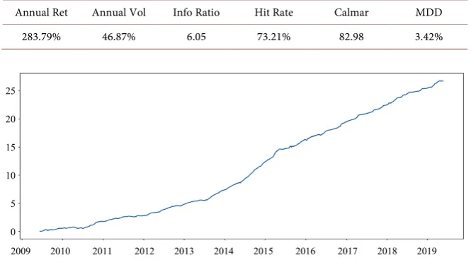
For Strategy 2, we use a rolling window of 250 days to compute the factor values. In order to train the regression model, we use panel data of past rolling 100 days. To compute the regression model, we use a clustering-based approach with 100 clusters in all and we choose the five clusters with top performance to trade. This strategy is long-short. Table 2 documents the performance for Strategy 2.

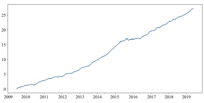
The NAV plot of a long-only strategy based on the methodology in Section 3.1.2 is shown in Figure 2. Transaction cost and slippage are assumed to be un-ilateral 0.15%.

Table 1. Performance for strategy 1.

Annual Ret Annual Vol Info Ratio Hit Rate Calmar MDD

203.56% 36.94% 5.49 72.47% 69.47 2.93%

Table 2. Performance for strategy 2.

Annual Ret Annual Vol Info Ratio Hit Rate Calmar MDD

283.79% 46.87% 6.05 73.21% 82.98 3.42%

DOI: 10.4236/jmf.2019.94035 696 Journal of Mathematical Finance

Figure 2. NAV plot-long only for china a-share market.

4. Conclusion

In this paper, we propose a clustering-based methodology to compute the ex-pected asset returns and create trading strategies based on it. Numerical results show superior performance in China A-Share markets. Future research includes applying the proposed approach in LSTM or reinforcement learning contexts.

Conflicts of Interest

The author declares no conflicts of interest regarding the publication of this paper.

References

[1] Ang, A. (2013) Factor Investing. https://doi.org/10.2139/ssrn.2277397

[2] Homescu, C. (2015) Better Investing through Factors, Regimes and Sensitivity Analysis. https://doi.org/10.2139/ssrn.2557236

[3] Gu, S., Kelly, B. and Xiu, D. (2018) Empirical Asset Pricing via Machine Learning.

https://doi.org/10.3386/w25398

[4] Bianchi, D., Buchner, M. and Tamoni, A. (2018) Bond Risk Premia with Machine Learning. https://doi.org/10.2139/ssrn.3232721

[5] Chen, L., Pelger, M. and Zhu, J. (2019) Deep Learning in Asset Pricing.

https://doi.org/10.2139/ssrn.3350138

DOI: 10.4236/jmf.2019.94035 697 Journal of Mathematical Finance

Appendix

We will only consider the case where the functions are continuously defined on a compact domain of _Rr. The extension to general functions which are defined

in r

R is straightforward with mollifiers and the assumption that the

distribu-tions of asset returns are exponentially decaying at tails. We first need the fol-lowing assumption.

Assumption A.1 (On Function Representation). For any asset return R, we have ϕ

(

)

[

]

ex-pressed as functions of state variables.

Lemma A.2 (On Lead-Lag Regression). Suppose that Φ is an appropriate function space. Then, we have

( )

(

)

(

)

(

)

arg minϕ∈ΦE_ψ X_T −ϕ t X, _t _=arg minϕ∈ΦE_ϕ t X, _t −ϕ t X, _t _

where *

(

)

( )

, _{t t T}

t X E X

ϕ = _ψ _.

Proof of Lemma A.2. The proof of this lemma follows from Theorem 8 of [6]. Theorem A.3 (On Polynomial Regression). Assume that ψ _{is a}

conti-nuous function defined on a compact domain U,

{ }

= is a partition of

do-main U and

(

)

_{( )}

( )

( )

,

ˆ , arg min _k

J J t

k J t Xt _{p P U} E XT pJ Xt

ϕ = _∈ _ψ − _

where

( )

J t

P U is the space of all polynomials, whose coefficients depend on

time t and T, with degree less or equal to J. Then, we have

(

)

_{( )}

(

)

1 ,

max 0

1 ˆ

, lim k , 1 k

t t k K t

K

t _{d U} k J t _{X U}

k

t X t X

ϕ ϕ

≤ ≤ → ₌ ∈

=

∑

here distance d U

( )

Proof of Theorem A.3. The proof of this theorem follows from Lemma A.1, Theorem 23 of [6] and Cauchy-Schwarz inequality.