Non-perturbative Calculation of Molecular Magnetic Properties within Current-Density Functional Theory
E. I. Tellgren,1,a) A. M. Teale,2, 1,b) J. W. Furness,2 K. K. Lange,1 U. Ekstr¨om,1 and T. Helgaker1
1)Centre for Theoretical and Computational Chemistry, Department of Chemistry,
University of Oslo, P.O. Box 1033 Blindern, N-0315 Oslo,
Norway
2)School of Chemistry, University of Nottingham, University Park, Nottingham,
NG7 2RD, UK
Abstract
We present a novel implementation of Kohn–Sham density-functional theory
uti-lizing London atomic orbitals as basis functions. External magnetic fields are treated
non-perturbatively, which enables the study of both magnetic response properties and
the effects of strong fields, using either standard density functionals or current-density
functionals—the implementation is the first fully self-consistent implementation of
the latter for molecules. Pilot applications are presented for the finite-field
calcu-lation of molecular magnetizabilities, hypermagnetizabilities and nuclear magnetic
resonance shielding constants, focusing on the impact of current-density functionals
on the accuracy of the results. Existing current-density functionals based on the
gauge-invariant vorticity are tested and found to be sensitive to numerical details
of their implementation. Furthermore, when appropriately regularized, the resulting
magnetic properties show no improvement over standard density-functional results.
An advantage of the present implementation is the ability to apply density-functional
theory to molecules in very strong magnetic fields, where the perturbative approach
breaks down. Comparison with high accuracy full-configuration-interaction results
shows that the inadequacies of current-density approximations are exacerbated with
increasing magnetic field strength. Standard density-functionals remain well behaved
but fail to deliver high accuracy. The need for improved current-dependent
density-functionals, and how they may be tested using the presented implementation, is
discussed in light of our findings.
PACS numbers: Valid PACS appear here
I. INTRODUCTION
Accurate and efficient calculation of magnetic properties is an important challenge for
quantum-chemical methods. The effects of the magnetic fields available in laboratory
exper-iments tend to be very weak compared with the natural energy scale for a small molecule,
and so the dominant approach to the calculation of molecular magnetic properties has relied
on the use of perturbation theory.1,2 Both static and dynamic properties may be computed
within this framework, although equations and implementations for high-order properties
rapidly become unwieldy.
Recent work has developed an alternative, non-perturbative, gauge-origin-invariant
ap-proach to study molecules in magnetic fields,3,4 without recourse to perturbation theory.
Apart from offering a simple and convenient way to estimate static response quantities, this
approach enables the study of molecules subject to very strong magnetic fields, for which
a perturbation expansion converges very slowly, if at all.4–6 In both perturbative and
non-perturbative approaches, London atomic orbitals provide an efficient means of accelerating
basis-set convergence by building part of the magnetic response and some gauge degrees
of freedom into the basis functions. In particular, the use of London orbitals makes the
calculations invariant to the choice of gauge origin for uniform magnetic fields.
While previous work was concerned with the Hartree–Fock3 and
full-configuration-interaction (FCI)6 levels of theory, the present work explores the use of Kohn–Sham
density-functional theory (KS-DFT) in magnetic fields. The standard formulation of KS-DFT is not
rigorously valid in the presence of an external magnetic field. Instead, the theory needs to be
generalized and some additional ingredient besides the charge density needs to be included
in the universal exchange-correlation functional—either the magnetic field7 or the current
density.8 We focus here on Vignale and Rasolt’s formulation of current-density functional
theory (CDFT), in which this extra ingredient is the paramagnetic current density.8–10
In practice, nearly all applications of DFT to molecular magnetic properties are
per-formed with standard, density-dependent exchange–correlation functionals, often developed
primarily for energetics in the absence of magnetic fields. As recently documented by
com-parison with high-accuracy coupled-cluster results for magnetizabilities and rotational g
tensors11 and for nuclear shielding and spin–rotation constants12, the accuracy achieved by
Kohn–Sham results are no better than the Hartree–Fock results and never better than the
CCSD results. It has been suggested that the use of CDFT may lead to improved results.
In this paper, we present an implementation of (C)DFT using London atomic orbitals. We
commence in Section II by presenting the theoretical modifications to KS-DFT necessary
in the presence of a magnetic field, focusing on the Vignale–Rasolt (VR) formulation of
CDFT and the associated vorticity-dependent exchange–correlation functionals available in
the literature. In Section III, we present our implementation of a (C)DFT module in the
londonprogram, capable of performing both standard DFT and CDFT calculations in the
presence of magnetic fields. Results using CDFT are presented in Section IV for magnetic
properties typically accessible by response theory. Comparisons of these results with recent
benchmark data and those from standard DFT calculations allow us to assess the quality of
the different CDFT functionals. In Section V, we extend our study to field strengths where
response theory is no longer applicable; in this regime, the results are compared with those
obtained from FCI calculations. Finally, in Section VI, we make some concluding remarks
and discuss directions for future work.
II. THEORY
In the present section, we first consider the Vignale–Rasolt formulation of CDFT in
Section II A; next, we consider the VRG functional and its parameterizations in Section II B.
A. The Vignale–Rasolt universal CDFT functional
In the presence of a magnetic field, the non-relativistic electronic Hamiltonian takes the
form (atomic units)
ˆ
H[v,A] = 1 2
N
X
k=1
(ˆpk+A(rk))2 + N
X
k=1
v(rk) + 1 2
N
X
k6=l 1
rkl
, (1)
where N is the number of electrons, ˆpk is the canonical-momentum operator of electron
k, v(r) is the external scalar potential at position r, and the magnetic vector potential
ground-state energy may then be expressed as follows,8
E[v,A] = inf ψ hψ|
ˆ
H[v,A]|ψi
= inf ρ,jp
F[ρ,jp] + Z
(ρv+ 1 2ρA
2+j
p·A) dr
, (2)
where ρ is the electron density, jp is the paramagnetic current density, and F[ρ,jp] is the
Vignale–Rasolt constrained-search universal current-density functional:
F[ρ,jp] = inf
ψ7→ρ,jp
hψ|Hˆ[0,0]|ψi. (3)
In Kohn–Sham theory, this functional may be decomposed further into a Kohn–Sham
non-interacting kinetic-energy term Ts[ρ,jp], a Hartree term J[ρ], and an exchange–correlation
term Fxc[ρ,jp]:
F[ρ,jp] =Ts[ρ,jp] +J[ρ] +Fxc[ρ,jp]. (4)
From gauge-invariance considerations, Vignale and Rasolt argued that the exchange–
correlation energy depends only on jp through the gauge-invariant vorticity,
ν(r) =∇ × jp(r) ρ(r)
= ρ(r)∇×jp(r)−∇ρ(r)×jp(r)
ρ(r)2 . (5)
In the expressions given above, the spin degrees of freedom and the spin-Zeeman term
have been neglected. The literature contains slightly different formalisms for taking these
into account. In particular, F and Fxc have been considered functionals of the following
variables:
1. the total densityρ, the spin densitym, and the total paramagnetic current density jp,
2. the total densityρand the total paramagnetic current–spin densityjm=jp+∇×m,13
3. the fully spin-resolved densities ρ↑ and ρ↓ and the paramagnetic current densities jp;↑
and jp;↓.9
The choice between spin-resolved or total densities matters in particular for the vorticity,
which is not additive with respect to spins, νtot 6=ν↑+ν↓ and which vanishes identically for
densities arising from a single natural orbital (or Kohn–Sham orbital). Hence, it is possible
present work, we apply existing approximate functionals to closed-shell systems, for which
these distinctions do not matter. We therefore suppress spin indices in the following.
The fact that vorticities arising from a single orbital vanish identically raises the question
as to which paramagnetic densities (ρ,jp) can be represented by a Kohn–Sham
ground-state wave function. Clearly, a closed-shell two-electron system with a nonzero total
vor-ticity is neither non-interacting v-representable nor N-representable by a Kohn–Sham
sys-tem. Moreover, an open-shell two-electron system may feature non-vanishing spin
vor-ticities, which also cannot be represented by a Kohn–Sham system; see also Taut et al.
for a discussion of non-interacting v-representability in two-electron systems.14 For N ≥ 4
electrons, a recent result shows that all paramagnetic densities satisfying mild regularity
conditions are non-interacting N-representable.15 Depending on how the question of
non-interacting N-representability is resolved for few-particle systems and how non-interacting
v-representability is resolved forN ≥3, a rigorous approach to CDFT may require extended
(ensemble) Kohn–Sham theory and the use of methods for determining fractional
occupa-tion numbers.16–19It has recently been proved that essentially any density and paramagnetic
current density (subject only to the minimal regularity condition that a von Weizs¨acker-like
bound on the kinetic energy is locally integrable) are N-representable in extended Kohn–
Sham CDFT.20
B. The VRG exchange–correlation functional
Compared with the very large number of DFT exchange–correlation functionals, there
exist only a handful of specific CDFT functionals. Some of these are based on the vorticity
expansion and take the general form
FVRG[ρ,ν] = Z
g(ρ(r)) |ν(r)|2dr, (6)
where approximations to g(ρ) have been established from models of the uniform electron
gas. Indeed, such a functional form was considered by Vignale and Rasolt already in Ref. 8
and subsequently fitted to reference values computed with the random-phase approximation
(RPA) by Vignale, Rasolt, and Geldart (VRG) in Ref. 21
This original parameterization has been revisited several times—specifically, re-parameterizations
Capelle (OMC),24 by Tao and Perdew (TP),25 and by Tao and Vignale (TV).26
Addition-ally, Higuchi and Higuchi (HH)27,28 have constructed an approximate exchange–correlation
functional designed to satisfy exact conditions derived from scaling relations for the CDFT
exchange and correlation energies.
For molecules, it is essential that the parameterization of the VRG functional has a
sensible low-density limit. However, in the above parameterizations, fitting reference data
for g(ρ) were available only for Wigner–Seitz radii in the range 0 < rs ≤ 10 (VRG, LHC,
OMC, TP) and in the range 0 < rs ≤ 20 (TV). The low-density limit is consequently
underdetermined by the reference data.
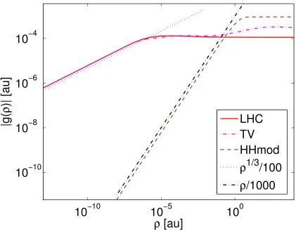
The low-density behaviour of the different parametrizations is shown in Fig.1.
Impor-tantly, the original VRG form and the OMC re-parametrization do not tend to zero in the
low-density limit, making them ill-suited for molecular applications. By contrast, the LHC,
TP, and TV re-parametrizations do tend to zero, albeit slowly—for sufficiently small ρ, we
find that
gLHC(ρ)≈gTP(ρ)≈gTV(ρ)∼ −ρ1/3. (7)
For the LHC and TV re-parameterizations, which result in everywhere negative functions
gLHC(ρ) andgTV(ρ), respectively, this decay behaviour is readily visualized in a log–log plot;
see Fig. 2 (the TP parametrization is not shown as it differs very little from TV on the scale
of the plot and the low-density asymptotes coincide).
Higuchi and Higuchi’s exchange functional HHx is constant: gHHx(ρ) = 2×3.76×10−4 a.u.
By adjusting this constant (i.e., setting ¯Dx =−C¯0 in the notation of Ref. 27), it is possible to
make their totalgHH(ρ) almost vanish for small densitiesρ10−30a.u; see Fig. 2. However,
the Higuchi–Higuchi correlation functional HHc has a singularity at ρ = 10−30a.u., so the approach to the low-density limit is interrupted by an infinite discontinuity. We denote the
modified Higuchi–Higuchi functional by HHmod.
Finally, we note that Zhu and Trickey29 compared vorticity-dependent functionals with
an exactly solvable model for a Hooke’s atom in a magnetic field, reporting that the vorticity
is a difficult quantity to work with. An alternative approach has been proposed by Becke,30
while a more elaborate version (relying on currents from individual Kohn–Sham orbitals)
was proposed by Pittalis et al.31 These functionals are based on the observation that a
gauge-invariant density can be formed from a combination of the Kohn–Sham
Kohn–Sham orbitals that give rise to the densities ρand jp, the quantity
e
τ(r) = 12X k
|∇φk(r)|2−
|jp(r)|2
2ρ(r) (8)
is gauge invariant.32The paramagnetic current can therefore be incorporated in an
exchange-correlation functional viaeτ. Exploration of this alternative is beyond the scope of the present
work.
III. IMPLEMENTATION
In our calculations, we consider a uniform magnetic field B, described by a cylindrical
vector potential
A(r) = 1
2B×(r−g), (9)
where g is the gauge origin. In exact calculations, with complete orbital basis sets, the
values of physical quantities are independent of the gauge origin (in fact, invariant to all
gauge transformations). For finite basis sets, gauge-origin invariance can be ensured by
employing London orbitals of the form
ωγ(r) =χγ(r) e−iA(Nγ)·r, (10)
where χγ(r) is a standard Gaussian-type basis function centred on Nγ and A(Nγ) is the
vector potential evaluated at the centre of the Gaussian. Effectively, the basis then becomes
a hybrid plane-wave/Gaussian basis for finite magnetic fields.3
The main modifications to the existing London Hartree–Fock code3 in order to enable
(C)DFT calculations are the implementation of a numerical integration scheme, the
evalua-tion of quantities such asρ(r),∇ρ(r), jp(r), andν(r) on the associated numerical grid and
the assembly of these components in the expressions for the exchange–correlation energies
and the functional derivatives required for their associated potentials.
For the molecular numerical integration, we construct a set of grid points and weights
using Becke’s space partitioning scheme with atomic size corrections,33 decomposing the
molecular integral into a sum of one-centre atom-like integrations. To eliminate crowding
of points close to nuclei, grid pruning is implemented using the approach outlined by
Mur-ray, Handy and Laming.34 For the radial part of these integrations, we employ the scheme
quadrature.36–41 We have tested our C++ implementation for standard density functionals
by comparing with the Dalton quantum chemistry program,42,43 in which similar Fortran
77 angular and radial implementations are available. Because of the slow decay of the
vorticity-dependent integrand in the present VRG parameterizations, we have used very
conservative screening criteria when processing points on the integration grid.
The evaluation ofρ(r),∇ρ(r),jp(r), andν(r) at the grid points is straightforward, given
the elements of the one-particle reduced density matrixDγζ and the values of basis functions
ωγ(r) and their gradients∇ωγ(r) at the grid points:
ρ(r) = X γζ
ωγ(r)Dγζ ωζ∗(r), (11)
∇ρ(r) = X γζ
ωγ(r)Dγζ ∇ω∗ζ(r) + c.c., (12)
jp(r) =
i 2
X
γζ
ωγ(r) Dγζ ∇ωζ∗(r) + c.c., (13)
where “c.c.” denotes the complex conjugate of the preceding expression. (Note that we work
with thenumberdensity and numbercurrent rather than theelectricaldensity andelectrical
current, the difference being a factor of −e in general, or−1 in atomic units.) Notably, the
curl ofjpcan be computed from the first-order functional derivatives of basis functions since
the second-order derivatives cancel:
∇×jp(r) = i X
γζ
Dγζ∇ωγ(r)×∇ωζ∗(r). (14)
At first glance, the right-hand side looks like an imaginary quantity; however, for a complex
vectorw, the cross-product iw×w∗ is real. A transformation to natural orbitals (or Kohn– Sham orbitals) thus makes it clear that the right-hand side is real.
The vorticity may be assembled from the above densities using the right-hand side of
Eq. (5) above. In practice, to guard against division by near-zero and the resulting loss of
precision, we prefer the regularized vorticity
ν(r) =
ρ(r)∇×jp(r)−∇ρ(r)×jp(r) p
4+ρ(r)4 , (15)
whereplays the role of a soft density cut-off. This regularization results in an underestimate
Once the required (C)DFT quantities have been assembled at the grid points, the
exchange–correlation energies and the derivatives required for construction of their
associ-ated Kohn–Sham matrix contributions can be calculassoci-ated. For the standard DFT
contribu-tions, we use the flexibleXCFunpackage,44 which uses automatic differentiation to provide
derivatives of the exchange–correlation energies from specified energy expressions. Once
these contributions have been evaluated, London constructs the associated Kohn–Sham
matrix elements.
For the CDFT contributions (which in the present work are added as corrections to
standard functionals), we have implemented the exchange–correlation energy and Kohn–
Sham matrix element constructions in the London code. For FVRG(LHC) and FVRG(TV),
which have everywhere negative integrands, the regularization of Eq. (15) is used and the
corresponding vorticity correction is therefore underestimated—at least when applied
non-self-consistently. For VRG parameterizations that decay asρ1/3 in the low-density limit, the
regularization in Eq. (15) yields a VRG integrand of the form
g(ρ)ν2 ∼ −ρ1/3|ρ∇×jp−∇ρ×jp|
2
4+ρ4 . (16)
Without regularization (i.e., with = 0), this decay may be numerically problematic—
in regions where the vorticity vanishes or is very small, numerical noise in the squared
factor would be amplified by a factor ρ−11/3. The need for appropriate regularization of the
vorticity has been noted in Ref. 45. The sensitivity of calculated properties to the choice of
the regularization parameters is investigated in Section IV.
IV. (C)DFT IN THE PERTURBATIVE REGIME
Over the last two decades, perturbative calculations of second-order properties such as
magnetizabilities and nuclear shielding constants have become routine in quantum chemistry,
also with London atomic orbitals. Properties that require higher-order responses such as
hypermagnetizabilities have received much less attention. Perturbative approaches have
been applied at the coupled-perturbed Hartree–Fock level using standard (non-London)
orbitals have been explored by Pagola et al.,46,47 while the finite-difference approach has
been explored by us at the Hartree–Fock level using London orbitals.3 However, we are not
treatment.
In this section, we present applications of CDFT to magnetizabilities, fourth-rank
hy-permagnetizabilities, and nuclear shielding constants. The implementation of molecular
properties is much simpler by finite-field techniques than that by perturbation techniques,
allowing us to assess readily the performance of a variety of CDFT functionals,
compar-ing their results with Hartree–Fock theory, the correspondcompar-ing DFT functionals and (where
available) accurate benchmark data.
We have performed calculations on a set of 27 molecules used in Ref. 12 at their
CCSD(T)/cc-pVTZ optimized geometries, namely, AlF, C3H4 (cyclopropene), FCCH, C2H4,
H2C2O (ketene), CH3F, CH4, CO, FCN, HCN, HCP, HF, LiH, LiF, NH3, N2, N2O, PN,
H4C2O (oxirane), OCFH, CH2O (formaldehyde), OCS, OF2, HOF, H2O, H2S, and SO2 (O3
has been excluded because of its multi-reference character). In all cases the aug-cc-pCVTZ
London atomic orbital basis set has been employed. The CDFT vorticity dependent
func-tionals were regularized with a hard cutoff on the Wigner–Seitz radius, rs, of 9.1055 a.u.
and a soft cutoff = 10−14 a.u., see Eq. (15). Experimentation revealed that results were
not particularly sensitive to the angular or radial grid parameters. The default parameters
were therefore used. For the Lebedev grid, the angular integration was specified to be
exact for spherical harmonics up to order 35; in the LMG radial integration, the accuracy
parameter specifying the upper limit of the error in the case of an atomic integration was
set to 10−13 a.u.
Even when employing the regularisation of Eq. (15) issues with SCF convergence were
still encountered for the VRG(LHC) parameterised CDFT corrections at some field strengths
when employing the standard direct-iteration-in-the-iterative-subspace (DIIS) approach.
In-terestingly, no such issues were encountered with the VRG(TP) parameterisation, for which
calculations on the full set of 27 molecules could be routinely performed at a range of field
strengths up to 1 a.u. This may reflect differences in the functiong(ρ) examined in Figures 1
and 2. In particular, the 8 molecules CH3F, HCN, HCP, H4C2O, CH2O, OCS, OF2 and SO2
could not be reliably converged using the VRG(LHC) parameterisation. To account for
this all plots and error analyses in the main manuscript refer to the remaining subset of
19 molecules. The full data set may be found in the supplementary material48, including
VRG(TP) based results for all 27 molecules. We emphasize that some regularization is
to similar numerical difficulties. We observe that these issues are, however, somewhat less
severe with the VRG(TP) parameterization than with VRG(LHC).
A. Molecular magnetizabilities and hypermagnetizabilities
Consider a uniform magnetic field B whose vector potential is given by Eq. (9).
Expand-ing the energy in orders of B, we obtain for a closed-shell system,
E(B) =E(0)− 1
2
X
αβ
χαβBαBβ
− 1
4!
X
αβγζ
XαβγζBαBβBγBζ+O(B6), (17)
where odd-order terms vanish. The magnetizability tensor χαβ and fourth-rank
hypermag-netizability tensorXαβγζ can be obtained by least-squares fitting of a polynomial to energies
E(Bα`) for a suitable discrete grid of a sample fields Bα`. We consider here only the
di-agonal tensor elements (which require less fitting data), using Bα` = `eα. It was found
that ` = 0.00,0.01, . . . ,0.03 a.u. in each Cartesian direction, α ∈ {x, y, z} provided
suf-ficient data to accurately determine molecular magnetizabilities and shielding constants;
the results reproducing those of the perturbative Dalton42,43 implementation to better
than 0.1×10⁻³⁰ JT−2 and 0.1 ppm, respectively, for standard density functionals. Careful
study of the convergence of hypermagnetizabilities revealed that higher field strengths were
required to obtain robust results and the grids used were supplemented with the points
`= 0.03,0.04, . . . ,0.1 a.u. in each Cartesian direction, making the calculations considerably
more expensive. The tensor elements were calculated by fitting 6th-order polynomials in
each cartesian direction.
In a previous benchmark study of magnetizabilities and g tensors calculated from
stan-dard DFT functionals, Lutnæset al.found that the standard DFT functionals (which neglect
the current dependence) in general give poorer results than does the Hartree–Fock model.11
Moreover, whereas the Hartree–Fock model (like the coupled-cluster models) on average
underestimates magnetizabilities, the LDA and GGA functionals overestimate the
magneti-zabilities. In Fig. 3, we have plotted the magnetizabilities obtained using the conventional
LDA, PBE, and KT3 functionals without current correction and with the VRG(LHC) and
same systems. We see the same trends as observed in Ref. 11, the LDA, PBE, and KT3
func-tionals overestimating the magnetizabilities and being less systematic than the Hartree–Fock
model.
Unfortunately, the addition of the VRG functional (with the LHC and TP
parameter-izations) does not improve the situation. For all three DFT functionals, the VRG(LHC)
correction increases the error in the magnetizabilities, increasing both mean errors and the
spread. The results are slightly better for the VRG(TP) functional but still poorer than
those obtained without the VRG correction. Clearly, the VRG-corrected functionals cannot
be recommended for the calculation of magnetizabilities. We note that Lee, Collwell and
Handy22 studied magnetizabilities for a few small systems in the context of CDFT using
a perturbative implementation. Many of the systems they considered are included in the
present work, however, a direct comparison is difficult because of the use of different basis
sets and the fact that the results of Ref. 22 are not gauge-origin invariant. The present
results may therefore be considered a more extensive benchmark addressing some of the
issues associated with these earlier calculations.
In Table I, we have listed the hypermagnetizabilities calculated at the Hartree–Fock, KT3,
and PBE levels of theory, all without VRG corrections; the corresponding VRG-corrected
results may be found in the supplementary material48. To our knowledge, these are the first
published Kohn–Sham hypermagnetizabilities.
We observe an overall qualitative agreement between the KT3 and PBE hypermagnetizabilities—
except for N2 and HFCO, the results agree on signs and relative magnitudes. As expected,
the agreement with the uncorrelated Hartree–Fock model is poorer, with more instances of
sign differences. However, without high-quality reference data (such as those provided by
coupled-cluster theory), it is difficult to assess properly the performance of the Hartree–Fock
and Kohn–Sham DFT models for hypermagnetizabilities.
We have carried out Kohn–Sham calculations of hypermagnetizabilities with the VRG
correction added; the results are included in the supplementary material48. In nearly all
cases, the VRG correction to the hypermagnetizability tensor elements is negative;
how-ever, in the absence of accurate reference data, it is difficult to judge the quality for the
CDFT results for the hypermagnetizabilities. Bearing in mind the poor performance of the
VRG correction for magnetizabilities, it is a safe assumption that the hypermagnetizability
B. Nuclear shielding constants
In a recent benchmark study of NMR shielding constants and spin–rotation constants,12
the accuracy achieved by Kohn–Sham calculations was found to be rather low. Although the
various DFT approximations improve slightly upon the Hartree–Fock theory results, none
of the DFT functionals provide an accuracy similar to that of CCSD or CCSD(T) theory;
moreover, the inclusion of vibrational corrections worsened the agreement with experimental
values. Regarding the different exchange–correlation functionals, a general improvement was
observed when going from LDA to GGA functionals, with further improvements observed
for hybrid functionals—in particular, in combination with an optimized-effective-potential
(OEP) approach. Interestingly, KS[CCSD] and KS[CCSD(T)] calculations, where the Kohn–
Sham system reproduces the CCSD and CCSD(T) densities, respectively, gave errors similar
to those of the OEP calculations. This suggested that the neglect of current dependence
may be a significant factor in determining the accuracy of these calculations.
To calculate NMR shielding constants non-perturbatively we consider the dependence of
the molecular electronic energyE(B,Mk) on the external magnetic field Band the nuclear
magnetic moment Mk of nucleus k represented by the vector potential,
Ak(r) =
µ0
4π
Mk×(r−K)
|r−K|3 =
µ0
4πMk×
1
∂K
1
|r−K|, (18)
where Kis the position of the nucleus. We obtain the Taylor expansion
E(B,Mk) = E(0,0) +
X
αβ
σk;αβBαMk;β+· · · (19)
where the nuclear shielding tensor is the leading-order mixed term in the expansion of the
energy,
σk;αβ =
∂2E(B,M
k)
∂Bα∂Mk;β
B=0,Mk=0
. (20)
The kinetic-energy operator in the Hamiltonian now becomes (atomic units) ˆπ2/2 = (ˆp+
A(r) +Ak(r))2/2. Exploiting the Hellmann–Feynman theorem, we compute the derivative
with respect to Mk analytically,
Ξk;β(B) =
∂E(B,Mk)
∂Mk;β
M
k=0
= eµ0 4πmαβγ
∂ ∂Kγ
hψ|
ˆ
where the braces denote the anti-commutator. The expectation value is similar to a nuclear
attraction integral, and may be evaluated using the McMurchie–Davidson scheme described
in previous work.3 The remaining differentiation may be performed directly by numerical
differentiation,
σk;αβ ≈
Ξk;β(eα)−Ξk;β(−eα)
2 =
Ξk;β(eα)
, (22)
or indirectly by polynomial fitting to computed Ξk;β(B) values as a function of B. The
fitting is simplified by the fact that only odd-orders ofB enter in the expansion of Ξk;β(B).
Before considering the benchmark calculations, we have in Fig. 4 plotted the VRG
cor-rections to the oxygen shielding constant in H2O against the integration cut-off parameter
ρcut-off(with hard and soft cut-offs) for the LHC, TP, and HHmod parameterizations ofg(ρ).
Substantial variations in the corrections are observed and no convergence is achieved with
reasonable cut-offs—in particular, for the LHC parameterization (with variations over about
60 ppm in the plot). The LDA- and BLYP-based VRG corrections are similar to each other
for cut-offs larger than about 10−5; for smaller cut-offs, the LDA-based corrections tend to
be larger than the BLYP-based corrections. Moreover, the differences between the
correc-tions obtained with hard and soft cut-offs are small compared with the differences observed
for different cut-off parameters.
The TP correction is much better behaved, with variations on the order of 3.5 ppm and
a consistent sign for the correction term. However, this variation and a lack of convergence
with respect to varying the cutoff parameters mean that it cannot be recommended for
practical use. The HHmod parameterisation shows a large variation with regularisation
parameters and so also cannot be recommended for practical use. However, it is interesting
that for the large cutoff values HHmod leads to a negative correction, which is opposite
in sign to the high cutoff value LHC and TP corrections. This difference may reflect the
qualitative difference in the functionsg(ρ) in Figures 1 and 2, in particular for large densities
gHHmod(ρ) is positive, whilst gLHC(ρ) and gTP(ρ) are negative. This further re-enforces the
need for an improved parameterisation ofg(ρ) – the stability of the functional obtained and
the quality of the results is strongly influenced by this parameterisation. Similar observations
may be made for all molecules in our dataset, whilst this set consists of only 27 molecules
the results indicate that the lack of convergence with respect to regularization parameters
seems to be a consistent issue, limiting the practical utility of VRG based functionals.
molecules in our benchmark set at the same levels of theory and same parameterizations
(with a hard cut-off ρcut-off = 3.1×10⁻⁴ ≡ rs = 9.1055) as for the magnetizabilities in Section IV A. In Fig. 5 we present the data for chemically unique nuclei in the subset of
19 molecules defined in Section IV (a total of 48 data points), all values are available in
the supplementary material48. We note that the Kohn–Sham DFT shielding constants for
LDA and PBE do not represent a substantial improvement over Hartree–Fock, although
they have a smaller spread their mean errors are in general worse. The KT3 functional does
lead to a small improvement in both the mean error and a more significant improvement in
the spread of the values. The overall trend is consistent with that observed in Ref 12.
However, as for the magnetizabilities in Fig. 3, the addition of the VRG correction does
not improve the calculated shieldings — in fact their quality tends to deteriorate with the
application of VRG correction to the functional, especially for the LHC parameterisation.
These results are in line with the early observations of Lee, Handy, and Colwell (LHC)23
and indicate that (at least at the GGA level) improvement of the underlying functional to
describe NMR properties, as is the case for KT3, does not lead to any significant difference
when the associated VRG correction is calculated. The interplay between the choice of
functional and the quality of VRG-type corrections beyond the GGA level remains to be
investigated in future work.
V. (C)DFT BEYOND THE PERTURBATIVE REGIME
The availability of accurate current-density functionals would facilitate the study of
molecules in very strong magnetic fields such as those encountered around white dwarf
stars and magnetars.49 Such strong fields may have a dramatic impact on the physics and
chemistry of small molecules. Several studies have applied quantum-chemical methods such
as the Hartree–Fock and FCI methods to small atoms as well as one- and two-electron
molecular systems50–56. Such systems have also been studied with methods constructed for
very high-accuracy57. Larger systems have been explored using density functionals based on
asymptotic estimates for energies.58,59
On a technical note, very strong magnetic fields, B 1 a.u. = 2.35×10⁵ T result in
a substantial deformation and compression of atomic orbitals.56,60–62 In such fields,
wave function. In the present work, we use conventional quantum-chemical Gaussian-type
basis sets. As a result, we are limited to field strengths up to B ∼ 1 a.u., for which the
orbital deformation may be handled by decontracting the basis set and adding polarization
functions.
An interesting phenomenon that can be addressed within the present computational
limitations is the quality of (C)DFT approximations in describing chemical bonding and
molecular orientation in magnetic fields. In magnetic fields B ∼ 1 a.u., molecules that are
otherwise unstable such as H2 in the triplet state become stable, with a favoured orientation
in the field.4,6,56 In Ref. 6, this phenomenon was explained in terms of a new chemical
bonding mechanism, perpendicular paramagnetic bonding, that arises from a stabilization
of antibonding orbitals in a perpendicular orientation relative to the magnetic field. Hartree–
Fock and FCI calculations have shown that this bonding is present in triplet H2 and singlet
He2. Moreover, calculations at the Hartree–Fock level (which gives a qualitatively but not
quantitatively correct description for paramagnetic bonding) on singlet helium clusters up
to size He6 indicate this bonding mechanism is not restricted to diatomic molecules.
Figures 6 and 7 show dissociation curves for the helium dimer subject to parallel and
perpendicular fields of strength B = 1 a.u. The Hartree–Fock and FCI results are shown
together with results obtained with standard (C)DFT functionals. The u-aug-cc-pVTZ
ba-sis set, where u stands for uncontracted, equipped with London orbital factors, was used.
The dimer has a weak minimum for both parallel and perpendicular magnetic fields. The
Hartree–Fock model underbinds, while all tested DFT functionals overbind. By
symme-try, the vorticity vanishes for parallel fields. A vorticity-dependent VRG-type functional
consequently vanishes too in this case.
For perpendicular fields, however, the vorticity does not vanish—see the dissociation
curves for conventional and vorticity-dependent functionals in Fig. 7. (The
vorticity-dependent functionals were regularized by a soft cut-off = 2.3873 × 10⁻⁴ a.u., which
corresponds to rs= 10 a.u., in these calculations.) While the Hartree–Fock model and
con-ventional DFT functionals show similar under- and overbinding, respectively, the addition
of the VRG(LHC) and VRG(TP) functionals only degrade the accuracy. Both the depth
and location of the minima become less accurate, with spurious plateaus appearing in the
dissociation curves.
perpendicular fields in the dissociation and united-atom limits. Hence, the effect of the
vorticity may be expected to be largest at intermediate bond lengths perpendicular to the
field. Qualitatively, this behaviour is similar to the energetic preference introduced by the
perpendicular paramagnetic bonding mechanism.6 The VRG functionals tested thus show a
spurious bias towards this bonding.
The self-consistent-field (SCF) Kohn–Sham optimization appears to be more difficult
when VRG functionals are used. Our implementation, which relies on a standard DIIS
method, often finds states above the ground state when VRG functionals are used. We have
dealt with this problem by starting the SCF optimization from different density matrices—
for example, obtained by projection from a calculation with a different functional or different
geometry.
Neither the tested conventional functionals (LDA, BLYP, B3LYP, and KT3) nor the
VRG functionals (LHC and TP) were constructed for use with very strong magnetic fields.
Whilst Hartree–Fock theory tends to lead to an under-binding, the standard LDA, BLYP
and B3LYP tend to over-bind. For LDA this error is dramatic and similar to those observed
in the absence of magnetic fields. The GGAs improve the situation but do not fully correct
the error. By contrast, the VRG(LHC) and VRG(TP) corrected functionals are much less
robust, leading to an exaggeration of this over-binding effect and the introduction of spurious
features on the potential energy curve. At least the VRG(TV) functional is likely to share
this problem, since its model function gTV(ρ) is similar togLHC(ρ) and gTP(ρ).
Higuchi and Higuchi’s functional,27,28 modified as described above, is based on a model
gHH(ρ) that is rather different from the other functionals studied. The contribution from
VRG(HHmod) produces a purely dissociative potential energy curve for perpendicular fields
(data not shown). Since the VRG(HHmod) functional gives errors in the opposite direction
compared to the VRG(LHC) and VRG(TP) functionals, an interesting possibility is to try to
fit a parameterization flexible enough to interpolate between these functionals to benchmark
data.
VI. CONCLUSIONS
We have reported an implementation of DFT and CDFT for molecular calculations in
fields are treated non-perturbatively, enabling both static response quantities and
intrinsi-cally non-perturbative phenomena to be investigated. Second, London atomic orbitals are
used in conjunction with finite magnetic fields to achieve gauge-origin invariance and faster
basis-set convergence. Third, the treatment of the current-dependent contribution to the
exchange–correlation functional is fully self consistent.
Our DFT implementation has been demonstrated by computing magentizabilities, NMR
shielding constants and hypermagnetizabilities for a set of small molecules. The CDFT
implementation has been used to explore the accuracy of several parametrizations of the
vorticity-dependent VRG functionals. For magnetizabilities and nuclear shielding constants,
these functionals tend to degrade accuracy compared to conventional DFT functionals. Also
the description of the non-perturbative phenomenon of perpendicular paramagnetic bonding
degrades when the VRG functional is added. Although these functionals were constructed to
account for the effects of external magnetic fields, a common problem is that the parameter
values have been selected to describe a uniform electron gas in the medium to high-density
regime (i.e, rs ≤ 10 or rs ≤ 20). The low-density limit, which is important in molecular
calculations, is thus left underdetermined. The asymptotic decay of ∼ ρ−1/3ν2 seen in
the presently available parametrizations appears to be too slow for molecular calculations,
making regularization necessary. Moreover, results obtained with the VRG functionals are
too sensitive to the choice of regularization parameter to be useful.
Interestingly, a modified version Higuchi and Higuchi’s functional,27,28 reparametrized so
as to have a useful low-density behaviour, stands out from the other VRG functionals. It
decays as ∼ ρν2, which is substantially faster, and because it has the opposite sign in the
medium to high-density regime compared to the VRG(LHC) and VRG(TP) functionals, for
example, it yields errors in the opposite direction. The latter point raises the tempting
possibility of attempting to fit an interpolation between VRG(HHmod) and VRG(LHC) or
VRG(TP) to benchmark data.
There are several possible directions for future work on improved CDFT corrections.
Firstly, as already discussed, the form of the g(ρ) parameterisation warrants further
inves-tigation, particularly in light of the strong sensitivity of the results and functional stability
to these parameterisations. The generation of accurate data at the CI or coupled-cluster
levels at different field strengths using the London program may provide a useful way to
appropriate for addition to functionals beyond the GGA level can be pursued and should
lead to a better understanding of the interplay between errors in the CDFT corrections and
the underlying functionals. Finally, to circumvent difficulties with the vorticity it may be
fruitful to consider other quantities on which CDFT corrections may be constructed, such as
the form of Eq. (8). In all of these areas the present CDFT implementation should provide
a useful testbed for new CDFT approximations.
APPENDIX
In this Appendix, we collect all parametrizations ofg(ρ) plotted in Fig. 1. For consistency
of presentation, the notation has been modified from the original papers. Atomic units are
used.
Introducing the Fermi momentum kF = (3π2ρ)1/3 and the Wigner–Seitz radius rs =
(4πρ/3)−1/3, the original VRG parametrization of Refs. 8 and 21 is given by
gorig(ρ) =
1
24π2kF(0.02764rslnrs+ 0.01407rs), (23)
where the first constant comes from an analytical expression: (9π/4)−1/3/(6π)≈0.02764.
The Lee–Handy–Colwell (LHC) parameterization of the VRG functional is given by
gLHC(ρ) =−
1 24π2kF
1−e−a0rs(a
1+a2rs)
, (24)
with a0 = 0.042, a1 = 1, and a2 = 0.028.23 Orestes, Marcasso, and Capelle24 presented a
three-term fit and a five-term fit of the VRG integrand, the latter OMC fit being given by
gOMC(ρ) =−
1 24π2kF
1−COMC(ρ), (25)
with
COMC(ρ) = 1.038−0.4990rs1/3+ 0.4423√rs
−0.06696rs+ 0.0008432rs2.
(26)
The Tao–Perdew (TP) parameterization is defined by25
gTP(ρ) =−
1 24π2kF
with
C1TP(ρ) = 1 + 0.027643rslogrs, (28)
C2TP(ρ) = COMC(ρ) = 1.1038−0.4990r1s/3+ 0.4423√rs
−0.06696rs+ 0.0008432r2s, (29)
C3TP(ρ) = (1 + 0.027rs)e−0.041rs, (30)
¯
CTP(ρ) = C1TPe−2.8rs + (1−e−2.8rs)CTP
2
e−0.05rs
+ (1−e−0.05rs)CTP
3 . (31)
Finally, the Tao–Vignale (TV) parameterization of the VRG functional is defined by26
gTV(ρ) =−
1 24π2kF
1−C¯TV(ρ), (32)
with
C1TV(ρ) = 1 +b1rslogrs, (33)
C2TV(ρ) = b3+b4r1s/3+b5 √
rs+b6rs+b7r2s, (34)
C3TV(ρ) = (1 +b9rs)e−b10rs, (35)
¯
CTV(ρ) = C1TVe−b2rs +CTV
2 (1−e
−b2rs)e−b8rs
+ (1−e−b8rs)CTV
3 , (36)
where b1 = (9π/4)−1/3/(6π), b2 = 2.5, b3 = 1.1, b4 = −0.49, b5 = 0.438, b6 = −0.07,
b7 = 0.00182,b8 = 0.054, b9 = 0.02, and b10 = 0.05.
The Higuchi–Higuchi parameterization is given by27,28
gHHx(ρ) = 2Dx, (37)
gHHc(ρ) = 2C0e−αρ
ρ3
(ρ−δ)3, (38)
gHH(ρ) =gHHx(ρ) +gHHc(ρ), (39)
where α = 0.653, Dx = 3.76×10⁻⁴, C0 = −4.669×10⁻⁴, and δ = 10−30. In our modified
functional, HHmod, the value of Dx was changed to Dx =−C0 = 4.669×10⁻⁴ to ensure a
useful low-density limit. We have also set δ = 0, since this makes no difference, to within
normal numerical precision, in regions where ρ 10−30 and inclusion of regions where
ACKNOWLEDGMENTS
This work was supported by the Norwegian Research Council through the CoE Centre for
Theoretical and Computational Chemistry (CTCC) Grant No. 179568/V30 and the Grant
No. 171185/V30 and through the European Research Council under the European Union
Seventh Framework Program through the Advanced Grant ABACUS, ERC Grant
Agree-ment No. 267683. A. M. T. is also grateful for support from the Royal Society University
Research Fellowship scheme.
REFERENCES
1T. Helgaker, M. Jaszu´nski, and K. Ruud, Chem. Rev. 99, 293 (1999).
2T. Helgaker, S. Coriani, P. Jørgensen, K. Kristensen, J. Olsen, and K. Ruud, Chem. Rev.
112, 543 (2012).
3E. I. Tellgren, A. Soncini, and T. Helgaker, J. Chem. Phys. 129, 154114 (2008).
4E. I. Tellgren, S. S. Reine, and T. Helgaker, Phys. Chem. Chem. Phys. 14, 9492 (2012).
5E. I. Tellgren, T. Helgaker, and A. Soncini, Phys. Chem. Chem. Phys. 11, 5489 (2009).
6K. K. Lange, E. I. Tellgren, M. R. Hoffmann, and T. Helgaker, Science 337, 327 (2012).
7C. J. Grayce and R. A. Harris, Phys. Rev. A 50, 3089 (1994).
8G. Vignale and M. Rasolt, Phys. Rev. Lett. 59, 2360 (1987).
9G. Vignale and M. Rasolt, Phys. Rev. B 37, 10685 (1988).
10K. Capelle and G. Vignale, Phys. Rev. B 65, 113106 (2002).
11O. B. Lutnæs, A. M. Teale, T. Helgaker, D. J. Tozer, K. Ruud, and J. Gauss, J. Chem.
Phys. 131, 144104 (2009).
12A. M. Teale, O. B. Lutnæs, T. Helgaker, D. J. Tozer, and J. Gauss, J. Chem. Phys. 138,
024111 (2013).
13K. Capelle and E. K. U. Gross, Phys. Rev. Lett. 78, 1872 (1997).
14M. Taut, P. Machon, and H. Eschrig, Phys. Rev. A 80, 022517 (2009).
15E. H. Lieb and R. Schrader, Phys. Rev. A 88, 032516 (2013), arXiv:1308.2664v1.
16E. Canc`es, J. Chem. Phys, 114, 10616 (2001).
17E. Cances, K. N. Kudin, G. E. Scuseria, and G. Turinici, J. Chem. Phys.118, 5364 (2003).
19C. R. Nygaard and J. Olsen, J. Chem. Phys. 138, 094109 (2013).
20E. Tellgren, S. Kvaal, and T. Helgaker, (2013), arXiv:1308.2664.
21G. Vignale, M. Rasolt, and D. J. W. Geldart, Phys. Rev. B 37, 2502 (1988).
22A. M. Lee, S. M. Colwell, and N. C. Handy, Chem. Phys. Lett. 229, 225 (1994).
23A. M. Lee, N. C. Handy, and S. M. Colwell, J. Chem. Phys. 103, 10095 (1995).
24E. Orestes, T. Marcasso, and K. Capelle, Phys. Rev. A 68, 022105 (2003).
25J. Tao and J. P. Perdew, Phys. Rev. Lett. 95, 196403 (2005).
26J. Tao and G. Vignale, Phys. Rev. B 74, 193108 (2006).
27K. Higuchi and M. Higuchi, Phys. Rev. B 74, 195122 (2006).
28M. Higuchi and K. Higuchi, Phys. Rev. B 75, 195114 (2007).
29W. Zhu and S. B. Trickey, Phys. Rev. A 72, 022501 (2005).
30A. D. Becke, Can. J. Chem. 74, 995 (1996).
31S. Pittalis, S. Kurth, S. Sharma, and E. K. U. Gross, J. Chem. Phys.127, 124103 (2007).
32J. F. Dobson, J. Chem. Phys. 98, 8870 (1993).
33A. D. Becke, J. Chem. Phys. 88, 2547 (1988).
34C. W. Murray, N. C. Handy, and G. J. Laming, Mol. Phys. 78, 997 (1993).
35R. Lindh, P.-˚A. Malmqvist, and L. Gagliardi, Theor. Chem. Acc. 106, 178 (2001).
36V. Lebedev, Computational Mathematics and Mathematical Physics 15, 44 (1975).
37V. Lebedev, Computational Mathematics and Mathematical Physics 16, 10 (1976).
38V. Lebedev, Siberian Mathematical Journal 18, 99 (1977).
39V. Lebedev and A. Skorokhodov, Russian Acad. Sci. Dokl. Math. 45, 587 (1992).
40V. Lebedev, Russian Acad. Sci. Dokl. Math. 50, 283 (1995).
41V. Lebedev and D. Laikov, Doklady Mathematics 59, 477 (1999).
42K. Aidas, C. Angeli, K. L. Bak, V. Bakken, R. Bast, L. Boman, O. Christiansen, R.
Cimiraglia, S. Coriani, P. Dahle, E. K. Dalskov, U. Ekstr¨om, T. Enevoldsen, J. J. Eriksen,
P. Ettenhuber, B. Fern´andez, L. Ferrighi, H. Fliegl, L. Frediani, K. Hald, A. Halkier, C.
H¨attig, H. Heiberg, T. Helgaker, A. C. Hennum, H. Hettema, E. Hjerteniæs, S. Høst, I.-M.
Høyvik, M. F. Iozzi, B. Jans´ık, H. J. ˚A. Jensen, D. Jonsson, P. Jørgensen, J. Kauczor,
S. Kirpekar, T. Kjærgaard, W. Klopper, S. Knecht, R. Kobayashi, H. Koch, J. Kongsted,
A. Krapp, K. Kristensen, A. Ligabue, O. B. Lutnæs, J. I. Melo, K. V. Mikkelsen, R.
H. Myhre, C. Neiss, C. B. Nielsen, P. Norman, J. Olsen, J. M. H. Olsen, A. Osted, M.
Ruden, K. Ruud, V. Rybkin, P. Sa lek, C. C. M. Samson, A. S´anchez de Mer´as, T. Saue,
S. P. A. Sauer, B. Schimmelpfennig, K. Sneskov, A. H. Steindal, K. O. Sylvester-Hvid, P.
R. Taylor, A. M. Teale, E. I. Tellgren, D. P. Tew, A. J. Thorvaldsen, L. Thøgersen, O.
Vahtras, M. A. Watson, D. J. D. Wilson, M. Ziolkowski and H. ˚Aagren, WIRES Comput.
Mol. Sci., doi: 10.1002/wcms.1172, (2013)
43DALTON, a molecular electronic structure program, Release Dalton2013.0 (2013), see
http://daltonprogram.org.
44U. Ekstr¨om, L. Visscher, R. Bast, A. J. Thorvaldsen, and K. Ruud, Journal of Chemical
Theory and Computation6, 1971 (2010), http://pubs.acs.org/doi/pdf/10.1021/ct100117s.
45W. Zhu and S. B. Trickey, J. Chem. Phys. 125, 094317 (2006).
46G. I. Pagola, M. C. Caputo, M. B. Ferraro, and P. Lazzeretti, Phys. Rev. A 74, 022509
(2006).
47G. I. Pagola, S. Pelloni, M. C. Caputo, M. B. Ferraro, and P. Lazzeretti, Phys. Rev. A
72, 033401 (2005).
48See Supplementary Material Document No. for the magnetizability,
hyper-magnetizability and NMR shielding constants calculated in this work. For information
on Supplementary Material, see http://www.aip.org/pubservs/epaps.htmlNoStop
49D. Lai, Rev. Mod. Phys. 73, 629 (2001).
50T. Detmer, P. Schmelcher, and L. S. Cederbaum, Phys. Rev. A 57, 1767 (1998).
51P. Schmelcher, M. V. Ivanov, and W. Becken, Phys. Rev. A 59, 3424 (1999).
52P. Schmelcher, T. Detmer, and L. S. Cederbaum, Phys. Rev. A 61, 043411 (2000).
53W. Becken and P. Schmelcher, Phys. Rev. A 65, 033416 (2002).
54O.-A. Al-Hujaj and P. Schmelcher, Phys. Rev. A 70, 023411 (2004).
55A. Luhr, O.-A. Al-Hujaj, and P. Schmelcher, Phys. Rev. A 75, 013403 (2007).
56A. Kubo, J. Phys. Chem. A 111, 5572 (2007).
57A. Ishikawa, H. Nakashima, and H. Nakatsuji, Chem. Phys. 401, 62 (2012).
58Z. Medin and D. Lai, Phys. Rev. A 74, 062507 (2006).
59Z. Medin and D. Lai, Phys. Rev. A 74, 062508 (2006).
60U. Kappes and P. Schmelcher, J. Chem. Phys. 100, 2878 (1994).
61P. Schmelcher and L. S. Cederbaum, Phys. Rev. A 37, 672 (1988).
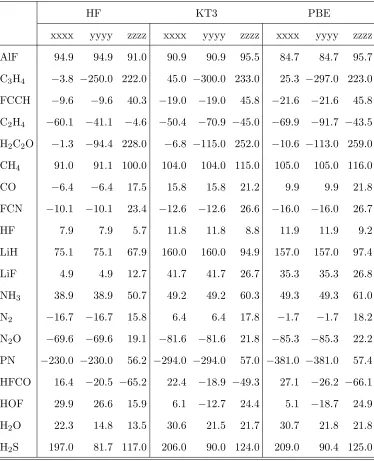
TABLE I. Hypermagnetizability tensor elements (SI a.u.) calculated using DFT functionals in the
aug-cc-pCVTZ basis set. The corresponding Hartree–Fock results are included for comparison.
Results are presented here for the subset of 19 molecules described in Section IV. Data for the full
set of 27 molecules may be found in the supplementary material48.
HF KT3 PBE
xxxx yyyy zzzz xxxx yyyy zzzz xxxx yyyy zzzz
AlF 94.9 94.9 91.0 90.9 90.9 95.5 84.7 84.7 95.7
C3H4 −3.8 −250.0 222.0 45.0 −300.0 233.0 25.3 −297.0 223.0
FCCH −9.6 −9.6 40.3 −19.0 −19.0 45.8 −21.6 −21.6 45.8
C2H4 −60.1 −41.1 −4.6 −50.4 −70.9 −45.0 −69.9 −91.7 −43.5
H2C2O −1.3 −94.4 228.0 −6.8 −115.0 252.0 −10.6 −113.0 259.0
CH4 91.0 91.1 100.0 104.0 104.0 115.0 105.0 105.0 116.0
CO −6.4 −6.4 17.5 15.8 15.8 21.2 9.9 9.9 21.8
FCN −10.1 −10.1 23.4 −12.6 −12.6 26.6 −16.0 −16.0 26.7
HF 7.9 7.9 5.7 11.8 11.8 8.8 11.9 11.9 9.2
LiH 75.1 75.1 67.9 160.0 160.0 94.9 157.0 157.0 97.4
LiF 4.9 4.9 12.7 41.7 41.7 26.7 35.3 35.3 26.8
NH3 38.9 38.9 50.7 49.2 49.2 60.3 49.3 49.3 61.0
N2 −16.7 −16.7 15.8 6.4 6.4 17.8 −1.7 −1.7 18.2
N2O −69.6 −69.6 19.1 −81.6 −81.6 21.8 −85.3 −85.3 22.2
PN −230.0 −230.0 56.2 −294.0 −294.0 57.0 −381.0 −381.0 57.4
HFCO 16.4 −20.5 −65.2 22.4 −18.9 −49.3 27.1 −26.2 −66.1
HOF 29.9 26.6 15.9 6.1 −12.7 24.4 5.1 −18.7 24.9
H2O 22.3 14.8 13.5 30.6 21.5 21.7 30.7 21.8 21.8
10
−1010
−510
0−4
−2
0
2
4
6
8
x 10
−4ρ
[au]
g(
ρ
) [au]
original
LHC
OMC
TP
TV
[image:26.612.91.498.82.421.2]HHx+HHc
10
−1010
−510
010
−1010
−810
−610
−4ρ
[au]
|g(
ρ
)| [au]
LHC
TV
HHmod
ρ
1/3
/100
[image:27.612.76.497.93.422.2]ρ
/1000
FIGURE CAPTIONS
Figure 1 : Different model functions g(ρ) used in the VRG functional.
Figure 2 : The low-density behaviour of three model functions g(ρ) used in the VRG
functional. The Higuchi–Higuchi exchange functional HHx has been reparametrized so that
the total exchange–correlation functional approaches zero for small densities; however, the
correlation functional HHc goes through a singularity and a sign shift atρ= 10−30 a.u.. The indicated asymptotic HHx+HHc behaviour therefore does not extend to this region.
Figure 3: Illustration of the errors in isotropic molecular magnetizabilities (10−30JT−2)
calculated using DFT functionals with and without the VRG(LHC) and VRG(TP)
correc-tions in the aug-cc-pCVTZ basis set. Results that failed to converge during SCF
optimiza-tion with the VRG(LHC) correcoptimiza-tions have been omitted. The grey boxes enclose one sample
standard deviation above and below the mean error. The mean error for each method is
indicated by a horizontal blue line. The plot markers show the individual errors for each of
the 19 molecules listed in Section IV.
Figure 4 : The VRG correction to the oxygen shielding constant in the water molecule
plotted against the integration regularization cut-off parameter ρcut-off for the LHC (left),
TP (middle), and HHmod (right) parameterizations of g(ρ) in Eq. (6). Both hard and soft
cut-offs are illustrated in the plots. The Huz-II basis, with London gauge factors, was used
in all cases.
Figure 5 : Illustration of the errors in isotropic shielding constants (ppm) calculated
using DFT functionals with and without the VRG(LHC) and VRG(TP) corrections in the
aug-cc-pCVTZ basis set. Results that failed to converge during the SCF optimization with
the VRG(LHC) correction have been omitted. The grey boxes enclose one sample standard
deviation above and below the mean error. The mean error for each method is indicated
by a horizontal blue line. The plot markers show the individual errors for each chemically
unique nuclei in the 19 molecules listed in Section IV (a total of 48 data points).
u-aug-cc-pVTZ basis set was used. Note that the curves have been aligned at R= 9 bohr.
Figure 7 : Dissociation curves for He2 subject to a perpendicular fieldB⊥= 1 au. The