Vol. 00, No. 00, Month 20XX, 1–21
Design of sliding mode observer for a class of uncertain neutral stochastic systems
Zhen Liua, b, Lin Zhaoc, Quanmin Zhud∗and Cunchen Gaoa
aSchool of Mathematical Sciences, Ocean University of China, Qingdao, China;bInstitute for Sustainable Manufacturing, College of Engineering, University of Kentucky, Lexington, USA;cCollege of Automation Engineering, Qingdao University, Qingdao, China;dDepartment of Engineering Design and Mathematics,
University of the West of England, Bristol, UK (Received 00 Month 20XX; final version received 00 Month 20XX)
The problem of robustH∞control for a class of uncertain neutral stochastic systems (NSS) is investigated by utilizing the sliding mode observer (SMO) technique. This paper presents a novel observer and integral-type sliding surface design, based on which a new sufficient condition guaranteeing the resultant sliding mode dynamics (SMDs) to be mean-square exponentially stable with a prescribed level ofH∞performance is derived. Then, an adaptive reaching motion controller is synthesized to lead the system to the predesigned sliding surface in finite-time almost surely. Finally, two illustrative examples are exhibited to verify the validity and superiority of the developed scheme.
Keywords:neutral stochastic systems; sliding mode control; non-fragile observer;H∞performance; stability
1. Introduction
Neutral systems, where the delays exist in both the system state and the state derivative, have been received great attention in the control community during the past decades, and arise in various applications (Hale, & Verduyn Lunel, 1993), e.g., the lossless transmission system, simultaneously. Thus, a great amount of studies have been devoted to the systems from a practical point of view, for instance, stability analysis (Karimi, 2011; Sakthivel, Mathiyalagan, & Anthoni, 2012) and control designs, which includeH∞filtering (Shen, Xu, Zhou, & Lu, 2011), guaranteed cost control (Parlakc, 2010), observer design (Elhsoumi, Ali, Bel, Harabi, & Abdelkrim, 2016), etc. In fact, for the more general case where the control matrix B is perturbed by some factors, i.e.,B(x, χ,t), whereχis an uncertain parameter vector (Hung, Gao, & Hung, 1993), the following uncertain neutral system is taken as example:
˙
x(t)−Dx˙(t−τ)= A(t)x(t)+Ad(t)x(t−d)+B(x, χ,t)u(t)+Gv(t), (1)
whereB(x, χ,t),B+ ∆B(χ,t)+g(x, χ,t) with the form of∆B(χ,t) andg(x, χ,t) as
∆B(χ,t)= B∆B˜(χ,t), g(x, χ,t)=B∆g˜(x, χ,t) (2)
for certain∆B˜(χ,t) and∆g˜(x, χ,t). Here, we recall the physical meaning of (2) is that all modeling uncer-tainties and disturbances enter the system through the control channel, i.e., the matched unceruncer-tainties in sliding mode control (SMC) theory (Hung et al., 1993). Thus, in the position, when subjected to some per-turbations or nonlinearities through the control channel of the system, the aforementioned control design methods may lose their reliable effects upon many occasions.
Emails: [email protected]; [email protected]; [email protected]
Conversely, SMC (Ahmad, & Zhu, 2015; Utikin, 1992), because of its various attractive features such as quick response, good transient performance, particularly, the valuable invariance against matched uncer-tainties, has been well known as an effective robust control strategy and also has found to be widely applied to various complex systems (Basin, Ferreira, & Fridman, 2007; Liu, & Gao, 2016; Wu, & Lam, 2008; Zhao, & Zhu, 2014) as well in many technical problems (Zhao, & Jia, 2015). As for the neutral systems, some excellent works have been reported. To name a few, SMC for uncertain neutral systems with structural un-certainties has been studied in Niu, Lam, & Wang (2004). In Gao, Liu, & Xu (2013), the problem of robust exponential stability for a class of uncertain neutral systems has been considered on the basis of an integral SMC approach. It is observed that, in spite of the availability of SMC, however, most of the reports are obtained upon the premise that all the system states are accessible. In many practical systems, it has been approved that the system states may not be totally acquired and even generally not easily to be evaluated through output measurement. In order to tackle these problems, by incorporating the superiority of the SMC with the observer effectively, the observer-based SMC technique, also called as the sliding mode observer (SMO) strategy (Rahme, & Meskin, 2015; Shi, Liu, & Zhang, 2015), has been developed to solve the state estimation issue for a variety of complex systems as well many realistic engineering plants successfully, see Kao, Li, & Wang (2014); Li, Shi, Yao, & Wu (2016); Liu, Gao, & Kao (2015); Wu, Wang, & Zeng (2008); Yan, Spurgeon, & Edwards (2010); Zhang, Shi, & Lin (2016) and the references therein. For instance, the SMO design for nonlinear uncertain neutral systems with unmeasured states has been perfectly investigated in Wu et al. (2008); afterwards, the observer-basedH∞ control scheme has been proposed for uncertain neutral systems via integral SMC in Liu et al. (2015).
On another research front, stochastic perturbations often exist in many real-world systems, and the ad-ditive stochastic effects result in a type of neutral stochastic systems (NSS) (Mao, 2007), see Eq. (3) in this paper, which play an important role in many industrial fields. In recent years, increasing efforts have been made to probe the NSS, the main research of which focuses on the stability analysis (e.g., stochastic stability and stability in the mean-square sense, etc) and control of the systems, e.g., Chen, Hu, & Wang (2014); Chen, & Shen (2009); Chen, Zheng, & Shen (2009); Chen, Zheng, & Xue (2010); Huang, & Mao (2009); Jankovic, Randjelovic, & Jovanovic (2009); Song, Xu, Xia, Zou, & Chen (2011); Song, Park, Wu, & Zhang (2013); Xu, Chu, Lu, & Zou (2006); Xu, Shi, Chu, & Zou (2006) and the references therein. It is noted that, SMC for uncertain NSS without matched uncertainties have been concerned by Chen, & Zhang (2008); Kao, Wang, Xie, Karimi, & Li (2015). Nevertheless, when uncertainties and/or perturbations ap-pear through the control channels, less research work has been involved on the NSS, which forms the first motivation of our concern.
In addition, consider that the system states may not be accessible on account of the factors (e.g., cost, technique, etc), so the SMO scheme shall be employed to deal with this case. More specifically, the observer-based SMC problem has been investigated for a class of NSS without the matched uncertain-ties, see Kao, Xie, Wang, & Karimi (2015); Li, & Li (2009), whereas the uncertainties are considered in the present work. Also, robust adaptive SMC for uncertain neutral Markovian jumped systems with un-measured states and unknown nonlinearity has been studied in Yao, Liu, Li, & Ma (2015), however, the state-dependent stochastic effect is not considered due to some difficulties therein. To the best of the authors knowledge, the issue remains open and challenging, and some problems may be still questions of common interest, then we hope to shorten such a gap, which is the second motivation of the paper. It should also be mentioned that, the matched ones has been done for deterministic neutral systems, where the general method is that: Both the controller itself and a discontinuous output error injection term (or called the con-troller compensator) are required to design for rejecting the uncertainties and guaranteeing robust stability of the closed-loop systems. In such case, the associated problems including the sliding surface design will be more complicated to configure. Moreover, because the techniques for deterministic neutral systems such as Liu et al. (2015); Wu et al. (2008) are not directly applicable to the NSS, another way should be adopted. To respond the above situations, the H∞ performance and mean-square exponential stability problem for a class of NSS with structural uncertainties, perturbation and external disturbance is investigated via a novel SMO scheme in this paper. The main contribution of the work is outlined below:
In detail, for most of the existing methods to handle the observer-based issues, main ideas are that: System stability is analyzed through the original system and its observer so as to ensure the error system to converge to the equilibrium state. Here, the new technical route is that: If the stability of the original system and its error system can be guaranteed, the observer states can tend to be stable as it is. Namely, the control problem will be achieved through the original system and its error system in the present scheme.
2). A particular nonfragile observer is established as the new SMO.
It is noted that, the SMO design, no matter for the deterministic neutral systems or the existing NSS, is generally developed with the so-called composite controller, i.e., the controller itself and its compensator (or the discontinuous output error injection term) are both required to satisfy the main goal. However, in this note, the composite controller will be no longer needed for SMO, and the resultant convenience is that: The controller is only performed in the original system part, and the actions of the error system and the observer will be responded automatically.
3). A novel single sliding surface is introduced for the scheme.
Compared with the previous designs, error terms are introduced in the present sliding surface design, which well performs to avoid difficulties caused by the perturbations through the control channel. This design may also benefit to highlight the attractive feature of SMC that the SMDs could be insensitive to all matched uncertainties. The design of the sliding surface for the NSS may be more interesting via the layout.
4). A novel adaptive sliding mode controller is presented.
Due to the state-dependent stochastic noises in the NSS, the techniques for deterministic neutral systems may not be directly applicable to the NSS. At this point, an adaptive controller is synthesized, where the outputs of the systems and its observer are involved, and the unknown bounds can be exactly tracked. Then, the expected performance of the closed-loop systems can be achieved.
The paper is organized as follows. Problem description and preliminaries are given in Section 2. Section 3 is arranged by the main results. Illustrative examples are provided to verify the theoretical result in Section 4. Conclusions are epitomized in Section 5.
Notation. Throughout the paper, the notationX > Y (respectively,X ≥ Y) means that the matrixX−Y is positive definite (respectively, positive semi-definite). (Ω,F,{Ft}t≥0,P) represents a completed probabil-ity space with a natural filtration{Ft}t≥0, whereΩis a sample space,F is theσ-algebra of subset of the
sample space, andPis the probability measure onF. Leth>0 andC([−h, 0];Rn) denote the family of all continuousRn-valued functions on [−h, 0]. LetCFb
0([−h, 0];R
n) be the family of all F
0-measurable
boundedC([−h, 0];Rn)-valued random variables. E{·} is the expectation operator with respect to some probability measureP. The superscript “T” denotes the transpose of a vector or matrix, and the symmetric elements of the matrix is denoted by “ * ”. sym{X}is denoted as sym{X} = X+ XT. If Mis a matrix, its operator norm is denoted by∥M∥=sup{∥M x∥:∥x∥=1},λmax(M) andλmin(M) represent its maximum and
minimum eigenvalues, respectively. Tr{·}denotes the trace of a matrix. diag{·}represents a block-diagonal matrix.L2[0,∞) stands for the space of square integral vector functions over [0,∞).
2. System description and preliminaries
Consider the followingn-dimensional neutral stochastic systems (NSS) described by
d[x(t)−Dx(t−τ)]={(A+ ∆A(t))x(t)+(Ad+ ∆Ad(t))x(t−d(t))
+B[u(t)+ f(t,x(t))]+Gv(t)}dt+g(t,x(t))dω(t),
y(t)=C x(t),
x(θ) =ϕ(θ), θ∈[−h, 0]
(3)
where x(t) ∈ Rn is the state vector,u(t) ∈ Rm is the control input, y(t) ∈ Rq is the system output.τ > 0 is a constant neutral-term time-delay,d(t) is the time-varying delay, which satisfies 0 < d(t) ≤ d and
˙
defined on a completed probability space (Ω,F,{Ft}t≥0,P) with a natural filtration{Ft}t≥0, and satisfies
E{dω(t)} = 0, E{dω2(t)} = dt. v(t) ∈ Rl represents a set of exogenous disturbance which belongs to
L2[0,∞).ϕ(t)∈CFb
0([−h, 0];R
n) is the initial condition.A,A
d,B,C,DandGare known real matrices,B is of full column rank, and the spectrum radius of the matrixD, i.e.,ρ(D), satisfiesρ(D) <1. To facilitate the result, the following preliminaries are introduced for the system (3).
Assumption 1. The structural uncertainties ∆A(t) and∆Ad(t) are norm bounded, i.e., [∆A(t) ∆Ad(t)] =
E J(t)[F Fd], where E, F and Fd are constant matrices, and J(t) is unknown matrix function satisfying
JT(t)J(t)≤ Ifor allt≥0.
Assumption 2. f(t,x) is unknown nonlinearity which represents the lumped perturbation of a physical plant through the control channel satisfying∥f(t,x)∥ ≤α∥y(t)∥, whereα >0 is an unknown constant (Li et al., 2016; Yao et al., 2015).
Assumption 3. The diffusion gain function g(t,x) may not be exactly known but there exist a matrix M
such that the inequality holds: Tr{gT(t,x)g(t,x)} ≤ ∥My(t)∥2.
Remark 1: The Assumption 3 is reasonable to a certain degree. Actually, the state-dependent stochastic noisesg(t,x) may not be accessible but could be evaluated by Tr{gT(t,x)g(t,x)} ≤ ∥N x(t)∥2, whereN is a constant matrix, see Huang, & Mao (2010); Kao et al. (2014, 2015). With the relevance thaty(t) =C x(t), i.e.,x(t)=C+y(t), the assumption is easily introduced herein, whereC+denotes the Moore-Penrose inverse ofC. Consider thatx(t) may be unmeasured, the output information is used to facilitate the control design. As toC, its selection may be flexible by the actual design, e.g., it can be of full column rank.
Based on above conditions, one can verify that the stochastic neutral system (3) with u(t) = 0 has a unique solution according to Huang et al. (2009); Mao (2007). In fact, denote the following terms:
m(t)=(A+ ∆A(t))x(t)+(Ad+ ∆Ad(t))x(t−d(t))+B f(t,x)+Gv(t), n(t)=g(t,x)
for allt ≥ 0. It is easy to observe that∥m(t)∥2 ≤ Km∥xt∥2,∥n(t)∥2 ≤ Kn∥xt∥2, where xt = {x(t+θ) : −h ≤
θ ≤ 0}, Km andKn are positive and can be found upon the premise of each component of m(t) andn(t), respectively. Thus, this implies m(t) and n(t) satisfy the local Lipschitz condition and the linear growth condition. At this point, there exists a unique continuous solution expressed byx(t;ϕ) to the NSS (3), and the details can refer to Theorem 3.1 of Mao (2007).
Definition 1: Chen et al. (2010): The system (3) is said to be mean-square exponentially stable if there exist scalarsη >0,β >0 such thatE{∥x(t)∥2} ≤ηe−βtsup−h≤θ≤0E{∥ϕ(θ)∥2}for all admissible uncertainties. Lemma 2.1: Huang et al. (2010): For a pair of constant matrices G∈Rp×pand M ∈Rp×q, if G≥0, then
Tr(MTGM)≤λmax(G)Tr(MTM).
3. Design of the sliding mode observer
3.1. Non-fragile state observer and novel sliding surface design
Firstly, the state observer technique is utilized to generate the accurate state estimation of the system (3). Here, the following non-fragile observer is employed for the design
d[ ˆx(t)−Dxˆ(t−τ)]={Axˆ(t)+Adxˆ(t−d(t))+(L+ ∆L(t))(y(t)−Cxˆ(t))}dt, ˆ
y(t)=Cxˆ(t), ˆ
x(θ)=ϕˆ(θ), θ∈[−h, 0]
(4)
where ˆx(t) ∈ Rnrepresents the estimation of x(t), ˆy(t) denote the output of the observer.L ∈ Rn×p is the observer gain to be designed later, and∆L(t) is an additive gain variation satisfying∥∆L(t)∥ ≤ δ, where
δ >0 is a constant, namely, the observer may be affected by some perturbations (Kao et al., 2014, 2015).
Let the estimation error bee(t)= x(t)−xˆ(t). Thus, by subtracting (4) from (3), one can get the following estimation error system
d[e(t)−De(t−τ)]={[A−LC−∆L(t)C]e(t)+Ade(t−d(t))+ ∆A(t)x(t)
+∆Ad(t)x(t−d(t))+B[u(t)+ f(t,x(t))]+Gv(t)}dt+g(t,x(t))dω(t),
ye(t)=Ce(t)
(5)
whereye(t) denotes the output of the error system.
Remark 2: In this work, a particular non-fragile observer is proposed for the system. Different from previ-ous designs of the observer, see Elhsoumi et al. (2016); Kao et al. (2014, 2015); Li et al. (2016, 2009); Lin, Wang, Lee, He, & Chen (2008); Liu et al. (2015); Qiao, Zhang, Zhu, & Zhang (2009); Rahme et al. (2015); Shi et al. (2015); Wu et al. (2008); Yan et al. (2010); Yao et al. (2015); Zhang et al. (2016) for details, it is worth noting that the control input and/or its compensator are both required to involve into their observer design, however, only an observer gainLis to be determined here. Thus, this simplified the procedure of the state observer design, which is thefirstadvantage of this paper.
Now, a novel integral-type sliding surface function is defined as follows:
s(t)= H[e(t)−De(t−τ)]+H[ ˆx(t)−Dxˆ(t−τ)]− ∫ t
0
H(A+BK) ˆx(θ)dθ, (6)
where the gain matrixKis to be determined.H ∈Rm×nis a known matrix satisfyingHBis non-singular. And it is assumed that the matrixHmatches the following requirement:
H=N1C, HD= N2C (7)
whereN1andN2are matrices to be determined. In order to enhance the freedom of the control scheme, we introduceH= BTZwith anyZ>0 to benefit the entire goal.
Remark 3: From the above discussion, the problem of unknown matricesN1andN2should be solved so that the sliding surface function (6) can be expressed by
s(t)=N1[y(t)−yˆ(t)]−N2[y(t−τ)−yˆ(t−τ)]+H[ ˆx(t)−Dxˆ(t−τ)]− ∫ t
0
H(A+BK) ˆx(θ)dθ,
if the condition (7) is exploited. In detail, it is seen that the solution ofN1andN2depends onC,DandH
3.2. Exponential stability analysis of the SMDs withH∞performance
In light of the trivial solution of the original system (3) and the error system (5), it could definitely be seen thats(t) is an It ˆostochastic process satisfying
ds(t)=Hd[e(t)−De(t−τ)]+Hd[ ˆx(t)−Dxˆ(t−τ)]−H(A+BK) ˆx(t)dt
=Ls(t)dt+Hg(t,x(t))dω(t) (8)
where
Ls(t)=HAe(t)+HAdx(t−d(t))+H∆A(t)x(t)+H∆Ad(t)x(t−d(t))+HB[u(t)+ f(t,x)]
+HGv(t)−HBKxˆ(t).
To achieve the sliding motion, an equivalent controller will be derived via the SMC theory (Huang et al., 2010; Utikin, 1992), i.e.,Es(t) = 0 and d(Edst(t)) = 0, that is to say,Ls(t) = 0 should be ensured from the conditionE{dω(t)}=0. Therefore, the so-called equivalent controller can be obtained by
ueq(t)=Kxˆ(t)− f(t,x)−(HB)−1[HAe(t)+HAdx(t−d(t))+H∆A(t)x(t)
+H∆Ad(t)x(t−d(t))+HGv(t)]. (9)
Substituting (9) into the system (3), one gets the dynamic equation of the original system (3) in the sliding mode as follows
d[x(t)−Dx(t−τ)]={[A+BK+BH∆A(t)]x(t)+BH[Ad+ ∆Ad(t)]x(t−d(t))
−(BK+BA)e(t)+GBv(t)}dt+g(t,x)dω(t) (10)
whereBH =I−B(HB)−1H,BA=B(HB)−1HA,GB =BHG. Similarly, together with (9) and (5), the related dynamic equation of the error system (5) in the sliding mode can be described by
d[e(t)−De(t−τ)]={[AB−LC−BK−∆L(t)C]e(t)+Ade(t−d(t))+[BK+BH∆A(t)]x(t)
+[BH∆Ad(t)−Bd]x(t−d(t))+GBv(t)}dt+g(t,x)dω(t) (11)
whereAB=A−BA,Bd =B(HB)−1HAd.
Based on the above statement, it follows that (10) and (11) can be acknowledged as the sliding mode dynamics (SMDs) of the closed-loop systems. Then, the stability of the system (3) will be investigated through the SMDs (10)-(11) by resorting to adaptive SMC.
Remark 4: In this part, a novel integral-type sliding surface function in (6) is constructed. What really makes the design special can be listed in the following two aspects:
(i) Different from the forms proposed in Chen et al. (2008); Gao et al. (2013); Kao et al. (2015); Li et al. (2009); Liu et al. (2015); Niu (2004); Yao et al. (2015), the error termse(t) and De(t−τ) are introduced in the sliding surface design, which thoroughly performs to avoid difficulties caused by the perturbations through the control channel (i.e., f(t,x)), as can be seen from the derivative of the SMDs (10)-(11). This design may also benefit to highlight the attractive feature of SMC that SMDs can be insensitive to all matched uncertainties;
In conclusion, the design of the sliding surface for NSS is simplified via the present layout, which is seen as thesecondadvantage of the paper.
Remark 5: It should be mentioned that, as the observer (4) is applied, the control inputu(t) is embedded into the error system (5) as virtual controller. By utilizing the SMC method, stability analysis of the original system (3) is transformed into that of the overall closed-loop systems composed of the system (3) and its error system (5) in the sliding mode at the same time, so as to achieve the aim of the entire system control. This technical route is different from that of the existing SMO scheme, please refer to Kao et al. (2014, 2015); Li et al. (2016, 2009); Liu et al. (2015); Qiao et al. (2009); Rahme et al. (2015); Shi et al. (2015); Wu et al. (2008); Yan et al. (2010); Yao et al. (2015); Zhang et al. (2016) for more details, which may be thethirdmerit in the paper.
Specifically, the objective of robustH∞performance analysis studied in this note can be summarized as two purposes: on the basis of adaptive SMO method such that:
(P1) Given a positive scalarγ >0, the followingH∞performance index is satisfied
E sup
0,v(t)∈L2[0,∞)
∥ye(t)∥2/∥v(t)∥2< γ (12)
under zero initial conditions;
(P2) The SMDs (10)-(11) is mean-square exponentially stable withv(t)=0.
In this work, we call the SMDs in (10)-(11) satisfying (P1) and (P2) is mean-square exponentially stable withH∞disturbance attenuation levelγ. In terms of LMIs, the following sufficient criteria which guaran-tees the desirable performance can be derived.
Theorem 3.1: Consider the sliding surface function defined in (6) and the SMDs in (10)-(11). Given a scalarγ > 0, the SMDs is mean-square exponentially stable withH∞ disturbance attenuation levelγ, if there exist symmetric definite matrices P, Q1, Q2, R1, and R2, matrices X and Y, positive scalarsϱandεi
(i=1, . . . ,6) satisfying the following LMIs:
P< ϱI, (13)
Π11 Π12 Π13 Π14 −XTD 0 PGB Υ1
∗ −τQ1 Π23 Π24 0 0 −DTPGB Υ2
∗ ∗ Π33 −(PBd)T (PBd)TD 0 0 0
∗ ∗ ∗ Π44 Π45 PAd PGB Υ3
∗ ∗ ∗ ∗ −τR1 −DTPAd −DTPGB Υ4
∗ ∗ ∗ ∗ ∗ Π66 0 0
∗ ∗ ∗ ∗ ∗ ∗ −γ2I 0
∗ ∗ ∗ ∗ ∗ ∗ ∗ Υ5
<0, (14)
whereΠ11 = sys{PA+X} +τQ1 +dQ2+2ϱCTMTMC+(ε1+ ε2 +ε3+ε4)FTF, Π12 = −(PA+X)TD,
Π13=PBHAd+(ε1+ε2+ε3+ε4)FTFd,Π14= −X−PBA+XT,Π23= −DTPBHAd,Π24= DT(X+PBA),
Π33=−d(1−µ)Q2+(ε1+ε2+ε3+ε4)FTdFd,Π44=sys{PAB−YC−X}+τR1+dR2+CTC+(ε5+ε6)δ2CTC,
Π45=(−PAB+YC+X)TD,Π66= −d(1−µ)R2,Υ1=[PBHE 0 0 0 0 0],Υ2=[0 DTPBHE 0 0 0 0],
Υ3=[0 0 PBHE 0 P 0],Υ4 =[0 0 0 DTPBHE 0 DTP],Υ5 =diag{−ε1I,−ε2I,−ε3I,−ε4I,−ε5I,−ε6I}.
Proof. To begin with, choose the following Lyapunov function candidate
V(t) = [x(t)−Dx(t−τ)]TP[x(t)−Dx(t−τ)]+τ ∫ t
t−τ
xT(θ)Q1x(θ)dθ+d
∫ t
t−d(t)
xT(θ)Q2x(θ)dθ
+[e(t)−De(t−τ)]TP[e(t)−De(t−τ)]+τ ∫ t
t−τ
eT(θ)R1e(θ)dθ+d
∫ t
t−d(t)
eT(θ)R2e(θ)dθ.
In the light of It ˆodifferential formula (Mao, 2007), the stochastic differential ofV(t) is obtained as
dV(t)=LV(t)dt+2[x(t)−Dx(t−τ)+e(t)−De(t−τ)]TPg(t,x(t))dω(t) (15) with the infinitesimal operator
LV(t) = 2[x(t)−Dx(t−τ)]TP(A+BK)x(t)+BHAdx(t−d(t))−(BK+BA)e(t)
+GBv(t)]+2[x(t)−Dx(t−τ)]TPBH[∆A(t)x(t)+ ∆Ad(t)x(t−d(t))]
+τxT(t)Q1x(t)−τxT(t−τ)Q1x(t−τ)+dxT(t)Q2x(t)−d(1−d˙(t))
·xT(t−d(t))Q2x(t−d(t))+2[e(t)−De(t−τ)]TP[(AB−LC−BK)e(t)
+Ade(t−d(t))+BK x(t)−Bdx(t−d(t))+GBv(t)]+τeT(t)R1e(t)
−τeT(t−τ)R1e(t−τ)+deT(t)R2e(t)−d(1−d˙(t))eT(t−d(t))R2e(t−d(t))
+Tr{2gT(t,x)Pg(t,x)} −2[e(t)−De(t−τ)]TP∆L(t)Ce(t)+2[e(t)−De(t−τ)]T
·PBH[∆A(t)x(t)+ ∆Ad(t)x(t−d(t))]. (16)
Then, the following will be obtained by utilizing some inequality techniques
2xT(t)P BH[∆A(t)x(t)+ ∆Ad(t)x(t−d(t))]=2xT(t)PBHE J(t)[F x(t)+Fdx(t−d(t))]
≤ε−1
1 x T
(t)PBHEETBTHPx(t)+ε1[F x(t)+Fdx(t−d(t))]T[F x(t)+Fdx(t−d(t))], (17)
−2xT(t−τ)DTP BH[∆A(t)x(t)+ ∆Ad(t)x(t−d(t))]≤ε−21x T
(t−τ)DTPBHEETBTHPDx(t−τ)
+ε2[F x(t)+Fdx(t−d(t))]T[F x(t)+Fdx(t−d(t))], (18)
2eT(t)P BH[∆A(t)x(t)+ ∆Ad(t)x(t−d(t))]=eT(t)PBHE J(t)[F x(t)+Fdx(t−d(t))]
≤ε−1
3 e T
(t)PBHEETBTHPe(t)+ε3[F x(t)+Fdx(t−d(t))]T[F x(t)+Fdx(t−d(t))], (19) and
−2eT(t−τ)DTP BH[∆A(t)x(t)+ ∆Ad(t)x(t−d(t))]≤ε−41e
T(t−τ)DTPB
HEETBTHPDe(t−τ)
+ε4[F x(t)+Fdx(t−d(t))]T[F x(t)+Fdx(t−d(t))], (20)
In addition, it follows that
−2[e(t)−De(t−τ)]TP∆L(t)Ce(t)≤ε−51eT(t)PPe(t)+ε−61eT(t−τ)DTPPDe(t−τ)
+(ε5+ε6)δ2eT(t)CTCe(t). (21)
With the condition (13), Assumption 3 and Lemma 2.1, one can get
By incorporating (17)-(22) into (16), it results in
yTe(t)ye(t)−γ2vT(t)v(t)+LV(t)≤ζT(t)Ξζ(t) (23) where ζT(t)=[xT(t) xT(t−τ) xT(t−d(t)) eT(t) eT(t−τ) eT(t−d(t)) vT(t)],
Ξ=
Ξ11 Ξ12 Ξ13 Ξ14 −(PBK)TD 0 PGB
∗ Ξ22 −DTPBHAd Ξ24 0 0 −DTPGB
∗ ∗ Ξ33 −(PBd)T (PBd)TD 0 0
∗ ∗ ∗ Ξ44 Ξ45 PAd PGB
∗ ∗ ∗ ∗ Ξ55 −DTPAd −DTPGB
∗ ∗ ∗ ∗ ∗ Ξ66 0
∗ ∗ ∗ ∗ ∗ ∗ −γ2I
with
Ξ11 = sys{PA+PBK}+τQ1+dQ2+ 2ϱCTMTMC+ε−11PBHEETBTHP+(ε1 +ε2+ε3+ε4)FTF, Ξ12 =
−[P(A+BK)]TD,Ξ13= PBHAd+(ε1+ε2+ε3+ε4)FTFd,Ξ14 =−P(BK+BA)+(PBK)T,Ξ22 =−τQ1+
ε−1 2 D
TPB
HEETBTHPD,Ξ24=DTP(BK+BA),Ξ33=−d(1−µ)Q2+(ε1+ε2+ε3+ε4)FdTFd,Ξ44=sys{P(AB−
LC−BK)}+τR1+dR2+CTC+ε−31PBHEETBTHP+ε5−1PP+(ε5+ε6)δ2CTC,Ξ45=−[P(AB−LC−BK)]TD,
Ξ55=−τR1+ε−41DTPBHEETBTHPD+ε− 1 6 D
TPPD,Ξ
66=−d(1−µ)R2.
Then, denoteX = PBK,Y = PL. By applying the Schur complement, it is shown thatΞ <0is equivalent to the condition (14). In other word, if the LMIs (13) and (14) are established, one can get
LV(t)≤ −yTe(t)ye(t)+γ2vT(t)v(t). (24)
Therefore, by taking the zero initial conditions into account, it followsV(0)= 0. The following inequality can be obtained by integrating (24) with respect to timetfrom 0 to∞and taking mathematical expectation of both sides of it, simultaneously, which turns out
0≤E{V(∞)}=E{ ∫ ∞
0
LV(t)dt} ≤ −E{
∫ ∞
0
yTe(t)ye(t)dt}+γ2 ∫ ∞
0
vT(t)v(t)dt. (25)
The inequality indicatesE {sup0,v(t)∈L2[0,∞)∥ye(t)∥2/∥v(t)∥2
}
< γ, i.e.,P1can be guaranteed.
Next, the stability of the SMDs will be considered withv(t)=0. In the position, the following inequality can be easily obtained:eT(t)CTCe(t)+LV(t)=ξT(t)Θξ(t),
whereξT(t)=[xT(t) xT(t−τ) xT(t−d(t)) eT(t) eT(t−τ) eT(t−d(t))],Θis the first-six block of the matrix
Ξ, i.e., it is constituted by the first six lines and six columns ofΞ. Obviously, the condition (14) implies thatΘ<0, which shows thatLV(t)≤ξT(t)Θξ(t)<0, ifξ(t),0. Letκ=λmin{−Θ}>0, it is followed that
E{dV(t)
dt }=E{LV(t)} ≤ −κE{∥x(t)∥
2}.
(26)
Moreover, by virtue ofV(t), there surely exist finite positive scalarsα1,α2such that
α1∥x(t)∥2≤V(t) ≤α2∥x(t)∥2
which impliesE{∥x(t)∥2} ≥α−1
2 E{V(t)}. Thus, it follows that
E{dV(t)
dt } ≤ −κE{∥x(t)∥
2} ≤ −κα−1
2 E{V(t)}. (27)
Further, it is also held that a scalarα >0 can be found such that the following can be satisfied:
E{V(0)} ≤αsup−h≤θ≤0E{∥ϕ(θ)∥ 2}.
By integrating both sides of (27) over the interval [0, t] and invoking (28) as well, it follows that
E{∥x(t)∥2} ≤α1−1E{V(t)} ≤α−11E{V(0)}e−κα−21t ≤αα−1
1 e−κα
−1 2 tsup
−h≤θ≤0E{∥ϕ(θ)∥ 2}.
(29)
Denoteη = αα−1
1 andβ = κα− 1
2 . The system (10) is exponentially mean-square stable by Definition 1. In
like manner, one can prove the mean-square exponential stability of the system (11), thereby completing
the proof.
Remark 6: Theorem 3.1 gives a new criteria for the mean-square exponential stability of the closed-loop systems by employing the SMO approach, which can be regarded as an alternative to the gain matrices
K andL. It is worth noting that the LMIs (13)-(14) are linear in the set of matrices ofP,Q1,Q2,R1,R2,
X andY, positive scalarsϱ,εi (i=1, , 6) andγ2, which implies that the scalarλ = γ2 can be included as one of the optimization variables in LMIs (13)-(14) so as to minimize the parameter to reduce the effects of disturbances (i.e., to get the minimum disturbance attenuation level). Then, the optimal solution to the SMO scheme can be obtained by solving the following convex optimization problem:
min λ, subject to (13)−(14).
Remark 7: It should be mentioned that, SMO design for a class of NSS with Markovion jumping parame-ters has been developed in Kao et al. (2015); andH∞integral SMC problem for uncertain neutral systems has been studied based on the state observer in Liu et al. (2015). Yet, the reports did not involve the case that the nonlinearity and/or perturbation appear through the control channel. In this study, the uncertainties or unknown perturbations (i.e., f(t,x) through the control channel of the systems are concerned, and the complicated case can still be handled, whereas Kao et al. (2015); Liu et al. (2015) may not act, which implies the superiority and practicability of the proposed approach.
Remark 8: Now, the general algorithm to solve the LMIs in (13)-(14) which is subjected to the equality constraint (7) will be proposed. Similar to that of Li et al. (2016); Wu et al. (2008), the following optimal minimum problem is summarized to solve the undetermined parameters in Theorem 3.1 as well as the matricesN1andN2in (7):
min ηi(i[=1,2), subject to,(13)−(14),
−η1I (BTZ−N1C)T
∗ −I
]
<0, [
−η2I (BTZD−N2C)T
∗ −I
]
<0.
It is seen that the design is now changed to a minimization problem involving LMIs constraints and linear objective which can be achieved by using the Matlab software. Ifηiequals or tends to zero, the condition (7) can be guaranteed. The verbatim argument is omitted here for brevity.
3.3. Reachability analysis of sliding mode
In the following, the attention is focused on an adaptive controller synthesis, by which the sliding mode reachability of the systems trajectories can be ensured so that the system can start its sliding motion to be mean-square exponentially stable with a specificH∞disturbance attenuation level. To facilitate the result, the following assumptions are given.
Assumption 4. (Wu et al., 2008) Unknown positive scalarqcan be found to satisfy the following inequality:
Since the system statesx(t) are not completely available, the errore(t) may not be computable based on the fact, which is often the case in practical systems. Then, with the relationships among the system states
x(t), the errore(t), the outputsy(t) and ˆy(t), the following can be valid to a certain degree:
x(t)=C+y(t),ande(t)=C+(y(t)−yˆ(t)). (31)
Then, the assumption as follows will be reasonably given by togethering with the Assumption 2, 4 and (31).
Assumption 5. Unknown scalarsci>0 (i=1,2) can be found to satisfy the following estimation:
Z = ∥HA∥∥e(t)∥+∥HAd∥∥x(t−d(t))∥+∥H∆A(t)∥∥x(t)∥
+∥H∆Ad(t)∥∥x(t−d(t))∥+∥HB∥∥f(t,x)∥
≤ c1∥y(t)∥+c2∥yˆ(t)∥, t≥0. (32)
Notice that the estimation boundsc1andc2are not accessible in design process. Let ˆci(t) (i= 1,2) be the associated estimations of them with error parameters being ˜ci(t)=cˆi(t)−ci, respectively.
Theorem 3.2: Suppose that the integral sliding surface function is designed by (6), the gain matrix K is obtained by Theorem 3.1. The finite-time reachability of the desirable sliding mode can be guaranteed, if the adaptive SMC law in (33) is synthesized
u(t) = Kxˆ(t)−(HB)−1[ˆc1(t)∥y(t)∥+c2ˆ (t)∥yˆ(t)∥+∥HG∥∥v(t)∥+ρ
+λmax(HTH)∥My(t)∥2/∥s(t)∥]sgn(s(t)), (33)
where the updating laws are designed by c1˙ˆ (t) = λ1∥y(t)∥, c2˙ˆ (t) = λ2∥yˆ(t)∥, and λi > 0 (i = 1,2) are
constants as the adaptive gains chosen by the designer, andρ is a small positive constant. Moreover, the adaptive parameters can be denoted by the integral forms as:
ˆ
c1(t)=c1ˆ (0)+λ1
∫ t
0
∥y(τ)∥dτ, c2ˆ (t) =c2ˆ (0)+λ2
∫ t
0
∥yˆ(τ)∥dτ
wherecˆi(0)(i=1,2) are the initial values of the adaptive estimates, without loss of generality,cˆi(0)can be
zero for simplicity.
Proof. Choose a Lyapunov function candidate
˜
V(t,s(t))=(sT(t)s(t))12 +0.5[λ−1
1 c˜ 2 1(t)+λ−
1 2 c˜
2
2(t)]=∥s(t)∥+0.5[λ− 1 1 c˜
2 1(t)+λ−
1 2 c˜
2 2(t)].
By the It ˆoformula, one has
d ˜V(t,s(t))=LV˜(t,s(t))dt+ s T(t)
∥s(t)∥Hg(t,x(t))dω(t)
where
LV˜(t,s(t)) = sT(t)
∥s(t)∥{HAe(t)+HAdx(t−d(t))+H∆Ax(t)+H∆Ad(t)
·x(t−d(t))+HB[u(t)+ f(t,x)]+HGv(t)−HBKxˆ(t)}
+1
2g
T(t,x(t))HT
{
Im
∥s(t)∥−
s(t)sT(t)
∥s(t)∥3
}
Hg(t,x(t)))
+λ−1
1 c1˜ (t)˙˜c1(t)+λ− 1
Substituting (33) into (34) and employing some inequality technique yields
LV˜(t,s(t)) = 1
∥s(t)∥s
T
(t){HAe(t)+HAdx(t−d(t))+H∆Ax(t)+H∆Ad(t)x(t−d(t))
+HB f(t,x)+HGv(t)−[ˆc1(t)∥y(t)∥+c2ˆ (t)∥yˆ(t)∥+∥HG∥∥v(t)∥+ρ
+λmax(HTH)∥My(t)∥2/∥s(t)∥]sgn(s(t))}+
1 2g
T(t,x(t))HT
·
{
Im
∥s(t)∥−
s(t)sT(t)
∥s(t)∥3
}
Hg(t,x(t))+λ1−1c1˜ (t)˙˜c1(t)+λ− 1
2 c2˜ (t)˙˜c2(t)
≤ ∥ 1
s(t)∥∥s(t)∥{∥HA∥∥e(t)∥+∥HAd∥∥x(t−d(t))∥+∥H∆A(t)∥∥x(t)∥+∥H∆Ad(t)∥
·∥x(t−d(t))∥+∥HB∥∥f(t,x)∥+∥HGv(t)∥} − 1
∥s(t)∥[ˆc1(t)∥y(t)∥+c2ˆ (t)∥yˆ(t)∥
+∥HG∥∥v(t)∥+ρ+λmax(HTH)∥My(t)∥2/∥s(t)∥]sT(t)sgn(s(t))+
1
∥s(t)∥
·∥gT(t,x(t))HTHg(t,x(t))∥+λ1−1c1˜ (t)˙˜c1(t)+λ2−1c2˜ (t)˙˜c2(t)
≤ c1∥y(t)∥+c2∥yˆ(t)∥+∥HGv(t)∥ − {c1ˆ (t)∥y(t)∥+c2ˆ (t)∥yˆ(t)∥+∥HG∥∥v(t)∥
+ρ+λmax(HTH)∥My(t)∥2/∥s(t)∥}+
1
∥s(t)∥∥g
T(t,x(t))HTHg(t,x(t))∥
+λ−1
1 c1˜ (t)˙˜c1(t)+λ− 1
2 c2˜ (t)˙˜c2(t).
Notice that the following terms keep valid
˙ˆ
c1(t)=c1˙˜ (t), c2˙ˆ (t)=c2˙˜ (t). (35)
Then, in view of Lemma 2.1, and taking (35) into consideration, it follows
LV˜(t,s(t)) ≤ c1∥y(t)∥+c2∥yˆ(t)∥ −c1ˆ ∥y(t)∥ −c2ˆ ∥yˆ(t)∥ −ρ−λmax(HT
H)∥My(t)∥2/∥s(t)∥
+∥ 1
s(t)∥∥g
T(t,x(t))HTHg(t,x(t))∥+λ−1
1 c1˜ (t)˙˜c1(t)+λ− 1
2 c2˜ (t)˙˜c2(t)
≤ −c1˜ (t)∥y(t)∥ −c2˜ (t)∥yˆ(t)∥ −ρ+λ−11c1˜ (t)˙˜c1(t)+λ−21c2˜ (t)˙˜c2(t)
= −ρ. (36)
Thus, by integrating (36) from 0 totand taking expectation for both sides, one can testify that
E∥s(t)∥ ≤EV˜(t,s(t))≤EV˜(0,s(0))−ρt,
which implies E∥s(t)∥ = 0 for all t ≥ tf = E
˜
V(0,s(0))
ρ . Furthermore, it follows that ∥s(t)∥ = 0 can be
established in finite-time almost surely. The proof is completed.
Remark 9: A novel adaptive sliding mode controller is presented for the NSS, which does not rely on the information of the delayed state, while the design in Kao et al. (2015); Li et al. (2009); Yao et al. (2015) is absolutely a memory controller. Besides, because of the state-dependent stochastic noise in the NSS, the techniques for deterministic neutral systems such as Liu et al. (2015); Wu et al. (2008); Yao et al. (2015) will not be directly applicable to the NSS. Thus, the adaptive controller is synthesized in (33), where the outputs of the systems and its observer are involved based on the information among x(t),e(t), y(t) and ˆ
the control input is regarded as virtual controller in the error system. This is thefourth highlight of the scheme.
Remark 10: As is seen, a particular state observer has been introduced to estimate the system states, where the observer is designed without any switching terms, and the control input and discontinuous output error injection term (or called the controller compensator) are no longer needed. Based on the observer, the SMC approach is utilized to force the trajectories of the original system and the error system to stay on the predesigned sliding surface almost surely despite the existence of perturbations, thus enabling the closed-loop systems to reject the uncertainties and disturbances when specified conditions are satisfied.
In conclusion, the developed observer-based SMC design for the NSS can be seen as a supplement of the SMO strategy.
4. Illustrative examples
As is mentioned in the introduction, many physical systems in industrial fields such as lossless transmis-sion lines, collitransmis-sion problem in electrodynamics can be modeled by neutral stochastic differential functional equations when stochastic perturbations are taken into account, which is often inevitable in practical engi-neering. Thus, the stability analysis and numerical treatment of such systems may be of great importance (Mao, 2007), particularly when there is a need for their control. As a practical application, a general de-scription of the shunted transmission line (see the pages 5 and 6 in Hale.et al. (1993)) was presented, which could be modeled by a type of NSS with the following form:
d[x(t)−Dx(t−τ)]=m(t,x(t),x(t−τ))dt+n(t)dω(t)
whereτ=2/√UV,UandV are the mutual capacity and inductance of the line, respectively. In particular, it will be the form of (3) by the selection of
m(t,x(t),x(t−τ))=(A+ ∆A(t))x(t)+(Ad+ ∆Ad(t))x(t−τ)+B[u(t)+ f(t,x(t))]+Gv(t),
n(t)=g(t,x(t)).
Thus, the following Example 1 is firstly introduced with the above discussion.
Example 1. (MIMO system) Let us consider the NSS with the parameters given by Example 4 of Chen et al. (2009) as follows:
D=
[
0.1 0 0 0.1
]
,A=
[
−0.7 0.2
0.3 0.1 ]
,Ad =
[
0.2 0 0.1 −0.1
]
,B=
[
−0.2 1
0 0.7 ]
,
E= F= Fd =0,C = [
−0.1 0
0.2 0.1 ]
,G=
[ 1 1
]
.
The time-delays are chosen byτ=d=1 withµ=0. The additive gain variation of the observer is assumed as∆L(t) = diag{0.15sint,−0.2sint}, and δ can be set as 0.2. With the above parameters, the following solutions are obtained by solving the minimization problem in Remark 8 forγ = 0.0517, M = 1.25, and
Z=
[
2.5 1 1 5
]
as follows:
η1=η2=8.0167·10−16(So, the condition (7) can be ensured), andN1=
[
1.0 −2.0 58 45
] ,N1 =
[
0.1 −0.2 5.8 4.5
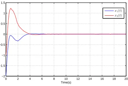
0 2 4 6 8 10 12 14 16 18 20 −2
−1.5 −1 −0.5 0 0.5 1 1.5
Time(s)
[image:14.595.196.404.66.206.2]x1(t) x2(t)
Figure 1. Evolution of the system state
Then, the associated gain matrices can be computed by
L=
[
−10.6029 14.6571
30.6019 34.8072 ]
, K=
[
−6.8782 −8.4728
−3.0624 −2.6059
]
.
At this point, we set the adaptive gainsλ1 = 2.0,λ2 = 2.5, andρ = 2.5. Thus, the integral sliding surface
and adaptive sliding mode controller are designed as
s(t) = N1[(y(t)−yˆ(t)]−N2[y(t−1)−yˆ(t−1)]+ [
−0.5 −0.2
3.2 4.5 ]
[ ˆx(t)− [
0.1 0 0 0.1
] ˆ
x(t−1)]
−
∫ t
0
[
1.5621 0.7005
−15.9343 −10.0349
] ˆ
x(θ)dθ
and
u(t) = [
−6.8782 −8.4728
−3.0624 −2.6059
] ˆ
x(t)+[ˆc1(t)∥y(t)∥+c2ˆ (t)∥yˆ(t)∥+7.7318∥v(t)∥+2.5
+47.9619∥y(t)∥2/∥s(t)∥]sgn(s(t)) with the updating laws given by
˙ˆ
c1(t)=2.0∥y(t)∥, c2˙ˆ (t)=2.5∥yˆ(t)∥.
Moreover, the system is assumed to subject to the nonlinear perturbation, the external disturbance given by
f(t,x) = [
0 −√3cos2t+1 sint−1 0
]
x(t), v(t)=−0.15sint·e−0.5t, and
the state-dependent stochastic effect gain function g(t,x) is also the same one in Chen et al. (2009). Simulation results are provided in Figs. 1-5 under the initial conditions x(θ) = [ −2.0 −1 ]T, and
ˆ
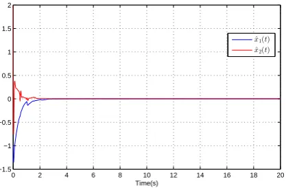
[image:14.595.64.513.359.499.2]0 2 4 6 8 10 12 14 16 18 20 −3
−2.5 −2 −1.5 −1 −0.5 0 0.5 1 1.5
Time(s)
ˆ
x1(t) ˆ
[image:15.595.196.405.66.204.2]x2(t)
Figure 2. Evolution of the state observer
0 2 4 6 8 10 12 14 16 18 20
−12 −10 −8 −6 −4 −2 0 2
Time(s)
s1(t)
[image:15.595.198.404.255.391.2]s2(t)
Figure 3. The sliding surface function
0 2 4 6 8 10 12 14 16 18 20
−10 −5 0 5 10 15 20 25
Time(s)
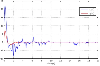
u1(t)
u2(t)
Figure 4. The control inputs
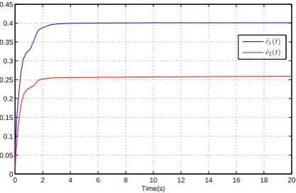
[image:15.595.197.405.443.580.2]0 2 4 6 8 10 12 14 16 18 20 0 0.1 0.2 0.3 0.4 0.5 0.6 0.7 Time(s) ˆ
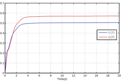
c1(t) ˆ
[image:16.595.197.404.65.207.2]c2(t)
Figure 5. The estimated values
Example 2. (SISO system) The considered uncertain NSS (3) are given with the following data:
D=
[
0.1 0 0 0.1
]
,A=
[
−2.0 2.5
0 1.5 ]
,Ad=
[
1.0 1.5 2.0 −2.0
]
,B=
[ 0 1
]
,G=
[
−0.2 0.1
]
,
E =
[
−0.2 0
0 0
]
,F=
[
0.1 0 0 −0.2
]
,Fd =
[
0.2 0 0 0.1
]
,C=[ 0 1 ].
The time-delays are chosen byτ = 0.5,d = 1 withµ = 0. The additive gain variation of the observer is
assumed as∆L(t)=[ 0.12sint 0 ]T, andδcan be set as 0.12. For brevity, we select the matrixZto be the identity matrix, soN1andN2are easily obtained asN1= 1 andN2=0.1. Givenγ=0.5212,M =1.5, the corresponding gain matrices are computed by Theorem 1 as follows
L= [ 10.1660 62.9185 ]T,K =[ −7.9271 −39.9163 ].
Letλ1 = 2.0, λ2 = 1.5, and ρ = 1.75. Hence, the designed sliding surface and adaptive controller are
presented by
s(t) = [y(t)−yˆ(t)]−0.1[y(t−0.5)−yˆ(t−0.5)]+[0 1.0][ ˆx(t)− [
0.1 0 0 0.1
] ˆ
x(t−0.5)]
+
∫ t
0
[
7.9271 38.4163 ]xˆ(θ)dθ.
and
u(t) = [ −7.9271 −39.9163 ]xˆ(t)+[ˆc1(t)∥y(t)∥+c2ˆ (t)∥yˆ(t)∥+0.1∥v(t)∥+1.75
+1.25∥y(t)∥2/∥s(t)∥]sgn(s(t)) with the updating laws given by
˙ˆ
0 2 4 6 8 10 12 14 16 18 20 −1.5
−1 −0.5 0 0.5
Time(s)
[image:17.595.195.405.65.204.2]x 1(t) x2(t)
Figure 6. Evolution of the system state
0 2 4 6 8 10 12 14 16 18 20
−1.5 −1 −0.5 0 0.5 1 1.5 2
Time(s)
ˆ
x1(t) ˆ
x2(t)
Figure 7. Evolution of the state observer
Given the initial conditionsx(θ)=[ −1.5 −1.0 ]T, and ˆx(θ)= [ −1.0 2.0 ]T,θ∈[−1, 0], and suppose that the system will be exposed by factors, i.e., the nonlinear perturbation, external disturbance and state-dependent stochastic effect gain function as below:
f(t,x)=[−√2sin2t √3cost+1]x(t), v(t)=sint/(t2+1.5), andg(t,x)=[0.25 −0.5]x(t),
respectively. The simulations of the closed-loop system (3)-(5) are shown in Figs. 6-10, which show our design goals have been satisfied.
It should be pointed out that, the observer-based SMC design in Li et al. (2009) cannot be applied to this example obviously, with the fact that the parameters of the state-dependent stochastic effect gain function
g(t,x) are not clearly provided in advance. Also, the case that uncertainty or perturbation may exist through the control channel was not investigated in the results of Kao et al. (2015); Li et al. (2009).
Therefore, all of these situations may reflect the effectiveness and superiority of the proposed method well, and the range is extended for dealing with control problem of the NSS.
5. Conclusions
[image:17.595.196.405.254.391.2]0 2 4 6 8 10 12 14 16 18 20 −1.2
−1 −0.8 −0.6 −0.4 −0.2 0 0.2
Time(s)
[image:18.595.196.403.66.202.2]s(t)
Figure 8. The sliding surface function
0 2 4 6 8 10 12 14 16 18 20
−15 −10 −5 0 5 10 15
Time(s)
[image:18.595.196.404.254.393.2]u(t)
Figure 9. The control inputs
0 2 4 6 8 10 12 14 16 18 20
0 0.05 0.1 0.15 0.2 0.25 0.3 0.35 0.4 0.45
Time(s)
ˆ
c1(t) ˆ
c
2(t)
Figure 10. The estimated values
has been established to achieve the entire control scheme. Then, the sufficient condition for theH∞ perfor-mance and mean-square exponential stability of the resultant SMDs of the closed-loop systems has been derived via LMI. By utilizing the novel adaptive SMC law, the finite-time reachability of the predesigned sliding surface has been ensured. Finally, simulation examples have been provided to show the validity and superiority of the proposed scheme. This also provides an alternative method to study the neutral stochastic control systems in future research.
[image:18.595.195.404.442.578.2]nonlinearity can be put into uncertainty and tackled via the proposed method. However, if a non-affine model (for example nonlinear rational model or called total nonlinear model, see Zhu, Wang, Zhao, Li, & Billingse (2015)) or with time-delay is considered, it is still an open and challenging issue for future directions. The problems will be investigated via some novel approaches, e.g., U-block model-based design (Zhu, Zhao, & Zhang, 2016) in our future research.
Disclosure statement
No potential conflict of interest was reported by the authors.
Funding
The authors would like to thank the editors and the anonymous reviewers for their constructive comments which helped to improve the quality and presentation of this paper. This work was partially supported by the National Natural Science Foundation of China [grant number 61273188], [grant number 61374079], [grant number 61473097], [grant number 61603204], [grant number 41306002], the Natural Science Foundation of Shandong province [grant number ZR2016FP03] and the Qingdao Application Basic Research Project [grant number 16-5-1-22-jch].
References
Ahmad, A., & Zhu, Q. (2015).Advances and applications in sliding mode control systems. Springer: Berlin.
Basin, M., Ferreira, A, & Fridman, L. (2007). Sliding mode identification and control for linear uncertain stochastic systems.International Journal of Systems Science, 38(11), 861-869.
Chen, D., & Zhang, W. (2008) Sliding mode control of uncertain neutral stochastic systems with multiple delays. Mathematical Problems in Engineering, (2008), Article ID 761342, 9 pages.
Chen, H., Hu, P., & Wang, J. (2014) Delay-dependent exponential stability for neutral stochastic system with multiple time-varying delays.IET Control Theory&Applications, 8(17): 2092-2101.
Chen, G., & Shen, Y. (2009) RobustH∞filter design for neutral stochastic uncertain systems with time-varying delay. Journal of Mathematical Analysis and Applications, 353(1): 196-204.
Chen, W., Zheng, W., & Shen, Y. (2009). Delay-dependent stochastic stability andH∞-control of uncertain neutral stochastic systems with time delay.IEEE Transactions on Automatic Control, 54(7), 1660-1667.
Chen, Y., Zheng, W., & Xue, A. (2010). A new result on sbility analysis for stochastic neutral systems.Automatica, 46(12), 2100-2104.
Elhsoumi, A., Ali, H., Bel, S., Harabi, R., & Abdelkrim, M. (2016). Unknown input fault detection and isolation observer design for neutral systems.Asian Journal of Control, doi: 10.1002/asjc.1256.
Gao, C., Liu, Z., & Xu, R. (2013). On exponential stabilization for a class of neutral-type systems with parameter uncertainties: An integral sliding mode approach.Applied Mathematics and Computation, 219(23), 11044-11055. Hale, J., & Sjoerd M. Verduyn Lunel. (1993).Introduction to Functional Differential Equations. New York:
Springer-Verlag, USA.
Huang, L., & Mao, X. (2009). Delay-dependent exponential stability of neutral stochastic delay systems.IEEE Trans-actions on Automatic Control, 54(1), 147-152.
Huang, L., & Mao, X. (2010). SMC design for robustH∞control of uncertain stochastic delay systems.Automatica, 46(2), 405-412.
Hung, J., Gao, W., & Hung, J. (1993). Variable structure control: a survey.IEEE Transactions on Industrial Electron-ics, 40(1), 2-22.
Jankovic, S., Randjelovic, J., & Jovanovic, M. (2009). Razumikhin-type exponential stability criteria of neutral s-tochastic functional differential equations.Journal of Mathematical Analysis and Applications, 355(2), 811-820. Kao, Y., Li, W., & Wang, C. (2014). Nonfragile observer-basedH∞sliding mode control for It ˆostochastic systems
with Markovian switching.International Journal of Robust and Nonlinear Control, 24(15), 2035-2047.
Kao, Y., Wang, C., Xie, J., Karimi, HR., & Li, W. (2015).H∞sliding mode control for uncertain neutral-type stochas-tic systems with Markovian jumping parameters.Information Sciences, 314, 200-211.
design for uncertain Markovian neutral-type stochastic systems.Automatica, 52, 218-226.
Karimi, HR. (2011). Robust delay-dependent control of uncertain time-delay systems with mixed neutral, discrete, and distributed time-delays and Markovian switching parameters.IEEE Transactions on Circuits and Systems I: Regular Papers, 58(8), 1910-1923.
Li, H., Shi, P., Yao, D., & Wu, L. (2016). Observer-based adaptive sliding mode control for nonlinear Markovian jump systems.Automatica, 64, 133-142.
Li, Q., & Li, W. (2009) Robust observer design for uncertain It ˆo neutral stochastic time-delay systems via sliding mode control.Journal of Mathematical Sciences, 161(2): 283-296.
Lin, C., Wang, Q., Lee, T., He, Y., & Chen, B. (2008). Observer-basedH∞fuzzy control design for T-S fuzzy systems with state delays.Automatica, 44(3), 868-874.
Liu, Z., Gao, C., & Kao, Y. (2015). Robust H-infinity control for a class of neutral-type systems via sliding mode observer.Applied Mathematics and Computation, 271, 669-681.
Liu, Z., & Gao, C. (2016) A new result on robustH∞ control for uncertain time-delay singular systems via sliding mode control.Complexity, doi:10.1002/cplx.21793.
Mao, X. (2007).Stochastic differential equations and their applications (2nd ed.). Chichester: Horwood Publishing. Niu, Y., Lam, J., & Wang, X. (2004). Sliding-mode control for uncertain neutral delay systems.IEE
Proceedings-Control Theory and Applications, 151(1), 38-44.
Parlakc, M. (2010). Robust delay-dependent guaranteed cost controller design for uncertain nonlinear neutral systems with time-varying state delays.International Journal of Robust and Nonlinear Control, 20(3), 334-345.
Qiao, F., Zhang, Y., Zhu, Q., & Zhang, H. (2009). Adaptive sliding mode observer for non-linear stochastic systems with uncertainties,International Journal of Modelling, Identification and Control, 8(1), 18-24.
Rahme, S., & Meskin, N. (2015). Adaptive sliding mode observer for sensor fault diagnosis of an industrial gas turbine.Control Engineering Practice, 38, 57-74.
Sakthivel, R., Mathiyalagan, K., & Anthoni, S. (2012). Robust stability and control for uncertain neutral time delay systems.International Journal of Control, 85(4), 373-383.
Shen, H., Xu, S., Zhou, J., & Lu, J. (2011). FuzzyH∞ filtering for nonlinear Markovian jump neutral systems. International Journal of Systems Science, 42(5), 767-780.
Shi, P., Liu, M., & Zhang, L. (2015). Fault-tolerant sliding-mode-observer synthesis of Markovian jump systems using quantized measurements.IEEE Transactions on Industrial Electronics, 62(9), 5910-5918.
Song, B., Xu, S., Xia, J., Zou, Y, & Chen, Q. (2011). Design of robustH∞ filters for a class of uncertain nonlinear neutral stochastic systems with time delays.International Journal of Systems Science, 42(4), 633-642.
Song, B., Park, J., Wu, Z., & Zhang, Y. (2013) New results on delay-dependent stability analysis for neutral stochastic delay systems.Journal of the Franklin Institute, 350(4): 840-852.
Utikin, V. (1992).Sliding mode in optimization and control. Springer: Berlin.
Wu, L., & Lam, J. (2008) Sliding mode control of switched hybrid systems with time-varying delay.International Journal of Adaptive Control and Signal Processing, 22(10): 909-931.
Wu, L., Wang, C., & Zeng, Q. (2008). Observer-based sliding mode control for a class of uncertain nonlinear neutral delay systems.Journal of the Franklin Institute, 345(3), 233-253.
Xu, S., Chu, Y., Lu, J., & Zou, Y. (2006) Exponential dynamic output feedback controller design for stochastic neu-tral systems with distributed delays.IEEE Transactions on Systems, Man, and Cybernetics-Part A: Systems and Humans, 36(3): 540-548.
Xu, S., Shi, P., Chu, Y., & Zou, Y. (2006) Robust stochastic stabilization andH∞control of uncertain neutral stochastic time-delay systems.Journal of Mathematical Analysis and Applications, 314(1): 1-16.
Yan, X., Spurgeon, S., & Edwards, C. (2010). Sliding mode control for time-varying delayed systems based on a reduced-order observer.Automatica, 46(8), 1354-1362.
Yao, D., Liu, M., Li, H., & Ma, H. (2015). Robust Adaptive sliding mode control for nonlinear uncertain neutral Markovian jump systems.Circuits Systems and Signal Processing, doi:10.1007/s00034-015-0171-9.
Zhao, D., & Zhu, Q. (2014). Position synchronised control of multiple robotic manipulators based on integral sliding mode.International Journal of Systems Science, 45(3), 556-570.
Zhang, J., Shi, P., & Lin, W. (2016). Extended sliding mode observer based control for Markovian jump linear systems with disturbances.Automatica, 70, 140-147.
Zhao, L., & Jia, Y. (2015). Finite-time attitude tracking control for a rigid spacecraft using time-varying terminal sliding mode techniques.International Journal of Control, 88(6), 1150-1162.