Experimental Investigation and Optimization of Machining Parameter on EDM Process of ZrB2 SiC Composite using Combination of different Tool (W, NB) by Grey Relational Analysis

Experimental Investigation and Optimization of

Machining Parameter on EDM Process of

ZrB2-SiC Composite using Combination of different Tool

(W, NB) by Grey Relational Analysis

Astha Vaishnav1, Nitin Shukla2

1, 2

Department of Mchanical Engineering, Dr C V Raman University Kota Bilaspur

Abstract: The machining parameters for the electrical discharge machining process relies heavily on the operators’ technologies and experience because of their diverse range. In general, ceramic components are manufactured through powder metallurgy route at net shaped production, but special feature like holes of smaller diameter at different orientation is not possible to

produce by this technique. Hence machining becomes inescapable. In this work machinability behaviour of Zr + SiC during

Electric Discharge Machining (EDM) with different tool material is carried out. The input parameters of the GRA are the tool, pulse on time and pulse off time. The output parameters of the model are MRR, TWR, and tool weight wear ratio.

Keywords: EDM, ZrB2-SiC, GRA.

I. INTRODUCTION

Globalization of world market creates a challenging environment in products marketing. Due to high competition induced the manufacture to produce better quality products within short period of time as well as low cost. Précised products could be produced while utilizing the machines at optimum working conditions.

Optimum machining parameters are of great concern in manufacturing environments, where economy of machining operations plays a key role in competitiveness in the market Present manufacturing industries are facing challenges from these advanced materials viz. super alloys, ceramics, and composites, that are hard and difficult to machine, requiring high precision, surface quality which increases machining cost.

To meet these challenges, non-conventional machining processes are being employed to achieve higher metal removal rate, better surface finish and greater dimensional accuracy, with less tool wear Globalization of world market creates a challenging environment in products marketing. Due to high competition induced the manufacture to produce better quality products within short period of time as well as low cost.

Précised products could be produced while utilizing the machines at optimum working conditions. Optimum machining parameters are of great concern in manufacturing environments, where economy of machining operations plays a key role in competitiveness in the market Present manufacturing industries are facing challenges from these advanced materials viz. super alloys, ceramics, and composites, that are hard and difficult to machine, requiring high precision, surface quality which increases machining cost. To meet these challenges, non-conventional machining processes are being employed to achieve higher metal removal rate, better surface finish and greater dimensional accuracy, with less tool wear.

II. LITERATUREREVIEW

The Fuzzy Theory, Artificial Neural Network and Regression Analysis are the most important and major modeling methods, employed in the EDM process modeling [1].

III.DESIGNOFEXPERIMENTS A. Taguchi Experimental Design And Analysis

Taguchi’s recommends orthogonal array (OA) for laying out of experiments. These OA’s are generalized Graeco-Latin squares. To design an experiment is to select the most suitable OA and to assign the parameters and interaction of interest to the appropriate columns. The use of linear graphs and triangular table suggested by Taguchi makes the assignment of parameters simple. The array forces all experimenters to design almost identical experiments. In the Taguchi method the results of the experiments are analysed to achieve one or more of the following objectives:

1) To establish the best or the optimum condition for a product or process.

2) To estimate the contribution of individual parameters and interactions.

3) To estimate the response under the optimum condition.

In the experiment, Minitab 16 software for Taguchi design was used. In this study, 3 level design (three factors) with total of 9 numbers of experiments to be conducted and hence the OA L9 was chosen

TABLEI

FACTOR LEVELS FOR ZRB2-SIC

LEVELS Workpiece Pulse On Time Pulse Off Time

1 0.14 4 1

2 0.21 7 3

3 0.26 10 5

TABLEIII

L9ORTHOGONAL ARRAY

Array RUNS work piece Pulse on time Pulse off time

1 1 1 1 1

2 4 1 2 2

3 7 1 3 3

4 5 2 1 2

5 8 2 2 3

6 2 2 3 1

7 9 3 1 3

8 3 3 2 1

9 6 3 3 2

B. Grey Relation Analysis

In the grey relation analysis, experiment data, i.e., measured responses, are first normalized to the range of 0 to 1. This process is called grey relation generation. Based on this data, grey relation coefficients are calculated to represent the correlation between the ideal (best) and the actual normalized experimental data. Overall, grey relation grade is then determined by averaging the grey relation coefficient corresponding to selected responses. The overall quality characteristics of the multi-response process depend on the calculated grey relation grade.

C. Grey Relation Generation

There are three different types of data normalization according to the requirement of Lower the Better (LB), Higher the Better (HB), or Nominal the Best (NB) criteria. The desired quality characteristics for MRR are HB criterion; therefore, the normalization of original sequence of this response was done by using following equation:

) ( min ) ( max

) ( min ) ( ) ( *

k y k y

k y k y k y

i i

i i

i

  

) ( min ) ( max

) ( ) ( max )

( *

k y k y

k y k y k

y

i i

i i i

  

D. Grey Relation Co-Efficient

The grey relation coefficient was calculated as

max )

(

max min

) (

  

   

  

k k

oi i

Where Ɛi (k) is the grey relation coefficient of the ith experiment fr the kth response. Δoi (k)= lly o*(k) – yi *(k)ll, i.e absolute of the difference between y o*(k) and yi *(k). y o*(k) is the ideal or reference sequence. Δ max is the largest value of Δoi (k), Δ min is the

smallest value of Δoi.(k).

E. Grey Relation Grade

The grey relation grade (Ґi) is calculated by averaging the grey relational coefficients corresponding to each experiment





i Qi k

n 1 ( )

1

Where, Q is the total number of response and n is the number of output responses. The grey relational grade Ґi represents the level of correlation between the reference sequence and the comparability sequence. If higher grey relation grade occurred than the corresponding parameter combination is closer to the optimal setting.

IV.EXPERIMENTALRESPONSESANDOPTIMIZATION

Based on the selected process parameters levels, L9 Orthogonal Array was selected as shown in Table III and the combinations of machining operations are performed in EDM machine. There are nine experiments required to study the electric discharge machining process parameters by using Taguchi L9 orthogonal array

TABLE III

FACTOR LEVELS FOR ZRB2-SIC

LEVELS Work piece Pulse On Time Pulse Off Time

1 0.14 4 1

2 0.21 7 3

3 0.26 10 5

The level of the variable process parameters selected on the basis of literature review, results of pilot experiments and the set up constraints.

The plan of experiments is made of 9 tests with Workpiece, Pulse On Time, Pulse Off Time as input parameters the response to be studied is material removal rate and overcut is exhibited in Table IV

TABLE IV

Experimental observations using L9 orthogonal array ZrB2-SiC by NB (Niobium)

Ex No Workpiece Pulse On Time Pulse Off Time MRR TWR

(μs) (μs) (mg/min) (mg/min)

1 0.14 4 1 0.9810 6.6767

2 0.14 7 3 0.9510 0.2903

3 0.14 10 5 0.8308 0.1201

4 0.21 4 3 1.0811 4.6747

5 0.21 7 5 1.0811 4.6747

6 0.21 10 1 0.6306 3.3333

7 0.26 4 5 0.5305 1.0010

8 0.26 7 1 1.5115 6.0060

TABLEV

Experimental observations using L9 orthogonal array ZrB2-SiC by W (Tungsten)

Ex No Workpiece

Pulse On Time

Pulse Off

Time MRR TWR

(μs) (μs) (mg/min) (mg/min)

1 0.14 4 1 0.9610 0.1802

2 0.14 7 3 1.5315 0.7007

3 0.14 10 5 0.3604 2.6627

4 0.21 4 3 1.0811 4.6747

5 0.21 7 5 0.6507 6.0060

6 0.21 10 1 0.4505 4.8248

7 0.26 4 5 0.5305 1.0010

8 0.26 7 1 2.0320 0.5806

9 0.26 10 3 _{1.3313 0.7007}

The most valuable use of regression is in making predictions. The general purpose of multiple regressions is to learn more about the relationship between several independent or predictor variables and a dependent or criterion variable.

It can be used for a variety of purposes such as analyzing of experimental, ordinal, or categorical data. The data presented in Table VI have been used to build the multiple regression models.

TABLEVI

L27ORTHOGONAL ARRAY

Ex No Workpiece Pulse On

Time

Pulse Off Time

1 0.14 4 1

2 0.14 4 3

3 0.14 4 5

4 0.14 7 1

5 0.14 7 3

6 0.14 7 5

7 0.14 10 1

8 0.14 10 3

9 0.14 10 5

10 0.21 4 1

11 0.21 4 3

12 0.21 4 5

13 0.21 7 1

14 0.21 7 3

15 0.21 7 5

16 0.21 10 1

17 0.21 10 3

18 0.21 10 5

19 0.26 4 1

20 0.26 4 3

21 0.26 4 5

22 0.26 7 1

23 0.26 7 3

24 0.26 7 5

25 0.26 10 1

26 0.26 10 3

TABLEVII

EXPERIMENTAL RESULTS OF NB

Exp .No workpiece

Pulse on time

Pulse off

time MRR TWR

(μs) (μs) (mg/min) (mg/min)

1 0.14 4 1 _{0.9810 6.6767}

2 0.14 4 3 _{0.7107 7.9880}

3 0.14 4 5 _{0.3604 1.3313}

4 0.14 7 1 _{2.0621 0.6206}

5 0.14 7 3 0.9510 0.2903

6 0.14 7 5 _{0.4004 3.6737}

7 0.14 10 1 _{1.0911 1.2813}

8 0.14 10 3 _{0.4705 0.4304}

9 0.14 10 5 _{0.8308 0.1201}

10 0.21 4 1 _{0.6406 4.0040}

11 0.21 4 3 _{1.0811 4.6747}

12 0.21 4 5 _{0.6306 3.3333}

13 0.21 7 1 _{1.7618 0.3103}

14 0.21 7 3 _{0.6406 4.0040}

15 0.21 7 5 _{1.0811 4.6747}

16 0.21 10 1 _{0.6306 3.3333}

17 0.21 10 3 _{1.7618 0.3103}

18 0.21 10 5 _{0.6406 4.0040}

19 0.26 4 1 _{1.1111 6.0060}

20 0.26 4 3 _{0.9209 6.6767}

21 0.26 4 5 _{0.5305 1.0010}

22 0.26 7 1 _{1.5115 6.0060}

23 0.26 7 3 _{1.0210 0.1602}

24 0.26 7 5 _{0.8609 2.6727}

25 0.26 10 1 _{2.2923 3.3534}

26 0.26 10 3 _{1.0010 0.8308}

TABLEVIII

EXPERIMENTAL RESULTS OF W

Exp .No workpiece

Pulse on time

Pulse off

time MRR TWR

(μs) (μs) (mg/min) (mg/min)

1 0.14 4 1 _{0.9610 0.1802}

2 0.14 4 3 _{0.6206 7.8078}

3 0.14 4 5 _{0.4104 4.5746}

4 0.14 7 1 _{0.9610 1.5315}

5 0.14 7 3 _{1.5315 0.7007}

6 0.14 7 5 _{0.5305 0.1201}

7 0.14 10 1 _{1.8218 6.5265}

8 0.14 10 3 _{0.5405 6.3163}

9 0.14 10 5 _{0.3604 2.6627}

10 0.21 4 1 _{0.7007 0.2703}

11 0.21 4 3 _{0.6507 6.0060}

12 0.21 4 5 _{0.4505 4.8248}

13 0.21 7 1 _{2.2322 1.2112}

14 0.21 7 3 _{0.7007 0.2703}

15 0.21 7 5 _{0.6507 6.0060}

16 0.21 10 1 _{0.4505 4.8248}

17 0.21 10 3 _{2.2322 1.2112}

18 0.21 10 5 _{0.7007 0.2703}

19 0.26 4 1 _{1.2513 1.8519}

20 0.26 4 3 _{0.6907 7.8178}

21 0.26 4 5 _{0.5305 1.5516}

22 0.26 7 1 _{2.0320 0.5806}

23 0.26 7 3 _{1.1211 5.8358}

24 0.26 7 5 _{0.2903 3.6737}

25 0.26 10 1 _{0.5405 3.7437}

26 0.26 10 3 _{1.3313 0.7007}

TABLEIX

FOR NB

Order No

Normalized Values Grey Relation

Analysis

Grey Relational Coefficient

Grey Relational Grade

M.R.R Overcut M.R.R Overcut M.R.R Overcut

1 0.321238159 0.166664548 0.678762 0.833335452 0.424174 0.374999 0.399587

2 0.181324085 0 0.818676 1 0.379168 0.333333 0.356251

3 0 0.846058033 1 0.153941967 0.333333 0.764594 0.548964

4 0.880842694 0.936387092 0.119157 0.063612908 0.807549 0.887134 0.847341

5 0.305709405 0.978367798 0.694291 0.021632202 0.418659 0.95853 0.688594

6 0.020705005 0.548341997 0.979295 0.451658003 0.337999 0.525399 0.431699

7 0.378228687 0.852412969 0.621771 0.147587031 0.445724 0.772097 0.60891

8 0.056990527 0.960561268 0.943009 0.039438732 0.346498 0.926889 0.636694

9 0.243490864 1 0.756509 0 0.397928 1 0.698964

10 0.145038563 0.506361291 0.854961 0.493638709 0.369014 0.503201 0.436108

11 0.373052435 0.421116181 0.626948 0.578883819 0.443676 0.463442 0.453559

12 0.139862312 0.591606401 0.860138 0.408393599 0.36761 0.550422 0.459016

13 0.725399865 0.975825824 0.2746 0.024174176 0.645494 0.953881 0.799688

14 0.145038563 0.506361291 0.854961 0.493638709 0.369014 0.503201 0.436108

15 0.373052435 0.421116181 0.626948 0.578883819 0.443676 0.463442 0.453559

16 0.139862312 0.591606401 0.860138 0.408393599 0.36761 0.550422 0.459016

17 0.725399865 0.975825824 0.2746 0.024174176 0.645494 0.953881 0.799688

18 0.145038563 0.506361291 0.854961 0.493638709 0.369014 0.503201 0.436108

19 0.38858119 0.251909658 0.611419 0.748090342 0.449875 0.400612 0.425244

20 0.290128889 0.166664548 0.709871 0.833335452 0.413267 0.374999 0.394133

21 0.088048036 0.88803874 0.911952 0.11196126 0.35412 0.817045 0.585582

22 0.595838294 0.251909658 0.404162 0.748090342 0.552998 0.400612 0.476805

23 0.341943165 0.994903341 0.658057 0.005096659 0.431758 0.98991 0.710834

24 0.259071381 0.675567814 0.740929 0.324432186 0.402924 0.606478 0.504701

25 1 0.589051716 0 0.410948284 1 0.548879 0.774439

26 0.331590662 0.909670941 0.668409 0.090329059 0.427932 0.846985 0.637459

TABLEX

FOR W

Order No

Normalized Values Grey Relation

Analysis

Grey Relational Coefficient

Grey Relational Grade

M.R.R Overcut M.R.R Overcut M.R.R Overcut

1 0.345383387 0.992192 0.654617 0.007807527 0.433044 0.984625 0.708835

2 0.170091148 0.001299 0.829909 0.998700911 0.375966 0.333622 0.354794

3 0.061846645 0.421321 0.938153 0.578679346 0.347668 0.46353 0.405599

4 0.345383387 0.816647 0.654617 0.183353469 0.433044 0.731686 0.582365

5 0.639167825 0.924575 0.360832 0.075425127 0.580833 0.868923 0.724878

6 0.12369329 1 0.876307 0 0.363291 1 0.681646

7 0.78866059 0.167751 0.211339 0.832248594 0.702899 0.375305 0.539102

8 0.128842886 0.195058 0.871157 0.804941736 0.364656 0.383159 0.373907

9 0.036098666 0.669694 0.963901 0.330306455 0.341553 0.602187 0.47187

10 0.21133941 0.980488 0.788661 0.019512322 0.388 0.962441 0.67522

11 0.185591431 0.235369 0.814409 0.764630994 0.380399 0.395372 0.387886

12 0.082496524 0.388817 0.917503 0.611182561 0.352733 0.449971 0.401352

13 1 0.858256 0 0.141743638 1 0.779127 0.889564

14 0.21133941 0.980488 0.788661 0.019512322 0.388 0.962441 0.67522

15 0.185591431 0.235369 0.814409 0.764630994 0.380399 0.395372 0.387886

16 0.082496524 0.388817 0.917503 0.611182561 0.352733 0.449971 0.401352

17 1 0.858256 0 0.141743638 1 0.779127 0.889564

18 0.21133941 0.980488 0.788661 0.019512322 0.388 0.962441 0.67522

19 0.494876152 0.775024 0.505124 0.224976292 0.497451 0.689678 0.593564

20 0.206189814 0 0.79381 1 0.386455 0.333333 0.359894

21 0.12369329 0.814035 0.876307 0.185964639 0.363291 0.728901 0.546096

22 0.896905093 0.940177 0.103095 0.059823064 0.829057 0.893139 0.861098

23 0.427828415 0.25748 0.572172 0.742520493 0.466343 0.402408 0.434376

24 0 0.538356 1 0.461644387 0.333333 0.519943 0.426638

25 0.128842886 0.529262 0.871157 0.470738013 0.364656 0.515072 0.439864

26 0.536072918 0.924575 0.463927 0.075425127 0.518711 0.868923 0.693817

27 0.020598383 0.986996 0.979402 0.013003884 0.337974 0.974651 0.656313

TABLEXI

OPTIMUM LEVEL SELECTION FOR NB

Level A B C

1 0.538111 0.492582 0.632329

2 0.59814 0.629297 0.543815

3 0.556851 0.571223 0.516958

Delta 0.06003 0.136715 0.115371

TABLEXII

OPTIMUM LEVEL SELECTION FOR W

Level A B C

1

0.579667 0.450938 0.580793

2

0.525872 0.59437 0.568147

3

0.574064 0.634296 0.530664

Delta 0.053795 0.183358 0.050129

Rank 2 1 3

V. RESULTSANDDISCUSSION

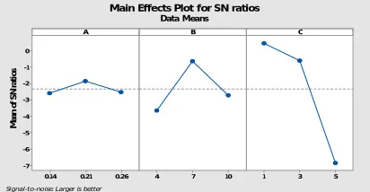
According to Taguchi philosophy the use of loss function to measure the deviation between the experimental value and the desired value which is further transformed into signal-to-noise ratio (S/N). Basically, there are three types of categories in the evaluation of signal-to-noise ratio i.e.

Lower-the-better (LB), higher-the-better (HB) and nominal- the-better (NB) .The objective of paper is to optimize the process parameter for MRR, over cut and for finding MRR higher the better has been taken to calculate the singal to noice ratio .and lower-the-better characteristic has been taken to calculate the other response parameter.

The optimal parameters were chosen based on higher S/N ratio as signal represents desirable value and noise represents undesirable value. Next, statistical analysis of variance (ANOVA) was conducted to study the significance of process parameters on responses based on their P-value and F-value at 95% confidence level.

0.26 0.21 0.14 1.3 1.2 1.1 1.0 0.9 0.8 0.7 0.6 0.5 0.4 10 7

4 1 3 5

A M ea n o f M e an s B C

Main Effects Plot for Means

Data Means 0.26 0.21 0.14 0 -1 -2 -3 -4 -5 -6 -7 10 7

4 1 3 5

A M ea n o f S N r a ti o s B C

Main Effects Plot for SN ratios

Data Means

Signal-to-noise: Larger is better

Fig 6.1 main effect plot MRR for means (W) Fig 6.2 main effect plot MRR for SN Ratio (W)

B A 10 9 8 7 6 5 4 0.250 0.225 0.200 0.175 0.150 > – – – – – – < 0.5 0 0.5 0 0.75 0.75 1.0 0 1.0 0 1.2 5 1.2 5 1.5 0 1.5 0 1.75 1.75 2.0 0 2.0 0 MRR

Contour Plot of MRR vs A, B

C B 5 4 3 2 1 10 9 8 7 6 5 4 > – – – – – – < 0.50 0.50 0.75 0.75 1.00 1.00 1.25 1.25 1.50 1.50 1.75 1.75 2.00 2.00 MRR

A. Contour plot of MRR vs A, B

In the above figure show the dark blue region is lower metal removal rate and then increasing with light blue so we can say that parameter B from 4 to 6 and parameter A from 0.15 to 0.25 cover small MRR as compare to other region of contour plot.

B. Contour plot of MRR vs B, C

In the above figure show the dark green region is higher metal removal rate and then decreasing with light blue and blue so we can say that parameter B from 5 to 8.5 and parameter C from 1 to 3 cover large MRR as compare to other region of contour plot.

C B 5 4 3 2 1 10 9 8 7 6 5 4 > – – – – – – < 1 1 2 2 3 3 4 4 5 5 6 6 7 7 OVERCUT

Contour Plot of OVERCUT vs B, C

B A 10 9 8 7 6 5 4 0.250 0.225 0.200 0.175 0.150 > – – – – – – < 1 1 2 2 3 3 4 4 5 5 6 6 7 7 OVERCUT

Contour Plot of OVERCUT vs A, B

Fig contour plot of OVERCUT vs B, C Fig contour plot of OVERCUT vs A, B

0.25 5 . 0 0 2 . 0 1.0 1.5 4 2.0

6 0 15.

8 0 1 R R M A B B , A s v R R M f o t o l P e c a f r u S 0.25 0 0 .

0 0.2

2.5 5.0

4 7.5

6 0 5.1

8 0 1 T U C R E V O A B B , A s v T U C R E V O f o t o l P e c a f r u S

Fig surface plot of overcut VS A,B (NB) Fig surface plot of overcut VS A, B (NB)

VI.CONCLUSION

The experimental results for optimal settings showed that there was a considerable improvement in the performance characteristics viz., MRR and OC. And using grey technique the optimal parameter of input is A2 B2 AND C1 and the value of MRR and OC is 2.23222.0621(mg/min) and 1.2112(mg/min) respectively for W. and apart from that the optimal result in the case of NB the percentage of SiC in ZrB2 is 14 percentages is the optimum and pulse on time is 7 μs and pulse off time is 1 μs. For this input

REFERENCES

[1] Mukherjee I, Ray PK. A review of optimization technique in metal cutting process, Computer & Industrial Engg 2006; 50: 15-34.

[2] Kao PS, Hocheng H. Optimization of electrochemical polishing of stainless steel by grey relational analysis. j mater proesstechnol 2003;140:255-9

[3] Chiang KT, Chang FP. Optimization of the WEDM process of particle-reinforced material with multiple performance characteristics using grey relational analysis. J Mater Process Technol 2006; 180:96

[4] Monteverde F, Bellosi A , Luigi Scatteia. Processing and properties of ultra-high temperature ceramics for space applications. Mater SciEngg A 2008; 485:

415–21

[5] Wen KT, Chang TC, You ML. The grey entropy and its application in weighting analysis. IEEE International Conference on Systems, Man, and Cybernetics 1998; 2:1842–4.

[6] Chiang YM, Hsieh HH. The use of the Taguchi method with grey relational analysis to optimize the thin-film sputtering process with multiple quality characteristics in colour filter manufacturing. Computer and Industrial Engg 2009; 56:648–61.

[7] Hewidy MS, El-Taweel TA, El-Safty MF. Modelling the machining parameters of wire electrical discharge machining of Inconel 601 using RSM. J Mater

Process Technol2005 ; 169: 328–36.

[8] Puertas I, Luis CJ, Álvarez A. Analysis of the influence of EDM parameters on surface quality, MRR and EW of WC–Co. J Mater Proces. Technol2004;153–

154: 1026–32.

[9] George PM, Raghunath BK, Manocha LM, Warrier A.M.EDM machining of carbon–carbon composite—a Taguchi approach. J Mater Process Technol 2004;

145: 66-71.

[10] Mahdavinejad R.A(2009) EDM process optimization via predicting a controller model, International Scientific Journal published quarterly by the Association of Computational Materials Science and Surface Engineering,1( 3):161-167

[11] In-Jun Jeong a, Kwang-Jae Kim(2009) An interactive desirability function method to multiresponse optimization, European Journal of Operational Research

195:412–426

[12] Surajit Pal a, Susanta Kumar Gauri(2010) Assessing effectiveness of the various performance metrics for multi-responseoptimization using multiple regression,

Computers & Industrial Engineering 59: 976–985

[13] AmanAggarwal, Hari Singh, Pradeep Kumar, Manmohan Singh(2008)Optimization of multiple quality characteristics for CNCturning under cryogenic cutting

environment using desirability function,journal of materials processing technology 205:42–50

[14] Indrajit Mukherjee, Pradip Kumar Ray (2008)Optimal process design of two-stage multiple responses grindingprocesses using desirability functions and metaheuristictechnique,Applied Soft Computing 8: 402–421

[15] AysunSagbas(2011) Analysis and optimization of surface roughness in the ball burnishing processusing response surface methodology and desirabilty

function,Advances in Engineering Software 42 :992–998

[16] F. George, Luger A. William, Stubblefield, The Benjamin Cummings Publishing Company, Inc., 1993.

[17] N. Tosun, L. Ozler, J. Mater. Process. Technol. 124 (2002) 99–104.

[18] E.M. Bezerra, A.C. Ancelotti, L.C. Pardini, J.A.F.F. Rocco, K. Iha, C.H.C. Ribeiro, Mater. Eng. A 464 (2007) 177–183.

[19] W.C. Chen, G.L. Fu, P.H. Tai, W.J. Deng, Exp. Syst. Appl. 36 (2009) 1114–1122.

[20] J. Zhixin, Z. JianhuaA. Xing(1995), Ultrasonic vibration pulse electrodischarge machining of holes in engineeringceramics, Journal of Materials Processing

Technology

[21] S. M. Metev and V. P. Veiko, Laser Assisted Microtechnology, 2nd ed., R. M. Osgood, Jr., Ed. Berlin, Germany: Springer-Verlag, 1998.

[22] J. Breckling, Ed., The Analysis of Directional Time Series: Applications to Wind Speed and Direction, ser. Lecture Notes in Statistics. Berlin, Germany: Springer, 1989, vol. 61.

[23] S. Zhang, C. Zhu, J. K. O. Sin, and P. K. T. Mok, “A novel ultrathin elevated channel low-temperature poly-Si TFT,” IEEE Electron Device Lett., vol. 20, pp.

569–571, Nov. 1999.

[24] M. Wegmuller, J. P. von der Weid, P. Oberson, and N. Gisin, “High resolution fiber distributed measurements with coherent OFDR,” in Proc. ECOC’00, 2000,

paper 11.3.4, p. 109.

[25] R. E. Sorace, V. S. Reinhardt, and S. A. Vaughn, “High-speed digital-to-RF converter,” U.S. Patent 5 668 842, Sept. 16, 1997.

[26] (2002) The IEEE website. [Online]. Available: http://www.ieee.org/

[27] M. Shell. (2002) IEEEtran homepage on CTAN. [Online]. Available: http://www.ctan.org/tex-archive/macros/latex/contrib/supported/IEEEtran/

[28] FLEXChip Signal Processor (MC68175/D), Motorola, 1996.

[29] “PDCA12-70 data sheet,” Opto Speed SA, Mezzovico, Switzerland.

[30] A. Karnik, “Performance of TCP congestion control with rate feedback: TCP/ABR and rate adaptive TCP/IP,” M. Eng. thesis, Indian Institute of Science,

Bangalore, India, Jan. 1999.

[31] J. Padhye, V. Firoiu, and D. Towsley, “A stochastic model of TCP Reno congestion avoidance and control,” Univ. of Massachusetts, Amherst, MA, CMPSCI

Tech. Rep. 99-02, 1999.