RESEARCH LETTER
MST radar signal processing using
iterative adaptive approach
C. Raju
*†and T. Sreenivasulu Reddy
†Abstract
Power spectrum is the considerable aspect in the atmospheric radar data processing to estimate wind parameters. Due to the poor resolution and high sidelobe level problems of the existing algorithms, there is a requisite for the novel data-dependent approaches. A non-parametric and hyperparameter-free iterative adaptive approach (IAA) is presented for the power spectral density estimation. This approach is able to work with single snapshot and is obtained by minimizing the weighted least square fitting criterion. The IAA method provides the accurate amplitude and frequency estimation for the simulated data. The data for the above study is collected from Indian MST (meso-sphere, strato(meso-sphere, and troposphere) radar. The power spectrum and Doppler frequency are estimated using IAA. In this paper, zonal (U), meridional (V), windspeed (W) are also calculated and validated using Global Positioning System Sonde data. The effectiveness of the spectral estimation performance showed by IAA is demonstrated and assessed.
Keywords: Spectral estimation, MST radar, IAA, GPS
© The Author(s) 2018. This article is distributed under the terms of the Creative Commons Attribution 4.0 International License (http://creat iveco mmons .org/licen ses/by/4.0/), which permits unrestricted use, distribution, and reproduction in any medium, provided you give appropriate credit to the original author(s) and the source, provide a link to the Creative Commons license, and indicate if changes were made.
Background
Indian MST radar provides information on wind data above 3.5 km with a resolution of 150 m. The three wind components U, V and W are determined by the Doppler beam swinging (DBS) method of the MST radar. The radar collects the data using multiple beam positions with 16 μs coded pulse and with an inter pulse period (IPP) of 100 μs. The online calculation of Doppler power spectra for each range bin can be obtained by subjecting the complex time series data to the process of fast Fourier transform (FFT). The DC removal, average noise level estimation, interference removal and incoherent integra-tion are the steps that are involved in offline data process-ing. The 0th, 1st and 2nd moments denotes the signal strength, mean Doppler shift and half width parameters of the spectrum are computed, respectively.
The accurate estimation of the Doppler frequency is the crucial one in the detection and estimation of the wind speed by the MST radar. A package for process-ing the radar data has been developed by the National
Atmospheric Research Laboratory (NARL), Gadanki, Andhra Pradesh, India. It is known as the atmospheric data processor (ADP) (Anandan 2002). The Doppler fre-quencies can be accurately estimated by the ADP up to certain heights. Since the signals are highly corrupted with noise at higher altitudes, the ADP is unable to esti-mate the Doppler frequencies and thus the wind speed. It can be seen in the literature that several algorithms have been put to use to accurately estimate the Doppler fre-quencies from MST radar data.
Bispectral estimation algorithm (Anandan et al. 2001) is applied to radar at a high computational cost. The multitaper-based spectral estimation (Anandan et al.
2004) has the advantage of reduction in variance and has been applied to the radar data. However, it has spectral peak broadening. An adaptive estimation technique has been presented to estimate the Doppler spectra, with certain parameters to adaptively track the signal in the range of Doppler spectral frame (Anandan et al. 2005). Several methods like wavelet-based denoising (Thati-parthi et al. 2009) and cepstral thresholding (Reddy and Reddy 2010a, b) have also been used for spectrum clean-ing and then Doppler spectrum estimation leadclean-ing to the calculation of wind velocities. According to (Reddy and Reddy 2010a, b), a polyphase approach was employed for
Open Access
*Correspondence: [email protected]
spectrum estimation using uniform filter banks. Recent studies applied principal component analysis (PCA) on the radar data, prior to periodogram estimation using Blackman–Tukey, and minimum variance methods (Uma Maheswara Rao et al. 2014). All the existing methods used in spectral estimation for atmospheric radar data falls under two estimation methods either parametric or nonparametric. However, parametric method requires the prior knowledge of some parameters and nonpara-metric method has global leakage (peaks at unwanted frequencies) and local leakage (main beam limits). In the present study, the iterative adaptive approach (IAA) (Yardibi et al. 2010) is put into use to estimate the spec-trum of MST radar data collected from NARL. The IAA algorithm is based on weighted least squares minimiza-tion and is found to give excellent results for simulated data and real-time data.
In this paper, lowercase and uppercase boldface letters represent vectors and matrices, respectively. Normal let-ters are used to indicate scalar quantities. Notations | · | ,
�·� , (·)∗ , (·)T , and E(·) denote the modulus, the Frobe-nius norm, the complex conjugate transpose (Hermitian transpose), the transpose and the expectation operator. Subscript [·]k denotes the kth element of a vector, and IN represents an identity matrix of size N.
Data model
The MST radar data collected from the NARL is a uni-formly spaced complex baseband signal consisting of in-phase (I) and quadrature (Q) phase components.
Let
yn
N
n=1 be the complex data obtained by weighted combination of C complex exponentials with frequencies {Ωr}Nr=1∈[0,Ωmax]
where C is a small number, {tn}Nn=1 denotes the sampling time instants which can be non-uniformly spaced. qr is the magnitude associated with r-th frequency compo-nent Ωr, en is the additive white Gaussian noise compo-nent corresponding to the n-th sampling time.
Consequently, the complex data signal can be modelled as
The expanded version of the above equation is
(1) yn=
C
r=1
qrejωrtn+en
(2)
yn= R
r=1
qrejωrtn+en
(3) y1 .. . yN =
ejω1t1 · · · ejωRt1
..
. . . . ... ejω1tN · · · ejωRtN
q1 .. . qR + e1 .. . eN
Those values of r for which ωr∈ {Ωr}Nr=1 , the corre-sponding qr values will be non-zero. The equation can vectorially be represented in the following form:
where y=[y1,y2,. . .,yN]T,D=[d(ω1),d(ω2),. . .,d(ωN)]T with
q=[q1,q2,. . .,qR]T , |qr|2 is the power value associ-ated with the r-th frequency component that has to be estimated.
Iterative adaptive approach
Iterative adaptive approach is a weighted least square-based data-dependent, non parametric algorithm. It can be used for the single data sequence or the multiple data snapshots spectral estimation. Here, we assume the sin-gle snapshot case.
The covariance matrix of the received signal is given by the following model
where
where {mi}Ri=+1N is a replacement for
|qi|2R +N
i=1 . The first
R diagonal elements of the matrix P denote the power values that are to be estimated and the remaining N diag-onal elements denote the noise variance values.
The IAA algorithm is based on the minimization of weighted least squares fitting criterion,
where �X�2
O−r1 X
HO−1
r X.Or is the interference covari-ance matrix written as
Let mr(i) denotes the estimate of mr at ith iteration, and let R(i) be the covariance matrix R derived from{mi}Ri=+1N.
Minimizing the Eq. (9) with respect to mr,r=1, 2,. . .,R+N, yields
(4) y=Dq+e
(5) d(ωr)=
ejω1t1,. . .,ejωrtN
=dr
(6)
R=E
yy∗
= R
r=1
|qr|2drd∗r +E
ee∗
=DPD∗
(7)
E ee∗
=diag(σ1,σ2,. . .,σN)
(8) P=diag|q1|2,|q2|2,. . .,|qR|2,σ1,σ2,. . .,σN
diag(m1,m2,. . .,mR+N)
(9)
f =y−drmr
2
O−r1, r=1, 2,. . .,R+N
(10) Or =E
Making use of the Woodbury matrix identity of
The estimation of the power by means of the following iterative process
The initial estimate mr(0) can be obtained using the single frequency least-squares (SFLS) method (which is known as periodogram).
The algorithm is summarized in Table 1.
Results Simulation
The simulation results for the complex data explained in Data Model are displayed. With N = 200 and C = 3, the data samples are generated from a signal consisting of three exponentials at 0.3100, 0.3150, 0.1450 Hz frequen-cies having the amplitudes q1=10ejϕ1,q2=10ejϕ2, and
q3=10ejϕ3 with a sampling interval of 1 s. The phase values {ϕr}3r=1 are distributed in uniform and
independ-ent manner [0, 2π]. The noise component is introduced in the ɛ term, which is the normal white noise with zero mean and σ variance. The signal-to-noise ratio (SNR) in dB for the data model is defined as SNR=10 log100σ .
The power spectrum of the original test signal gener-ated using the data model before adding noise is depicted in Fig. 1. The spectrum of the signal for SNR = 0 dB using periodogram and IAA are shown in Fig. 2. The peri-odogram is obtained by padding the 200 element time-series data with 312 zeros and performing the 512-point FFT. For IAA the number of processing points R is taken as 512.
(11)
ˆ
mr(i+1)=
d∗rO−r1y d∗
rO−r1dr
, r=1, 2,. . .,R+N
(12)
d∗rO−1r = d ∗
rR−1(i)
1− |mr(i)|d∗rR−1(i)dr
(13) ˆ
mr(i+1)=
d∗rR−1(i)y d∗
rR−1(i)dr
, r=1, 2,. . .,R+N
(14)
mr(0)=
d∗ry
2
�dr�4
, r=1, 2,. . .,R+N.
Table 1 Summary of the IAA algorithm
S. no. Operation
1. Initialize the value mr(0) using the periodogram
2. Compute the covariance matrix R=R+N
r=1 mrdrd∗r
3. Update mˆr(i+1) using the equation for r=1, 2,. . .,R+N
4. Repeat steps 2–3 until the convergence condition is reached
Fig. 1 Spectrum of the original signal
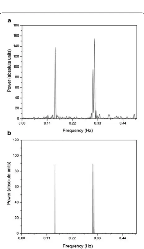
Fig. 2 Spectrum of the test signal for SNR = 0 dB a periodogram b
The root mean square error (RMSE) of the frequency estimation and amplitude estimation versus SNR plots are shown in Fig. 3a, b, respectively. All the performance curves are obtained via 100 Monte Carlo simulations. We change the value of σ2 to obtain different signal-to-noise ratio conditions. From Fig. 3a, b, it can be observed that both the RMSE of the frequency and the amplitude esti-mates decreased with the SNR as expected. It can also be observed that the IAA method has better variance char-acteristics than the Periodogram method. It is evident
from the above simulations, that even the signal is com-pletely buried in noise the IAA method is able to retrieve the parameters well.
MST radar data
The radar data collected from the Indian MST radar being operated at the NARL, Gadanki, Andhra Pradesh is taken for the present study. The MST radar data is one of the e formats of 15 scans with each scan having sig-nal information from six beam directions (East, West, Zenith-X, Zenith-Y, North and South). Each beam con-sists of 147 height range bins with a resolution of 150 m, starting from 3.6 km and reaching to a height of 25.6 km. Each range bin contains complex time-series data with 512 samples. The spectrum of the radar signal is calcu-lated using IAA. Since, the echoes are usually corrupted by interference, clutter, etc., it has to be cleaned before analysis. Maximum peak detection method (Anandan et al. 1996) is used for the estimation of Doppler profile after performing spectrum cleaning of the radar signal. The Doppler frequencies are calculated from the Doppler profiles.
Once the Doppler frequencies are computed, the Dop-pler velocities are found out by multiplying each of the frequencies with c/2fc where c is the velocity of light and
fc is the operating frequency of the Doppler radar. Both Doppler frequencies and the velocities are calculated for all 6 beams and 147 range bins. Using the Doppler veloci-ties for the 6 beams denoted as vE,vW,vZX,vZY,vN,vS
where the subscripts represents the corresponding beams, the three wind velocities components are evalu-ated as follows
where vx, vy, vz are the zonal U, meridional V, and the ver-tical Z velocity components. The Zenith-X and Zenith-Y beams are in the vertical direction and do not play a role in the determination of the wind velocity.The Wind speed
W is computed as
(15)
vx vy vz
=
0.603 0 0
0 0.603 0
0 0 0.603
−1
∗
0.1736(vE−vW) 0.1736(vN−vS) 0.1736(vZX−vZY)
(16) W =v2x+v2y
1/2 Fig. 3 a RMSE of normalized frequency versus SNR. b Amplitude
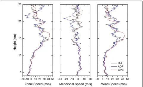
The wind speed thus obtained is then compared with the corresponding wind speed collected from the global positioning system (GPS) radiosonde (Jagannadha Rao et al. 2003).
The power spectrum of the collected data is deter-mined using IAA method. The basic method of peri-odogram is employed for estimating the power spectrum when complex time-series data is subjected to the ADP.
Figure 4a, b shows the improvement of output SNR estimated from power spectrum using periodogram and IAA for the east and south beams, respectively, for the MST radar data collected on February 9, 2015. The out-put SNR is obtained using the method (Hildebrand and Sekhon 1974). The comparison of average SNR values in dB for six beams on February 9 and 10, 2015 for the peri-odogram and IAA algorithms is given in Table 2. From Fig. 4 Height profiles of SNR estimated using periodogram and IAA. a East beam; b south beam for data collected on February 9, 2015
Table 2 Comparison of average SNR for periodogram and IAA algorithm
Date Algorithm East West North South Zenith-X Zenith-Y
Feb 9, 2015 Periodogram 19.47 18.23 20.14 21.57 18.45 17.98
IAA 23.84 22.48 22.65 24.09 22.84 21.45
Feb 10, 2015 Periodogram 22.35 23.41 18.56 17.86 20.85 19.81
Table 2, it is seen that the IAA gives the better improve-ment in SNR values for all the six beams.
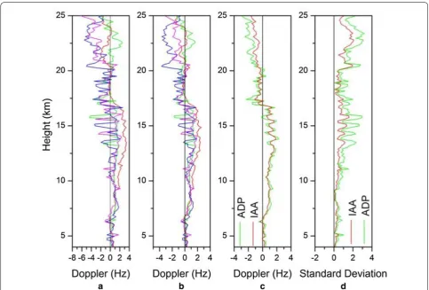
The Doppler height profiles for four scans of the east beam attained using ADP and IAA are shown in Fig. 5a, b, respectively, for the radar data collected on February 9, 2015. The compared mean Doppler profiles and stand-ard deviations are shown in Fig. 5c, d respectively. The observed significant difference between ADP and IAA is that the standard deviation for IAA lied very close to zero.
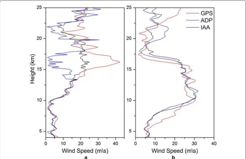
drift of the balloon due to high wind speeds. The wind speeds using ADP, IAA and GPS radiosonde for real-time radar data collected on two different dates namely July 2, 2014 and February 9, 2015 is represented in Fig. 8.
The consistency of the algorithm is checked by calcu-lating the correlation between GPS radiosonde data and IAA wind speeds for the radar data collected during 4th–8th October, 2006 and 9th–12th February, 2015. A significant correlation coefficient of 0.8996 and 0.9246 is obtained between the GPS and IAA, 0.843 and 0.85406 between GPS and ADP, respectively. The high correlation
factor acquired is indicating the relative accuracy of the wind speed calculated using IAA method confirming its efficiency and effectiveness. Figures 9 and 10 shows the correlation between IAA and GPS wind speeds.
Conclusion
proves that IAA functions superior compared to existing algorithms which have failed to perform well especially in this height range. Significant enhancement in SNR at higher altitudes is achieved with IAA demonstrating its efficiency and effectiveness. The obtained wind veloci-ties from the IAA algorithm are validated using the GPS sonde values. The correlation between wind speeds
Fig. 8 Wind speed using ADP, IAA and GPS radiosonde for radar data collected on a July 2, 2014 b February 9, 2015—Comparison
Fig. 9 Correlation between IAA and GPS wind speeds for data during 4th–8th October 2006
methods which results in consuming less computational time.
Authors’ contributions
Both authors read and approved the final manuscript.
Acknowledgements
The authors would like to thank National Atmospheric Research Laboratory (NARL), Gadanki for providing radar data and Centre of Excellence, Depart-ment of Electronics and Communication Engineering, Sri Venkateswara University College of Engineering for technical assistance.
Competing interests
The authors declare that they have no competing interests.
Availability of data and materials
The data is archived at the National Atmospheric Research Laboratory, Gadanki, India.
Funding
Not applicable.
Publisher’s Note
Springer Nature remains neutral with regard to jurisdictional claims in pub-lished maps and institutional affiliations.
Received: 1 June 2018 Accepted: 2 August 2018
References
Anandan VK (2002) Atmospheric data processor-technical and user reference manual. NMRF, DOS Publication, Gadanki
Anandan VK, Balamuralidhar P, Rao PB, Jain AR (1996) A method for adap-tive moments estimation technique applied to MST radar echoes. In: Proceedings of the Progress Electromagnetics Research Symposium, pp 360–365
Anandan VK, Reddy GR, Rao P (2001) Spectral analysis of atmospheric radar signal using higher order spectral estimation technique. IEEE Trans Geosci Remote Sens 39(9):1890–1895
Anandan VK, Pan C, Rajalakshmi T, Reddy GR (2004) Multitaper spectral analysis of atmospheric radar signals. Ann Geophys 22(11):3995–4003
Anandan VK, Balamuralidhar P, Rao P, Jain A (2005) An adaptive moments esti-mation technique applied to MST radar echoes. J Atmos Ocean Technol 22:396–408
Hildebrand PH, Sekhon R (1974) Objective determination of the noise level in Doppler spectra. J Appl Meteorol 13(7):808–811
Jagannadha Rao VVM, Narayana Rao D, Venkat Ratnam M, Mohan K, Vijaya Bhaskar Rao S (2003) Mean vertical velocities measured by Indian MST radar and comparison with indirectly computed values. J Appl Meteorol 42(4):541–552
Reddy TS, Reddy GR (2010a) MST radar signal processing using cepstral Thresholding. IEEE Trans Geosci Remote Sens 48(6):2704–2710 Reddy TS, Reddy GR (2010b) Spectral analysis of atmospheric radar
sig-nal using filter banks polyphase approach. Digit Sigsig-nal Process 20(4):1061–1071
Thatiparthi S, Gudheti R, Sourirajan V (2009) MST radar signal processing using wavelet-based denoising. IEEE Geosci Remote Sens Lett 6(4):752–756 Uma Maheswara Rao D, Reddy TS, Reddy GR (2014) Atmospheric radar signal
processing using principal component analysis. Digit Signal Process 32:79–84