LED-based Vis-NIR spectrally tunable light source - the optimization algorithm

R E S E A R C H

Open Access

LED-based Vis-NIR spectrally tunable light

source - the optimization algorithm

M. Lukovic

, V. Lukovic

, I. Belca

, B. Kasalica

, I. Stanimirovic

and M. Vicic

Abstract

Background:A novel numerical method for calculating the contributions of individual diodes in a set of light emitting diodes (LEDs), aimed at simulating a blackbody radiation source, is examined. The intended purpose of the light source is to enable calibration of various types of optical sensors, particularly optical radiation pyrometers in the spectral range from 700 nm to 1070 nm.

Results:This numerical method is used to determine and optimize the intensity coefficients of individual LEDs that contribute to the overall spectral distribution. The method was proven for known spectral distributions:“flat” spectrum, International Commission on Illumination (CIE) standard daylight illuminant D65 spectrum, Hydrargyrum Medium-arc Iodide (HMI) High Intensity Discharge (HID) lamp, and finally blackbody radiation spectra at various temperatures.

Conclusions:The method enables achieving a broad range of continuous spectral distributions and compares favorably with other methods proposed in the literature.

Keywords:Algorithmic solution, LEDs, Calibration source, Blackbody, Optical pyrometers

Background

Numerous variants of spectral light sources based on com-bined radiation of individual LEDs have been reported in the past 15 years [1–4]. Each LED has its own spectral char-acteristic and contributes to the overall output spectrum in a relatively narrow range. As the number of newly-developed semiconductor light sources increases, covering wider and wider spectral range, this kind of construction be-comes increasingly popular [5–7]. This approach allows for the generating a broad range of different output spectral dis-tributions of almost arbitrary shape. This in turn, enables various applications such as calibration of light-measuring instruments, ambient lighting, applications in forensic sci-ence, fluorescence applications [8–10], etc.

Special case of light sources based on combined emis-sion from a set of LEDs (where each individual LED has its own spectral distribution) are calibration sources [11–17]. Such instruments often allow for the generation of arbitrary shaped output spectrum. For example, refer-ence [9] describes a LED-based calibration source for an ultra-sensitive spectrometry system used for electro- and

photo-luminescent measurements. However, extensive search through available literature produced only a few readily implementable prescriptions for synthesizing the output spectrum of a LED-based tunable source [15, 17]. The objective of this paper is to explore the possibilities for improving spectrum synthesis methods.

We explore the possibilities of generating various spectral shapes in the very near infrared region (VNIR) using a relatively large number of individual LEDs. It is our belief that the results of this work might be useful to other researchers in this field.

Special emphasis will be placed on generating a simulated

“flat”spectrum and blackbody radiation spectra in the 700 -1070 nm range for the 800 - 1300 °C temperature interval. However, the proposed methodology should be readily ap-plicable to other spectral ranges and/or temperatures [18].

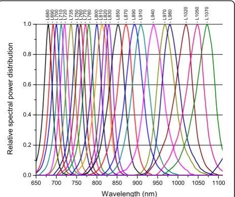
The basic problem of synthesizing the shape of a given spectral profile is determining the intensity of each indi-vidual LED that contributes to the overall spectrum. Each LED has a relatively narrow spectral distribution as illustrated in Fig. 1 [19]. In the first approximation, the spectral distribution of a single LED will be assumed to be Gaussian. The synthesized output spectrum is a sum of the contributions from each individual LED’s

* Correspondence:[email protected]

1_{University of Kragujevac, Faculty of Technical Sciences, Cacak 32000, Serbia}

Full list of author information is available at the end of the article

normalized spectral power distribution (SPD) weighted by a certain factor. This factor in fact corresponds to the current that drives the particular LED, in order to get unity intensity at Gaussian center.

For a given target output spectral profile, it is therefore necessary to mathematically find the combination of values of the coefficients (driving current intensities) that best iterate the target spectrum. An algorithmic solution was developed to achieve this.

The algorithm was initially applied for the synthesis of a flat spectrum, i.e. for producing an output spectrum that has a constant intensity with respect to the wavelength in the given wavelength interval. The“flat”spectrum can be an excellent tool for direct measurements and evaluation of the responsivity function of optical sensors and systems like low-signal intensity measuring spectrometers, photo-multipliers, etc., where standard lamps and black bodies introduce large relative errors due to a great intensity vari-ation (almost two orders of magnitude).

A further refinement of the algorithm was used to synthesize arbitrarily shaped spectrum profiles and in particular to simulate blackbody radiation. Deviation of the synthesized blackbody spectra from the theoretical curve was analyzed in detail. This was done in order to estimate the temperature reading errors when the LED-based source is used as a calibration source for optical pyrometers. A LED-based system that simulates black-body radiation would be a handy and practical solution for calibrating pyrometers in industrial installations, opposite to large blackbody furnaces.

Methods

As already mentioned, the main purpose of the proposed algorithm for a given number of LEDs is to find the coefficients (weight factors) that multiply the driving

currents of a LED in such way that the summary output spectral profile represents the best possible approxima-tion of the desired output spectral profile.

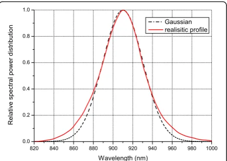
In order to simplify calculations, we assumed that the SPDs of individual LEDs are normalized. In other words, the output intensity for the emission peak of each LED has a unity value. One has to bear in mind that in prac-tical implementations LEDs feature different emission efficiencies. Therefore, the coefficients obtained through simulation need to be multiplied by an appropriate fac-tor that accounts for different LED efficiencies.

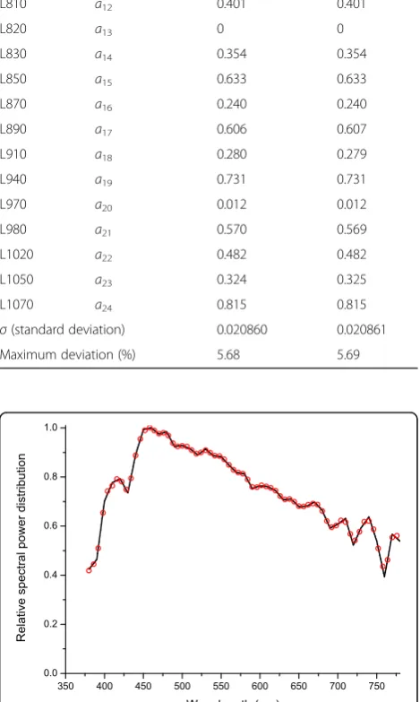
Table 1 shows the relative light intensity emitted by in-dividual LEDs per unit current (i.e. emission gain) in the wavelength interval 632-1548 nm. The LEDs used were: L680, L690, L700, L710, L720, L735, L750, L760, L770, L780, L800, L810, L820, L830, L850, L870, L890, L910, L940, L970, L980, L1020, L1050, L1070, L1200, L1300, L1450 and L1550. The labels and the intensity data were adopted from [19]. Figure 2 illustrates the typical SPD of a diode from the set (L910 in this example).

Determining the values of the sought coefficients in linear algebra comes down to solving m equations with

n unknown coefficients aj (j= 1,…n) according to (1), Fig. 1Relative SPDs of different LEDs in the spectral range 650 - 1110 nm

Table 1Matrix M of relative LED SPDs in the spectral range from 632 nm to 1548 nm with an increment of 4 nm. LEDs: L680, L690,…, L1550

Wavelength (nm)

LED

L680 L690 L700 … L1450 L1550

632 0.006757 0 0 … 0 0

636 0.013514 0 0 … 0 0

640 0.027027 0 0 … 0 0

644 0.041892 0.006757 0 … 0 0

648 0.067568 0.013514 0.006757 … 0 0

652 0.108108 0.027027 0.02027 … 0 0

656 0.151351 0.041892 0.02973 … 0 0

660 0.22973 0.067568 0.040541 … 0 0

664 0.337838 0.108108 0.060811 … 0 0

668 0.486486 0.151351 0.090541 … 0 0

672 0.689189 0.22973 0.135135 … 0 0

676 0.891892 0.337838 0.189189 … 0 0

680 1 0.486486 0.27027 … 0 0

684 0.891892 0.689189 0.364865 … 0 0

688 0.689189 0.891892 0.5 … 0 0

692 0.445946 1 0.702703 … 0 0

696 0.27027 0.891892 0.905405 … 0 0

700 0.175676 0.689189 1 … 0 0

… … … …

1544 0 0 0 … 0.040541 0.986486

whereM represents the matrix of relative SPDs derived from Table 1, depending on the number of chosen diodes

nand the selected spectral bandwidthm.

a1M11þa2M12þ…þanM1n ¼ I1

a1M21þa2M22þ…þanM2n ¼ I2

…

a1Mm1þa2Mm2þ…þanMmn¼Im

ð1Þ

The matrix form of (1) is given in (2) and (3), whereA represents a matrix of unknown LED coefficients and I represent a matrix of targeted intensities. The element

Mijof the matrixMrepresents the spectral contribution on the i-th wavelength of the j-th LED. The matrix M has the dimensions m×n with non-zero elements mainly concentrated along its diagonal. Owing to the fact that m>n, mathematical problem (1) is actually an overdetermined system.

M11M12…M1n M21M22…M2n

… Mm1Mm2…Mmn 2 6 6 6 6 4 3 7 7 7 7 5 a1 a2 … an 2 6 6 4 3 7 7 5¼ I1 I2 … Im 2 6 6 4 3 7 7

5 ð2Þ

M¼

M11M12…M1n

M21M22…M2n … Mm1Mm2…Mmn 2 6 6 6 6 6 4 3 7 7 7 7 7 5; A¼

a1 a2 … an 2 6 6 4 3 7 7 5; I¼

I1 I2 … Im 2 6 6 4 3 7 7 5

ð3Þ

The optimal solution to this kind of problem can be sought by several different methods (e.g. see [20–24]).

We proposed yet another innovative approach, starting from the following assumptions:

The target spectral profile is well-defined.

The interval of the simulated wavelengths is covered bynLED sources.

Each LED’s SPD can be initially approximated by a Gaussian, to accelerate calculations. However, final calculations are performed using real SPDs. The contribution of each LED to the summary

spectrum is determined by a coefficientaj(j= 1,…n), which is proportional to the driving current of that LED.

All coefficientsa_jmust be in the intervallb_a<a_j<ub_a. The values of the lowerlbaand the upperubainterval boundary depend on the shape of the target.

The system of Eq. (1) in the new approach is solved by allowing for the summed intensities I1, I2, …,Im to

slightly deviate from the prescribed values of the target intensities IT1, IT2, …,ITm. The coefficients a1, a2,.., an

are varied within their expected range and for each vari-ation a standard devivari-ation from the target intensitiesIT1, IT2, …,ITm is calculated and stored. This procedure

en-ables finding of the variation of coefficientsa1,a2,…,an

that yields the minimum deviation of the combined LEDs spectral distribution from the target SPD. The out-line of the proposed optimization algorithm is presented in the flowchart shown in Fig. 3.

Each coefficient aj is determined with resolution res,

which gives a number of possible values for eachajas:

N¼ðuba−lbaÞ=res ð4Þ

Under these assumptions, it is possible to generate Vr

different spectra (variations with repetition):

V r¼Nn ð5Þ

The criterion for selecting the best variation is min-imal standard deviation from the target SPD. Taking into account the spectral range in which optical pyrometers would operate and the purpose for which it would be used, the spectral interval of interest in our research was 700 - 1070 nm. Choosing of the best values for the coef-ficientsa1,a2,..,anby finding the variation that produces

the minimum deviation of the synthesized spectrum in mentioned spectral region, was limited by the availability of LEDs on the market. Due to this constraint, we cov-ered the interval by n= 24 LED models: L680, L690, L700, L710, L720, L735, L750, L760, L770, L780, L800, L810, L820, L830, L850, L870, L890, L910, L940, L970, L980, L1020, L1050 and L1070. To broaden the dynamic range, a group of four identical devices were used for each diode model. Since we wished to determine the

coefficients accurately to the third decimal place (res= 0.001), according to (4) it followed that N= 4000. Based on (5), for 24 LED models the overall number of varia-tions was Vr= 400024. The number of variations repre-sented a formidable computing challenge and it was necessary to further reduce it. This was achieved by: (i) reducing the number of possible coefficient values and (ii) reducing the number of diodes that were simultan-eously active during the optimization run.

The number of possible coefficient values was reduced by an iterative procedure, where N= 3 was kept fixed, while the interval and the resolution were simultan-eously decremented.

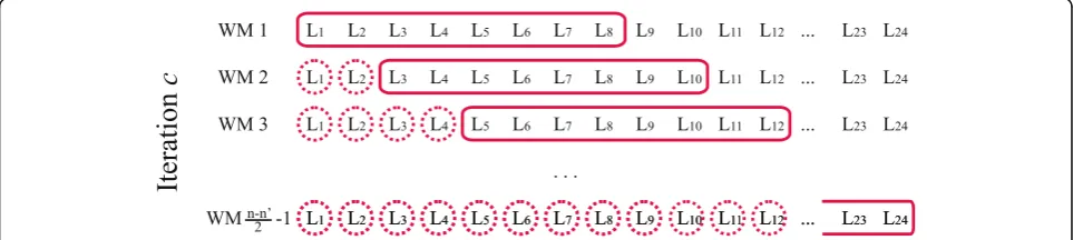
The reduction in the number of active diodes during optimization was effectively achieved by shortening the wavelength interval for the optimization search. This

procedure started by taking the first n'diodes (arranged by increasing wavelength). The numbern'was chosen so that computer optimization over the shortened wave-length interval could be carried out in a reasonable time. The next step involved shifting of the “optimization window” by two spaces to the right. Thus, a new set on

n' diodes underwent an optimization run. The coeffi-cients left of the current window remained as calculated in the previous run. The procedure was repeated until the optimization window reached the rightmost diode (the diode with the longest wavelength). Figure 4 is a graphical representation of the procedure.

The search for the coefficients in the optimization window was performed using the following method: three values (_N= 3) of the coefficients were evaluated for each iteration step and each diode. In the first

Fig. 3Flowchart of the proposed optimization algorithm

iteration (c= 0), these values were given by (6) (brackets denote a set of elements) and represented the lower boundary (lba), the upper boundary (uba), and their

arithmetic average.

aj;c¼0∈ lba; uba−lba 2 ; uba

ð6Þ

The computer program evaluated all 3n' variations of the coefficients and chose one that yielded a minimal deviation of intensitiesI1,I2,…,Imfrom the target

inten-sities IT1,IT2,…,ITm. For each evaluated coefficient

vari-ation, the criterion for minimal deviation was taken to be standard deviationσminaccording to (7):

σ¼

ffiffiffiffiffiffiffiffiffiffiffiffiffiffiffiffiffiffiffiffiffiffiffiffiffiffiffiffiffiffiffiffiffiffiffiffiffiffi 1

m

X

i¼0

m

Ii−ITi ð Þ2 r

ð7Þ

In the next iteration cycle, the value chosen from the previous cycle was surrounded by shorter interval boundaries (step) according to (8). The functionf(c) de-pends of the iteration numberc. Selection of the stepis of utmost importance for convergence. If thestepis too narrow, the possibility exists that the real value of the coefficient will be missed. Conversely, if the step is too broad, the number of iterations increases and conver-gence is too slow.

step¼1

2ðuba−lbaÞf cð Þ ð8Þ

Numerous functions f(c) were tested to find a way to systematically decrease the intervalstep. The simplest of these functions was given by (9).

f cð Þ ¼βc ð9Þ

where β is the fitting parameter, β ∈ (0, 1). However, the best results were achieved with the function given by (10):

f cð Þ ¼βclnðcþ1Þ ð10Þ

Consequently, (8) became:

step¼1

2ðuba−lbaÞβ

clnðcþ1Þ _ð11Þ

After the initial iteration (c= 0) and determination of the best variation of the coefficients, the following itera-tions (c≥1) were performed in an identical manner, bearing in mind that the three possible values of each coefficientaj,cwere chosen from the set given by (12) or,

alternatively written, (13). The only condition that needed to be met was that the coefficients from the pre-vious (c-1)-th iteration satisfylba<aj,c-1<uba. If a

coeffi-cient from the (c-1)-th iteration satisfiedaj,c-1≤lba, than aj,cin thec-th iteration, it assumed values given by (14).

Finally, if a coefficient from the (c-1)-th iteration satisfied aj,c-1≥uba, then the three possible values for

thec-th iteration were given by (15).

aj;c∈

aj;c−1−step;

aj;c−1;

aj;c−1þstep 8

< :

9 =

; ð12Þ

aj;c∈

aj;c−1− 1

2ðuba−lbaÞβ

clnðcþ1Þ_;

aj;c−1;

aj;c−1þ 1

2ðuba−lbaÞβ

clnðcþ1Þ 8 > > > > > < > > > > > : 9 > > > > > = > > > > > ;

ð13Þ

aj;c∈

lba;

lba 1−1 2β

clnðcþ1Þ

þuba 2 β

clnðcþ1Þ_;

lba 1−βclnðcþ1Þ

þubaβclnðcþ1Þ

8 > > > > > < > > > > > : 9 > > > > > = > > > > > ;

ð14Þ

aj;c∈

uba; uba 1−1

2β

clnðcþ1Þ

þlba 2 β

clnðcþ1Þ ;

uba1−βclnðcþ1Þþlbaβclnðcþ1Þ

8 > > > > < > > > > : 9 > > > > = > > > > ;

ð15Þ

With each subsequent iteration, the intervals from which each coefficient was sampled, decreased. The pro-cedure was repeated until all the intervals fall below the sought resolution res. The alternative criterion for the end of simulation was when the best variation of the coefficients’ _c-th iteration conceded with the best vari-ation from the previous (c-1)-th variation.

Among various monotonically decreasing functions that we investigated, βc· ln(c+ 1)(Fig. 5) proved to be one of the simplest and most efficient for the determining the decreasing step during the iterations. This function

had a single parameter βthat needs to be defined prior to the simulation. The value of βdetermined the num-ber of iterations. Ifβwas small, the simulation executed quickly but was likely to miss the optimum set of coeffi-cients. A higher value of β yielded better results at the expense of an increased number of iterations. Above certain values of β, the computing time increased with no noticeable improvement in accuracy. For most target spectral profiles, this point of diminishing returns was found to be atβ= 0.99.

The logarithmic part of function (10) prevented the program from executing an unnecessarily large num-ber of steps after a certain resolution was achieved. For example, if the currently achieved resolution is 0.01 (lba= 0, uba= 4, β= 0.9) for function (9), which

has no logarithm, it takes 11 more iterations to get to the target resolution of 0.005 (Table 2). By contrast, function (10) achieves a resolution of 0.005 in only three additional steps for the same values of the coef-ficients (Table 3). We believe that the use of function (10) for this particular optimization problem signifi-cantly enhances the efficiency of the simulation and represents one of the most important improvements in comparison to previous algorithms.

One of the common approaches (e.g. see [15, 17]) for estimating how good the overlap is between the LED source and the target SPD is to introduce parameterp:

p¼

X780 380

Xn i¼1k

j−1

i SLEDið Þλ −STARGETð Þλ

X780

380STARGETð Þλ

ð16Þ

In our research we also used parameter p along with standard deviation σas a criterion for choosing the best variation of coefficientsaj.

Results and discussion Simulation results

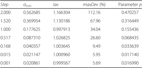
The proposed algorithm was encoded in the C program-ming language. The program outputs the best coefficients, the minimum achieved standard deviation, the average value of the intensities, and the maximum deviation of in-tensities from target values. The values of parameterpfor different search steps (step) (Table 4) are also contained in the program’s output. The results from Table 4 suggest that standard deviation of the maximum intensity devi-ation rapidly falls as the values of thestepdecrease.

A separate program written in C# used the text output of the main simulation and generated textual and graph-ical reports. Running of the actual program for different values ofn'showed that it produced the best results for

n'=_n. However, with increasing _n', the simulation time sharply increased and the simulation quickly became in-feasible. With the computer currently at our disposal (PC, CPU 3 GHz, 4GB RAM), the limit for simulations of reasonable length was set atn'= 13.

Figure 6 illustrates typical simulation results for the

“flat” target spectrum. It also indicates the position of the maximum of intensity deviation with respect to the intensity of the targeted spectrum. This particular ex-ample of spectrum synthesis serves a dual purpose: (i) the simplicity of the spectrum shape allows for easy ana-lysis of the errors introduced by the algorithm and (ii) a physical device with a flat output spectrum can serve as a very useful tool for calibration and characterization measurements of various types of spectrophotometers.

Table 2Number of iteration cycles forres= 0.005 and function (9)

Iteration numberc Function:1

2ðuba−lbaÞβ c

40 0.014781

41 0.013303

42 0.011973

43 0.010775

44 0.009698

45 0.008728

46 0.007855

47 0.007070

48 0.006363

49 0.005726

50 0.005154

Table 3Number of iteration cycles forres= 0.005 and function (10)

Iteration numberc Function:1

2ðuba−lbaÞβcln cðþ1Þ

15 0.012503

16 0.008428

17 0.005645

18 0.003757

Table 4Representative values of minimum standard deviation

σmin(7) and parameterp(16) as a function ofstepfor spectral range 700 - 1070 nm,lba= 0,uba= 4,n'= 13,β= 0.99

Step σmin Iav maxDev(%) Parameterp

2.000 0.562685 1.166304 112.16 0.470257

1.520 0.369954 1.130186 67.96 0.316449

1.000 0.177625 0.997913 34.04 0.155436

0.517 0.087310 1.026825 26.60 0.068435

0.168 0.040357 1.003645 9.49 0.033639

0.015 0.021147 1.000960 5.95 0.017140

Figure 7 illustrates the typical convergence pattern of a single LED coefficient (L850 in this example), as a func-tion of the iterafunc-tion numberc. Convergence of coefficients of the remaining LEDs in the array follows a similar pat-tern. It is readily apparent that the coefficient oscillates around the optimal value, with the amplitude of oscillations diminishing asc rises, according to the given logarithmic function (11). The iteration process is repeated until the amplitude of oscillations falls below the sought resolution.

Finally, Fig. 8 is a graphical representation of devia-tions from the targeted flat curve in the spectral range 700 - 1070 nm of the obtained spectrum. Due to the SPD characteristics of the LEDs used in the simulation (Figs. 1 and 2), deviations were mostly pronounced in the 840 - 860 nm spectral range (~5 %). In the rest of the spectrum they did not exceed 4 %.

Verification of the algorithm using programming package mathematica

The algorithmic solution presented in this paper was also verified with the computer algebra system MATHE-MATICA, which is highly applicable to problems that involve symbolic computations. Here, similar to what we did in our algorithmic solution, we adopted that the desired intensities I1, I2, …, Im have the same constant

value, i.e.I1=I2=…=Im= 1. Also, we addedεi,i¼1; m,

to the right sides of the equations from (1), whereεiis the

difference between the i-th obtained intensity Ii and the

desired light-emitting intensity valueIequal to 1 (17, 18). We also considered the limits (19) for the unknowns aj, j¼1;n:

X_n

j¼1ajMij¼1þεi; i¼1;m; ð17Þ

−1≤ε_i≤1; i¼1;m; ð18Þ

0≤_aj≤4; _j¼1;_n ð19Þ

The standard deviation of the dispersion of intensities (2) obtained in this way, compared to the desired intensity values equal to 1, needed to be minimized (21):

σ¼

ffiffiffiffiffiffiffiffiffiffiffiffiffiffiffiffiffiffiffiffiffiffiffiffiffiffiffiffiffiffiffi 1

m

Xm

i¼0ðIi−1Þ 2 r

¼

ffiffiffiffiffiffiffiffiffiffiffiffiffiffiffiffiffiffiffiffiffiffiffi 1

m

Xm

i¼0εi 2 r

ð20Þ

Therefore, we obtained the following single-objective optimization problem in (2), which was subjected to (17, 18, and 19).

min

ffiffiffiffiffiffiffiffiffiffiffiffiffiffiffiffiffiffiffiffiffiffiffi 1

m

X_m

i¼0εi 2 r

ð21Þ

The above-mentioned optimization problem is a vari-ation of the standard linear programming problem; it con-tains n+m unknowns and is subject to the constraints

Fig. 6_“Synthetized_”spectrum (solid line) and position of maximum deviation (maxDev) from flat spectrum (dashed line) in 700-1070 nm spectral range

Fig. 7Convergence pattern of simulation results (LED with peak at 850 nm) for the simulation presented in Fig. 6

determined bymequations andn+minequalities. There are several methods that can be applied to solve this prob-lem (e.g. see Tikhonov’s method [25–28]). The classical approach is to introduce so-called free variables, in order to transform the primal problem to its standard form, containing only equations. After that, the Simplex method is certainly the approach of choice for solving the obtained linear programming problem [29, 30].

A built-in MATHEMATICA function NMinimize[{f ,-cons},vars] minimizes the objective function f numeric-ally, subject to the constraints provided by the listcons, and variables given by the list vars. Therefore, the following implementation was considered:

MinDeviation½M List :¼Module½fm; n; cons; f; varsg;

m; n

f g ¼Dimensions½ M;

cons¼Union

"

Table X24

j¼1M½½ i;j a j½ ¼¼1þeps½ i;fi;1; mg

h i

;

Table½−1≤eps½ i ≤1;fi;1;mg;

Table 0½ ≤a j½ ≤4; fj;1;ng

#

;

vars¼Union Table eps½ ½ ½ i;fi;1;mg;Table½a j½ ;fj; 1; ng;

f¼Sqrt 1

mX_i¼1mðeps½ iˆ2Þ

" #

;

Return NMinimize f½ ½f ; consg; vars;;

The matrix M, where M= (Mij), 1≤i≤m, 1≤j≤n, is an SPD matrix of the LEDs extracted from Table 1. The dimensions of the matrix are m×n, where m is the selected spectral bandwidth and n is the number of selected diodes. For this matrix, the minimal standard deviation was equal to 0.019792.

Therefore, the maximal absolute declination was obtained for the coefficient ε37= 0.0565 = 5.65 %. Notice

that the constraints–1≤εi≤1,i¼1;min our

mathemat-ical model can be formulated as–0.06≤εi≤0.06,i¼1;m,

since the maximal absolute declination never exceeded 6 % in our computations in MATHEMATICA.

The solutions obtained by means of this software showed considerable overlaps with the data received from our method (Table 5).

Comparison with an existing algorithmic solution

In order to evaluate potential merits of the newly-developed algorithm, a comparison was made with the algorithmic solution described in [15]. This previously-published algorithm solely depends on the minimization of parameterp(16). To make a meaningful comparison, the same set of assumptions were made as in [15]: individual LED spectra were taken as having a Gaussian

Table 5LED coefficients obtained with MATHEMATICA software and our algorithmic solution for a“flat”curve in the spectral range 700 - 1070 nm

Spectral range 700 - 1070 nm

LED Coefficient Mathematica Our algorithm

L680 a1 0.758 0.825

L690 a2 0.020 0.002

L700 a3 0.558 0.559

L710 a4 0.260 0.261

L720 a5 0.411 0.410

L735 a6 0.560 0.560

L750 a7 0.346 0.346

L760 a8 0.328 0.327

L770 a9 0.185 0.186

L780 a10 0.480 0.479

L800 a11 0.478 0.479

L810 a12 0.401 0.401

L820 a13 0 0

L830 a14 0.354 0.354

L850 a15 0.633 0.633

L870 a16 0.240 0.240

L890 a17 0.606 0.607

L910 a18 0.280 0.279

L940 a19 0.731 0.731

L970 a20 0.012 0.012

L980 a21 0.570 0.569

L1020 a22 0.482 0.482

L1050 a23 0.324 0.325

L1070 a24 0.815 0.815

σ(standard deviation) 0.020860 0.020861

Maximum deviation (%) 5.68 5.69

shape with 20 nm FWHM. The simulations were per-formed for the visible spectrum (380 - 780 nm). The peek wavelengths for a given set of LEDs were chosen to be equidistant at 20, 10 and 5 nm. This effectively means that three sets of 20, 40 and 80 LEDs, respectively, were tested. The validity of our optimization algorithm was tested for two well-known light spectra: CIE standard daylight illuminant D65 and HMI HID lamp. The simulation results with 5 nm LED intervals for the spectral range 380 – 780 nm are presented in Figs. 9 and 10. The figures show that the proposed algorithm simulated the spectra very accurately.

Table 6 shows a comparison between the results for parameter p of the two different algorithms. It is im-mediately apparent that the new algorithm yielded some-what better results (lower value of p) for the 20 nm distance between peeks. For more densely populated sets of LEDs (10 nm and 5 nm inter-peak distance), our algorithm produced the same or slightly higher values ofp

for the CIE D65 and HMI HID lamps.

Based on the presented comparisons, we believe that the newly-developed algorithm offers some improve-ments, particularly in the case of sparsely populated sets of LEDs and/or target SPDs with more pronounced peeks.

Simulation of blackbody radiation

One of the SPDs of particular interest in our research was the spectrum of blackbody radiation in VNIR (700

-1070 nm,) corresponding to blackbody temperatures above 800 °C [31, 32]. As previously mentioned, this kind of source could be useful for the calibration of optical pyrometers that operate in the range from 700 to 1070 nm.

Synthesis of Planck’s curve in the given wavelength interval and for the temperatures of interest presented an additional challenge for the algorithm described in this paper. Namely, the spectra cover a very broad dy-namic range with orders-of-magnitude different inten-sities at the endpoints. Our algorithm is limited in the sense that uba determines the dynamic range of the

synthetized spectrum. To address this problem, the ini-tial values of the lower (lba) and upper (uba) boundaries

for the coefficientsajwere changed. Thus, fort =800 °C

boundaries they were lba= 0 and uba= 4, while for t=

1300 °Cubawas increased touba= 30. It was also

deter-mined that for this kind of target SPD, the optimal value of parameterβwasβ= 0.992.

Using the modifications mentioned in the previous para-graph, the newly-developed algorithm was applied to a set of real LEDs (using real SPDs for each LED from the set), in order to derive the intensity coefficientsajand simulate

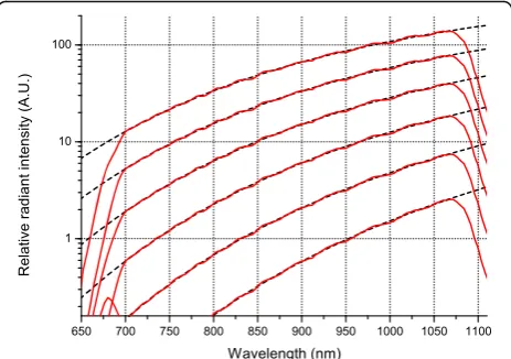
Planck’s law curve for temperatures between 800 °C and 1300 °C. Representative results of these simulations are pre-sented in Fig. 11. Numerical results of the simulations for three different temperatures are given in Table 7, along with the values of aj calculated using MATHEMATICA

software. The similarity of the coefficients obtained by our algorithm and MATHEMATICA was yet another verifica-tion of the validity of our approach.

In order to verify that the synthesized blackbody spectra can indeed be used for calibrating optical pyrometers, the errors introduced by this non-ideal calibration source needed to be estimated. The basic assumption was that in the 800 - 1300 °C temperature range, the most common sensors used in pyrometry are PIN diodes with typical spectral sensitivity characteristics in the spectral range 600 - 1100 nm, as illustrated in Fig. 12 [33–35].

The output voltage of the PIN diode amplifier is propor-tional to the spectral radiance and for the spectral range (λ1,λ2) it depends on the blackbody temperature as:

Uð Þ ¼T C

Z λ2

λ1

Nðλ;TÞSð Þλ dλ ð22Þ

Fig. 10SPD of an HMI HID lamp (solid line) and our simulation results with 5 nm LED intervals (circles)

Table 6Parameter_pfor wavelength intervals over the spectral range from 380 nm to 780 nm

Algorithm with functionβcln(c+ 1) _{I. Fryc, S. W. Brown and Y. Ohno algorithm [15]}

LED’s peak wavelength intervals 20 nm 10 nm 5 nm 20 nm 10 nm 5 nm

Parameterpfor target light source CIE D65 0.040 0.004 0.004 0.079 0.004 0.003

HMI HID 0.042 0.011 0.010 0.074 0.008 0.007

where: C is the proportionality constant which includes amplification and optical characteristics of a sensor and optical parts of the pyrometer, and S(λ) is the spectral responsivity of the PIN diode. The quantity Nλ(λ,T) is the spectral radiance in the given temperature range and can be derived from Planck’s law:

Nλðλ;TÞ ¼2hc

2

λ5 1

eλkBThc −1 ð23Þ

By substituting the values of the ideal blackbody spec-tral radiance (23) with radiance values obtained from the simulation, it is possible to calculate the difference in temperature readings between the ideal blackbody and the synthesized calibration source.

Our calculations showed that the errors in tem-perature readout due to the non-ideality of the LED

Fig. 11Blackbody relative radiant intensities for 800, 900, 1000, 1100, 1200 and 1300 °C (dashed lines) and LED SPDs (solid lines) for the spectral width of 700 - 1070 nm

Table 7LED coefficients produced by MATHEMATICA and our algorithmic solutions for different temperatures in the spectral range 700 - 1070 nm

SPD of LEDs for Planck’s law in the spectral range 700 - 1070 nm

LED Coefficient Temperature 800 °C Temperature 1000 °C Temperature 1200 °C

Mathematica Our algorithm Mathematica Our algorithm Mathematica Our algorithm

L680 a1 0.008 0.023 0.290 0.215 2.893 3.770

L690 a2 0.004 0 0 0.012 0 0

L700 a3 0.013 0.013 0.319 0.325 2.893 2.727

L710 a4 0.010 0.010 0.171 0.168 1.497 1.570

L720 a5 0.014 0.015 0.295 0.297 2.565 2.532

L735 a6 0.031 0.030 0.542 0.542 4.407 4.417

L750 a7 0.020 0.021 0.362 0.362 2.916 2.906

L760 a8 0.030 0.029 0.478 0.479 3.593 3.592

L770 a9 0.015 0.015 0.233 0.231 1.792 1.786

L780 a10 0.054 0.054 0.834 0.835 6.048 6.051

L800 a11 0.067 0.065 0.955 0.955 6.701 6.700

L810 a12 0.074 0.074 1.008 1.008 6.753 6.754

L820 a13 0 0 0 0 0 0

L830 a14 0.076 0.076 1.003 1.002 6.548 6.547

L850 a15 0.190 0.190 2.298 2.298 14.156 14.156

L870 a16 0.072 0.072 0.930 0.930 5.803 5.804

L890 a17 0.322 0.323 3.401 3.401 19.004 19.004

L910 a18 0.156 0.156 1.681 1.682 9.371 9.371

L940 a19 0.662 0.663 6.226 6.226 31.796 31.796

L970 a20 0 0 0 0 0.029 0.029

L980 a21 0.706 0.706 6.188 6.188 29.972 29.972

L1020 a22 0.802 0.801 6.499 6.498 29.740 29.740

L1050 a23 0.571 0.571 4.617 4.617 20.981 20.981

L1070 a24 2.273 2.273 16.032 16.032 66.493 66.492

σ(standard deviation) 0.022123 0.022124 0.181485 0.181485 0.855000 0.855004

source did not exceed 0.1 °C in the temperature range of interest.

Conclusion

This paper examined the feasibility of using a set of LED sources whose cumulative output simulated the “flat” spectrum as well as the blackbody radiation spectrum in the 700 - 1070 nm interval and in the 800 - 1300 °C temperature range. Our research team intends to use the actual composite LED source primarily to calibrate op-tical pyrometers. We developed a novel algorithm that calculates the intensities of each individual LED in the composite source, in order to achieve the desired output spectral profile. Apart from the “flat” and blackbody spectra, the algorithm was tested on various other target spectral profiles. Especially the “flat” spectrum which is very important as it might enable evaluation and direct measurements of spectral responses of various types of optical sensors and systems. We demonstrated that the proposed algorithm compares favorably with other methods for shaping the output spectral profile of tunable LED light sources. It provides an efficient theoretical base for practical realization of calibration sources.

Abbreviations

CIE:International Commission on Illumination; FWHM: Full width at half maximum; HID: High intensity discharge; HMI: Hydrargyrum medium-arc iodide; LED: Light emitting diode; SPD: Spectral power distribution; VNIR: Very near infrared region

Acknowledgment

The light spectra data of the CIE standard daylight illuminant D65 and HMI HID lamp were obtained from the National Institute of Standards and Technology (NIST), courtesy of Irena Fryc, private communication–Bialystok University of Technology, Poland.

Funding

This ongoing research is funded was funded by the Ministry of Education, Science and Technological Development under project No. 171035.

Authors’contributions

ML developed the proposed algorithm for tunable light sources and carried out all the simulations. VL programmed the algorithm in C and the graphical view of the algorithm in C#. IB proposed the specification and the initial design of the tunable light source. BK provided expert advice. IS programmed the algorithm using Mathematica software. MV coordinated the work and contributed to writing. All the authors have read and approved the final manuscript.

Competing interests

The authors declare that they have no competing interests.

Author details

1_{University of Kragujevac, Faculty of Technical Sciences, Cacak 32000, Serbia.} 2

University of Belgrade, Faculty of Physics, Belgrade 11000, Serbia.3University of Nis, Faculty of Science and Mathematics, Nis 18000, Serbia.

Received: 13 August 2016 Accepted: 18 October 2016

References

1. Ries, H., Leike, I., Muschaweck, J.: Optimized additive mixing of colored light-emitting diode sources. Opt. Eng.43, 1531–1536 (2004)

2. Li, Y.-L., Shah, J.M., Leung, P.-H., Gessmann, T., Schubert, E.F.: Performance characteristics of white light sources consisting of multiple light emitting diodes. Proc. SPIE5187, 178_–184 (2004)

3. Shang, P. Y., Tang, C. W., Huang, B. J.: Charaterizing LEDs for mixture of colored LED light sources, in 2006 Int. Conf. Electron. Mater. Packag. EMAP 2006, (IEEE, Kowloon, 2006)

4. Lu, S.S.L.W., Zhang, T., He, S.M., Zhang, B., Li, N.: Light-emitting diodes for space applications. Opt. Quant. Electron.41, 883–893 (2009)

5. Finlayson, G., Mackiewicz, M., Hurlbert, A., Pearce, B., Crichton, S.: On calculating metamer sets for spectrally tunable LED illuminators. J. Opt. Soc. Am. A Opt. Image Sci. Vis.31, 1577_–1587 (2014)

6. Hirvonen, J.M., Poikonen, T., Vaskuri, A., Kärhä, P., Ikonen, E.: Spectrally adjustable quasi-monochromatic radiance source based on LEDs and its application for measuring spectral responsivity of a luminance meter. Meas. Sci. Technol.24, 115201_–115208 (2013)

7. Mackiewicz, M., Crichton, S., Newsome, S., Gazerro, R., Finlayson, G. D., Hurlbert, A.: Spectrally tunable led illuminator for vision research, in Conf. Colour Graph. Imaging, Vision, CGIV 2012, (Society for Imaging Science and Technology, Amsterdam, 2012)

8. Kolberg, D., Schubert, F., Lontke, N., Zwigart, A., Spinner, D.M.: Development of tunable close match LED solar simulator with extended spectral range to UV and IR. Energy Procedia8, 100–105 (2011)

9. Kasalica, B.V., Belca, I.D., Stojadinovic, S.D.J., Zekovic, L.J.D., Nikolic, D.: Light-emitting-diode-based light source for calibration of an intensified charge-coupled device detection system intended for galvanoluminescence measurements. Appl. Spectrosc.60, 1090–1094 (2006)

10. O_’Hagan, W.J., McKenna, M., Sherrington, D.C., Rolinski, O.J., Birch, D.J.S.: MHz LED source for nanosecond fluorescence sensing. Meas. Sci. Technol. 13, 84–91 (2002)

11. Fryc, I., Brown, S.W., Ohno, Y.: A spectrally tunable LED sphere source enables accurate calibration of tristimulus colorimeters. Proc. SPIE 6158, 61580E (2004)

12. Brown, S.W., Santana, C., Eppeldauer, G.P.: Development of a tunable LED-based colorimetric source. J. Res. Natl. Inst. Stand. Technol. 107, 363_–371 (2002)

13. Fryc, I., Brown, S.W., Eppeldauer, G.P., Ohno, Y.: LED-based spectrally tunable source for radiometric, photometric, and colorimetric applications. Opt. Eng. 44, 111308–111309 (2005)

14. Burgos, F. J., Perales, E., Herrera-Ramírez, J. A., Vilaseca, M., Martínez-Verdú, F. M., Pujol, J.: Reconstruction of CIE standard illuminants with an LED-based spectrally tuneable light source, in 12th Int. AIC Congr. AIC2013, (2013) 15. Fryc, I., Brown, S.W., Ohno, Y.: Spectral matching with an LED-based

spectrally tunable light source. Proc. SPIE5941(59411I), 300_–308 (2005) 16. Brown, S.W., Rice, J.P., Neira, J.E., Johnson, B.C., Jackson, J.D.: Spectrally

tunable sources for advanced radiometric applications. J. Res. Natl. Inst. Stand. Technol.111, 401–410 (2006)

17. Yuan, S.J., Huimin Yan, K.: LED-based spectrally tunable light source with optimized fitting. Chinese Opt. Lett.12, 32301 (2014)

18. Hsu, C.-W., Hsu, K.-F., Hwang, J.-M.: Stepless tunable four-chip LED lighting control on a black body radiation curve using the generalized reduced gradient method. Opt. Quant. Electron.48, 1–8 (2016)

19. Lasertechnik, R.: Roithner Lasertechnik - LEDs. 2014, <http://www.roithner-laser.com/led.html> Accessed 9 Apr 2014

20. Van Benthem, M.H., Keenan, M.R.: Fast algorithm for the solution of large-scale non-negativity-constrained least squares problems. J. Chemom. 18, 441–450 (2004)

21. Chalmers, A., Soltic, S.: Light source optimization: spectral design and simulation of four-band white-light sources. Opt. Eng.51, 044003_–1 (2012) 22. Kim, H., Park, H., Eldén, L.: Non-negative tensor factorization based on

alternating large-scale non-negativity-constrained least squares, in Proc. 7th IEEE Int. Conf. Bioinforma. Bioeng. (BIBE, Boston, 2007)

23. Bro, R., Jong, S.: A fast non-negativity-constrained least squares algorithm. J. Chemom.11, 393–401 (1997)

24. Rokhlin, V., Tygert, M.: A fast randomized algorithm for overdetermined linear least-squares regression. Proc. Natl. Acad. Sci.105, 13212–13217 (2008)

25. Lampe, J., Voss, H.: Large-scale Tikhonov regularization of total least squares. J. Comput. Appl. Math.238, 95–108 (2013)

26. Golub, G.H., Hansen, P.C., O’Leary, D.P.: Tikhonov regularization and total least squares. Siam J. Matrix Anal. Appl.21, 185_–194 (1999)

27. Wei, Y., Zhang, N., Ng, M.K., Xu, W.: Tikhonov regularization for weighted total least squares problems. Appl. Math. Lett.20, 82–87 (2007) 28. Beck, A., Ben-Tal, A.: On the solution of the Tikhonov regularization of the

total least squares problem. SIAM J. Optim.17, 98_–118 (2006) 29. Nash, J.C.: The (Dantzig) simplex method for linear programming.

Comput. Sci. Eng.2, 29–31 (2000)

30. Forrest, J.J., Goldfarb, D.: Steepest-edge simplex algorithms for linear programming. Math. Program.57, 341_–374 (1992)

31. Planck, M.: The theory of heat radiation. Search30, 85–94 (1914) 32. Chandrasekhar, S.: Radiative Transfer, in Energy (Dover Publication Inc, New

York, 1960)

33. Photonics H.: Characteristics and use of infrared detectors, Small, 43 (2004) 34. Bellotti, E., D’Orsogna, D.: Numerical analysis of HgCdTe simultaneous

two-color photovoltaic infrared detectors. IEEE J. Quantum Electron. 42, 418–426 (2006)

35. Rogalski, A.: Infrared detectors: an overview. Infrared Phys. Technol. 43, 187–210 (2002)

36. OSI Optoelectronics: Two Color Sandwich Detectors. Silicon Photodiodes, 2015, <http://www.osioptoelectronics.com/standard-products/silicon-photodiodes/two-color-sandwich-detectors.aspx> Accessed 2 Apr 2016.

Submit your manuscript to a

journal and benefi t from:

7Convenient online submission

7Rigorous peer review

7Immediate publication on acceptance

7Open access: articles freely available online 7High visibility within the fi eld

7Retaining the copyright to your article