Model modulation to add smaller scale structures to large scale electron density models

(1)

SRef-ID: 1684-9973/ars/2005-3-441

Advances in

Radio Science

Model modulation to add smaller scale structures to large scale

electron density models

R. Leitinger, E. Feichter, and M. Rieger

Institut f¨ur Geophysik, Astrophysik und Meteorologie, Universit¨at Graz, Austria

Abstract. Usually regional and global electron density mod-els provide large scale spatial structures only and smooth out the smaller scale features of the electron density distribution. We present a method to modulate existing electron density models by multiplication:M(h, ϕ, λ, t )=L(h, ϕ, λ, t )× S1(h, ϕ, λ, t )×S2(h, ϕ, λ, t )× · · ·Sn(h, ϕ, λ, t )

M: resulting electron density distribution, L: large scale model,S1· · ·Sn: modulating models for n the smaller scale structures;h: height;ϕ, λ: geographic coordinates,t: Uni-versal Time. There are no restrictions to the nature of the large scale model provided it takes height and horizontal co-ordinates as input. Examples are models of the “profiler” type which use large scale “maps” for profile anchor points (e.g., E, F1, F2 peak properties) like the International Ref-erence Ionosphere (IRI). Typical examples for smaller scale structures are ridges, troughs and wavelike disturbances. The advantage of modulation by multiplication is that there is no danger to get zero or negative values of electron density as long as the background and modulations are>0 everywhere. For each modulation model, unity means “undisturbed”.

1 Introduction

Large scale electron density models of the “profiler” type like the International Reference Ionosphere (IRI)(Bilitza, 2001) or the “model family” developed at Graz and Trieste use an-chor points to which the height profile of electron density is attached. These anchor points are the peaks of the iono-spheric “layers” E, F1 und F2. For monthly median condi-tions the models use “maps” from which the anchor point properties are derived. The “maps” are algorithms which al-low to calculate the critical frequencies foE, foF1, foF2 and the F2 layer transfer parameter M3000(F2).

The profiler models mentioned allow updating with mea-sured values, a procedure adequate only for single height

Correspondence to: R. Leitinger

([email protected])

profiles of electron density. Updating of slant profiles, e.g., along straight lines between arbitrarily chosen end points, could be done on a regional basis with special maps con-structed by means of “instantaneous mapping procedures”. For the model family NeQuick, COSTprof and NeUoG– plas (Leitinger et al., 2000) a “data grid” method was pro-posed, successfully implemented and used (Leitinger et al., 2001, 2002). The global grids have a spacing of 2.5◦in lati-tude and 5.0◦in longitude. A cyclic third order interpolation scheme is used to gain values between the grid points. The latitude and longitude resolution of the data grids is compa-rable to that of the ITU–R (formerly CCIR) maps.

The map or data grid resolution is sufficient for large scale ionospheric structures only. Necessarily the temporal reso-lution is coarse too: the ITU–R maps exist for each month and each hour UT only. Data grids could be constructed for denser temporal spacing but it is not realistic to plan for time intervals smaller than 15 min.

Our modulation method allows to superimpose smaller scale and time dependent structures.

2 The modulation method

Assuming that the large scale model is given as

L=L(h, ϕ, λ, t )and that we have several different modula-tions (S1, S2, · · · Sn) we gain the resulting electron density distributionMas

M(h, ϕ, λ, t )=L(h, ϕ, λ, t )×S1(h, ϕ, λ, t )×

S2(h, ϕ, λ, t )× · · ·Sn(h, ϕ, λ, t )

h: height;ϕ, λ: geographic coordinates,t: Universal Time.

S1 · · · Sn must be positive definite functions (being ev-erywhere and at all times>0), unity (Sk =1) meaning “no disturbance”, 0< Sk<1 meaning “electron density depres-sion”,Sk >1 meaning “electron density enhancement”.

(2)

0 1 2 3 4 5 -2

-1 0 1 2

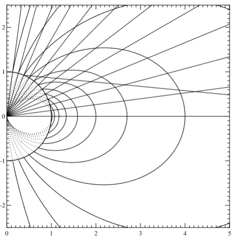
Fig. 1. Relation between ray path, magnetic and geocentric

coordi-nates demonstrated by means of centric dipole coordicoordi-nates. Straight line rays in a meridian plane. Shells of constant magnetic latitude give dipole field lines in the meridian plane; the surfaces of constant geographic latitudes are concentric cones. There are three possibili-ties for the relation of the ray to a specific magnetic shell: (a) it cuts the shell twice; (b) it is tangent to the shell; (c) it has no intersection at all if the magnetic latitude is too low. In case (a) the lower inter-section point has a larger geocentric latitude than the upper one. The model trough minimum is represented by the magnetic shell which represents its magnetic latitude. Note that invariant mag-netic coordinates are calculated with three dimensional field lines and therefore the geometric situation is a bit more complicated.

the model is larger than a few minutes, Fourier or spline in-terpolation is an adequate method. Gliding third order inter-polation might be adequate too and has the advantage that 4 sets of data grids are sufficient at any model time.

3 The model for the main trough of the F layer

A complete three dimensional formulation for the main trough has been constructed on the basis of Dynamic Ex-plorer (DE) data (Leitinger and Feichter, 1999)(Feichter and Leitinger, 2002). The model uses the trough minimum model published by Werner and Pr¨olss (1995) (which is also based on DE data) and a time dependent shape of the trough. The shape parameters

– depth of the trough, – equatorward half–width, – poleward half–width,

– steepness of the equatorward wall, – steepness of the poleward wall

have been derived from Dynamic Explorer electron densities gained in the height region below 700 km and scaled to the

0.0 0.2 0.4 0.6 0.8 1.0 1.2

east -0.6

-0.4 -0.2 -0.0 0.2

north

Fig. 2. TID fan beam, projected onto the surface of the earth. Horizontal half width: 30◦, azimuth of center: 120◦,

F2 layer peak by means of the COSTprof model. Our trough model uses the medians of the shape parameters for three seasons (winter, equinox, summer) and two magnetic local time intervals (“day” and “night”)(see Feichter and Leitinger (2002) for statistics). After several tests we settled on a com-posite for the trough shape. The trough consists of two parts, an equatorward one and a poleward one. Both parts use el-lipse sectors for bottom and top joined together by straight lines in such a way that the first derivatives are continuous. The equatorward and poleward parts meet at the trough min-imum. Added to the poleward part is a 20% enhancement which fades out like a Gaussian. For examples of the trough shape see Feichter and Leitinger (2002).

In accordance with the “modulation” requirements the trough model uses height and geographic coordinates as ex-plicit input but depends on

– geomagnetic activity, – season

– Universal Time.

Internally the trough model depends on magnetic coordi-nates which are calculated from the geographic coordicoordi-nates, height, date and time. Since the model for the position of the trough minimum published by Werner and Pr¨olss (1995) uses Invariant Coordinates we have adopted the same type of magnetic coordinates. Magnetic coordinates ensure that the trough features like the walls of the trough are geomagnetic field aligned.

Since magnetic latitude is constant for a given magnetic “shell” all trough features are automatically magnetic field aligned.

4 The TID model

(3)

0 100 200 300 longitude (deg. E)

40 50 60 70 80 90

latitude (deg. N)

16.7

25

25 ₂₅

25

33.3

33.3 33.3

33.3

50

50 50 50

100

Fig. 3. Example for trough modulation: electron density of the

ITU-R (CCIITU-R) “map” for October, 0 UT,R12=100 modulated with the main trough forKp = 6. Isolines of electron density in units of 1010m−3in a geographic coordinate system.

4.1 Atmospheric Gravity Waves (AGWs)

Since we are not dealing with the propagation of AGWs through a realistic atmosphere but need their basic proper-ties only, we can assume validity of the dispersion relation of AGWs in its simplest form (Hines, 1960)

k2_z =ω 2 b−ω2

w2 k

2 x−

ω_a2−ω2 c2

s

ωbis the (isothermal) Brunt-Väisälä frequency,ωathe acous-tic cut-off frequency,ωthe (angular) frequency of the AGW,

kxthe horizontal,kzthe vertical wave number,cs is the ve-locity of sound.

ω2_b= (γ −1)g 2

c2 s

, ωa=

γ g

2cs

Defining horizontal and vertical refractive indices nx =

kxcs/ω and nz =kzcs/ω and

a2=

1−ω 2 a

ω2

1−ω 2 b

ω2

, b2=1−ω

2 a

ω2,

gives after re–arrangements n 2 x

a2 +

n2_z

b2 =1.

This is the equation for a conic section with axesa2andb2,

a2= α b

2

α−(1−b2₎ with α=ω

2 a

ω2_b

= γ

2

4(γ −1)>1.

(γ =1,4→α=1,225). The velocity of sound is given by

c_s2=γ H g (H: pressure scale height of the atmosphere,g: acceleration of gravity).

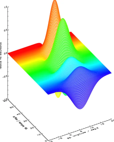
Fig. 4. TID modulation at 250 km, 3-D display. Wave period 60 min, hor. wave length 200 km, source point 70◦N, 15◦E, fan half width 5◦, azimuth 195◦.

Real solutions exist in two cases:

1. b2>0 (and also a2 >0), meaningω2> ω_a2. This is the “acoustic branch”, the index surfaces are ellipsoids. The refraction indices are always<1. For ω → ∞

the surfaces degenerate into spheres what corresponds to the propagation of “normal” sound with the phase velocity cs . No dispersion and no anisotropy.

2. b2 < 0 and a2 > 0, meaning ω2 < ω_b2. This is the branch of “gravity waves” (“buoyancy waves”), the index surfaces are hyperboloids. The refractive indices are always> 1. For ω → 0 the index surfaces de-generate into circular cylinders: a2 → ∞, b2 → −0,225 (for γ =1,4).

Withc2= −b2we have the hyperboloid equation

n2_x a2 −

n2_z

c2 =1, −→ n

2 z=c

2 n2x

a2 −1 !

.

A (gravity branch) AGW can be defined by ω < ωb (or

τ > τb) and kz. kz and ω give nx, a, c and finally nz,

(4)

Fig. 5. TID modulation at 250 km, contour line display. TID properties as for Fig. 4. Red: positive values, blue: negative values.

4.2 TIDs as plasma signatures of AGWs

To find the plasma signature of an AGW we need the equa-tion of continuity for the electron density

∂Ne

∂t =q−L−∇·(Neue)

Ne: electron density; ue: electron velocity. Perturbation ansatz (compare, e.g., Leitinger (1992)): Ne = Neo +

Ne1, ue =ueo+ue1. Indexo: background, index 1: per-turbation (induced by AGW).

Neglecting a background electron “wind” (settingue0 = 0) and assuming that the passing AGW influences the elec-trons only by the transport term (no effect on production and loss) gives

∂Ne

∂t = −∇·(Neoue1)

The relation ofu_e1tounis given by a balance between the Lorentz force and the “ion drag” force:

e (ue1 × B)+meνen(ue1−un)=0

(B: geomagnetic induction vector;e: electron charge; me: electron mass;νen: effective collision frequency).

Introducing the unit vector of the geomagnetic fieldbby

B =Bband the electron gyro frequency ωg = (e / me) B gives the solution

ue1=

1+α2

−1

α2un−αun×b+(un·b)b

with α=νen ωg

In the F region νen<< ωg which justifies the approximation

ue1=. (un·b)b.

A monochromatic wave in un gives a monochromatic wave inue1 and inNe1. Using a relevant ansatz allows to replace∂A / ∂tbyj ω Aand∇AbyjkA (j =

√ −1).

j ω Ne1=(un·b)[j (k·b) Ne0−(b·∇) Neo]

Ne1=

(un·b)

ω [(k·b)−j (b·∇)]Neo

If the second term in[ ]can be neglected we approximate

Ne1

Neo

.

=k (un·b)

ω cos(4)

Since we have a real and an imaginary part ofun =ur+jui

(un·b)=(ur·b)+j (ui·b)

Using local Cartesian coordinates(x, y, z)

k=



 kx

ky

kz



, ur =



 urx

ury

urz



, ui=



 uix

uiy

uiz



, b=



 bx

by

bz





gives cos(4)=kxbx+kyby+kzbz,

(un·b)=(urxbx+uryby+uzbrz)+

j (urxbx+uryby+urzbz)= |(un·b)| exp(j 9)

Ne1

Neo

. =

(un·b)

vph

cos(4)cos[kxs+kzh+9(h)−ωt] The phase constant9 reflects the polarization of the AGW: According to Beer (1974), the ratio of horizontal to vertical AGW wind velocity components is

c_s2[kz+j / (2H )] −j g kx

ω2₋_c2 sk2x

leading to

tan8= γ −2

2γ kxH

.

Since we have assumed height constantγ , kx, Hthe phase constant of the AGW,8, but not that of the TID,9, is inde-pendent of height.

(5)

tau=60 min, hor.wavelength= 500 km, transmitter moves S to N with 3 deg. / min.

10 20 30 40 50 60 70

transmitter latitude (deg. N) -15

-10 -5 0 5 10 15

tau=60 min, hor.wavelength= 500 km, transmitter moves N to S with 3 deg. / min.

10 20 30 40 50 60 70

-10 -5 0 5 10 15

10 20 30 40 50 60 70

-4 -2 0 2 4 6

10 20 30 40 50 60 70

-4 -2 0 2 4 6

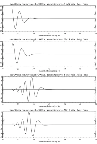
Fig. 6. TID modulation in slant electron content for a ground station at 45◦N, 15◦E and a (satellite) transmitter moving at 1000 km with 3 degrees per minute in the meridian plane of the ground station. TID properties: Source point at 70◦N, 30◦E, fan beam with half width of 10◦, azimuth of center: 190◦. With panel numbers 1 for top, 4 for bottom: wave periods 60 minutes (panels 1 and 2) and 30 min (panels 3 and 4); horizontal wavelengths 500 km (panels 1 and 2) and 300 km (panels 3 and 4); transmitter at a height of 1000 km moves S to N (panels 1 and 3) or N to S (panels 2 and 4).

with exp[(h−ho)/(2H )](needed to compensate for the ex-ponential decrease of neutral atmosphere density) and damp-ing through ion drag. Since there is indication that the rela-tive amplitude of LSTIDs peaks below the F layer peak we have chosen a Chapman layer type height dependence:

|Un|

vph =

_|_U

n|

vph

0 exp

1−z−exp(−z)

with z= h−ho HCh

ho being the height of the amplitude maximum, HCh a thickness parameter.

(6)

for-tau=60 min, hor.wavelength= 500 km, transmitter moves S to N with 3 deg. / min.

10 20 30 40 50 60 70

transmitter latitude (deg. N) 0

500 1000 1500 2000 2500

sTEC / 10

15 m

-2

10 20 30 40 50 60 70

500 1000 1500 2000 2500

sTEC / 10

15 m

-2

10 20 30 40 50 60 70

500 1000 1500 2000 2500

sTEC / 10

15 m

-2

10 20 30 40 50 60 70

500 1000 1500 2000 2500

sTEC / 10

15 m

-2

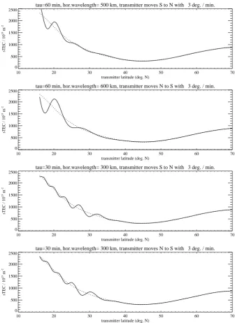
Fig. 7. NeQuick for October, 12:00 UT, solar activity parameter R12 = 150 modulated with the TID disturbances used for Fig. 6. Slant electron content in units of 1015m−2vs. geogr. latitude of the transmitter.

mulaA(σ )=A(σo)cosκ[(σ−σo)/2], σ being the azimuth of a ray emitted from the source point,σobeing the azimuth in which the maximum amplitude is emitted. Small beams need large values ofκ: A half width ofδ degrees needs ap-proximatelyκ =. 18 200/δ2(valid ifδ <10 degrees), e.g.,

δ=2 degrees needsκ =4550.

It is also appropriate to include geometric dilution of the TIDs. Distribution of wave energy over a sphere leads to a dilution of the amplitudes proportional to 1/

√

sin9. To avoid problems with the source point (9 = 0) we use 1/√1+(sin9 /sin9o)instead.

Finally, ion drag extracts energy from the AGW which means that we have to take attenuation into account. We

have chosen attenuation according to exp(−9/9∗) with

9∗=π λs/ Re.

The simplifying assumptions are sufficiently good for the “far field” in the F region but should not be applied in the vicinity of the source region of the AGWs and not in the E region.

4.3 (MS and LS) TID modulation The TID model adopted:

– The TIDs are assumed to be plasma signatures of At-mospheric Gravity Waves (AGWs)

(7)

– a TID travels in a “fan beam” defined by its azimuth and its half width

– the wave properties are given by the wave periodτ and by the horizontal wave lengthλh

– for the vertical structure a Chapman profile was adopted defined by a scale heightHT and by a peak heighthmT. Values chosen for the examples shown:HT =100 km,

hmT =250 km

– the forward tilt of the wave fronts is produced via a height dependent phase constant9 in accordance with the dispersion relation of the AGWs

– the geometric dilution of horizontally traveling AGWs and horizontal attenuation are also taken into account – the model allows superposition of several TID wave

trains.

The following properties of the AGW are needed. – Horizontal componentkx and vertical componentkzof

the wave vectork

– AGW periodτ =2π / ω

– Velocity of the disturbanceun =Uncos[kxs+kzh+

8(h)−ωt] (s: horizontal coordinate,h: height,t: time,

9is a height dependent phase constant. Derived quantities:

λx =2π / kx; λz =2π / kz: horizontal and vertical wave lengths;

λ = 2π / k: (total) wave length (k = |k| = q

k2 x+kz2);

ω / k =ω /

q k2

x+kz2 = vph: phase velocity (to be distin-guished fromvh=ω/ kxthe horizontal phase velocity.

5 Modulation examples

A few examples for model modulation are shown here: Fig. 3 shows an F2 layer peak density map modulated with the main trough. For more examples of trough modulations see Leitinger et al. (2002).

Figures 4 and 5 are two different displays of a large scale TID modulation in electron density at 250 km height (peak of the TID amplitude). An example for the TID modulation in electron content is shown in Fig. 6. Modulated electron content is displayed in Fig. 7.

6 Conclusions

The method to “modulate” electron density models by mul-tiplication is very versatile. Since the sub–models are time dependent, we are able to provide realistic “scenarios” for assessment and case studies. We can introduce highly dy-namic structures for which the wavelike TID disturbances are only one example. More dynamic structures are in con-struction, e.g., equatorial “bubbles”, high latitude “blobs” and “patches” and soliton like disturbances to imitate some of the observations made during ionospheric storms.

References

Beer, T.: Atmospheric waves, Wiley, New York and Toronto, 1974. Bilitza, D.: International Reference Ionosphere 2000, Radio Sci.,

36, 261–275, 2001.

Feichter, E. and Leitinger, R.: Properties of the main trough of the F region derived from Dynamic Explorer 2 data, Ann. Geophysics, 45, 117–124, 2002.

Hines, C. O.: Internal atmospheric gravity waves at ionospheric heights, Canad. J. Phys., 38, 1441–1481, 1960.

Leitinger, R.: Travelling Ionospheric Disturbances (TIDs): Wis-sensstand und neuere Entwicklungen, Kleinheubacher Ber., 35, 1–14, 1992.

Leitinger, R. and Feichter, E.: Modelle f¨ur den Trog der F Schicht: M¨oglichkeiten und Grenzen, Kleinheubacher Ber., 42, 63–70, 1999.

Leitinger, R., Hochegger, G., Hafner, J., Radicella, S., and Nava, B.: NeQuick, COSTprof, NeUoG-plas – eine Familie von Ionosph¨arenmodellen, Kleinheubacher Ber., 43, 20–25, 2000. Leitinger, R., Nava, B., Hochegger, G., and Radicella, S.:

Iono-spheric profilers using data grids, Phys. Chem. Earth(C), 26, 293–301, 2001.

Leitinger, R., Radicella, S., and Nava, B.: Electron density models for assessment studies – new developments, Acta Geodet. Geo-phys. Hung., 37, 183–193, 2002.