Implementation and clinical application of a deformation method for fast simulation of biological tissue formed by fibers and fluid

M E T H O D O L O G Y

Open Access

Implementation and clinical application of

a deformation method for fast simulation

of biological tissue formed by fibers and

fluid

Ana Gabriella de Oliveira Sardinha

, Ceres Nunes de Resende Oyama

, Armando de Mendonça Maroja

and

Ivan F. Costa

Abstract

Background:The aim of this paper is to provide a general discussion, algorithm, and actual working programs of the deformation method for fast simulation of biological tissue formed by fibers and fluid. In order to demonstrate the benefit of the clinical applications software, we successfully used our computational program to deform a 3D breast image acquired from patients, using a 3D scanner, in a real hospital environment.

Results: The method implements a quasi-static solution for elastic global deformations of objects. Each pair of vertices of the surface is connected and defines an elastic fiber. The set of all the elastic fibers defines a mesh of smaller size than the volumetric meshes, allowing for simulation of complex objects with less computational effort. The behavior similar to the stress tensor is obtained by the volume conservation equation that mixes the 3D coordinates. Step by step, we show the computational implementation of this approach.

Conclusions: As an example, a 2D rectangle formed by only 4 vertices is solved and, for this simple geometry, all intermediate results are shown. On the other hand, actual implementations of these ideas in the form of working computer routines are provided for general 3D objects, including a clinical application.

Keywords:Image-guided surgery, Computer-assisted intervention, Soft tissue biomechanics, Real-time interactive simulation, Virtual reality

Background

A realistic and fast soft tissue model must be used ef-fectively in various medical applications, such as plan-ning surgery procedures, image-guided surgery, image registration, diagnosis, biomechanical data refinement, and for training physicians [1].

There are many deformable physics-based methods used for surgical simulation. Meier [2] and Badosgan [3] report on some of the following methods: boundary element method, tensor-mass model, point-associated finite-field approach, and the most widely used finite

element method and mass-spring model. They high-light the advantages and drawbacks of each method regarding the level of accuracy, computational load, difficulties and needs during implementation, numer-ical stability, etc.

The new method presented by Costa [1] runs in real time and can simulate biological soft tissues formed by fluid and a dense network of deformable fibers connect-ing surface vertices. The deformed state of the mesh is computed equating internal forces, due to fluid pressure and fiber tension, with external forces acting in an area associated with each superficial vertex. The fibrous

* Correspondence:[email protected]

1_{Faculdade UnB Planaltina, University of Brasilia, 70919-970 Brasilia, DF, Brazil} Full list of author information is available at the end of the article

tissue is similar to mass-spring simulation. However, unlike mass-spring simulation, point masses are not necessary. The mass is distributed in the entire object through fluid density. By enforcing the volume con-servation, a behavior similar to stress tensor is ob-tained, reminiscent of the finite element method. As a result, this method provides some interesting out-comes. It is suited to anisotropic elasticity and non-linear stress–strain relationship. The results are accur-ate independent of mesh discretization. Only a few material parameters are needed. On the other hand, an important limitation of this method is that it is only valid for objects filled with fluids. Another draw-back is that it has no dynamic behavior. Therefore, movements such as waves and vibrations on the ob-ject surface cannot be simulated. However, the quasi-static approach has the advantage of being numeric-ally stable.

For problems concerning long-range connections, like the behavior produced by fibers, this approach defines a mesh of smaller size than volumetric meshes, allowing simulation of complex objects with less computational effort. Moreover, user interaction is minimized by dis-missing the tedious and time-consuming need for mesh generation [4] and using a fully automated node-fiber-node model instead. On the other hand, volumetric meshes with only local connections can

produce a sparse matrix, in which case the numeric solution would be asymptotically faster than this method.

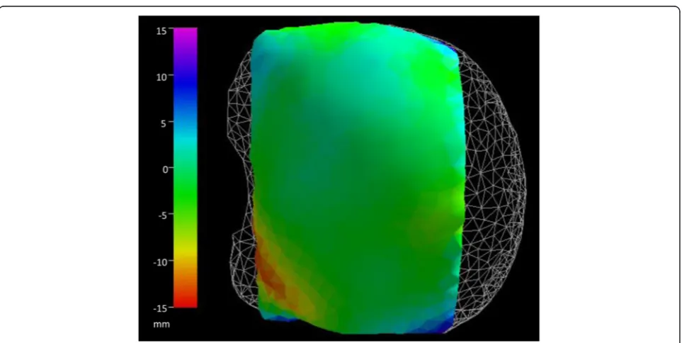
Validation was done by comparing deformation simula-tion and a real ex vivo bovine liver [1]. A compression was made using two horizontal compression paddles in a form similar to the deformation obtained during a mam-mographic examination. The results of this compari-son show a high degree of similarities between the experimental results and the calculated deformations (Fig. 1). The distance between the simulated and the real deformed surface has a standard deviation of about 1 % of the liver length.

The central theme of this paper is to provide a step by step discussion, algorithmic, and actual implemen-tations in the form of working computer routines of the ideas expressed in Costa [1] for fast simulation of biological tissue. In addition, the software for clinical applications is shown, for the first time, by using the program to deform a 3D breast image of a real pa-tient through the use of a 3D scanner in a hospital environment.

Methods

Surface geometry definition

The surface geometry of the objects to be simulated can be derived from data scanned from real data or

from intermediate models. In general, this data is given as a set of surface points (vertex) positions.

For a deformable object, a vector →s_i represents the vertices’ 3D positions, where i enumerates each

ver-tex between 1 and the total number of surface

points N. For the computational code, the x-, y- and

z-components of the vector →s_i are stored in

(X[i], Y[i],Z[i]) and N is stored in the variable NVertex.

The deformation for each vertex can be specified by a displacement vector field →u_i and its x-, y- and z-components are stored in unique column matrix (u[i], u[i+NVertex],u[i+ 2 *NVertex]).

A triangular mesh comprises a set of N′ triangles (in three dimensions) connected by their common vertices and defines the surface shape of an object in 3D solid modeling. To describe each triangle we enumerate three vertices V[1][i], V[2][i], and V[3][i] which must be connected to form a face, similar to

the definition of the WaveFront Object (.obj) File Format [5]. In this case, the index i enumerates each triangle between 1 and the total number of surface triangular faces N’ which in the computational code is stored as NFaces. Note that the V[1][i], V[2][i], and V[3][i] have values between 1 and the total number of surface points N.

Computer routines for faces and vertex areas

The flat nature of triangles makes it simple to deter-mine their normal vector, a three-dimensional vector

A →

i perpendicular to the i-th triangle’s surface. Vector A

→

i can be obtained by calculating the cross product between the vectors that form two edges of the

tri-angle divided by two. Thus the modulus of A→_i is the

area of the triangle. The direction of vector A→_i can be chosen to point outside of the object.

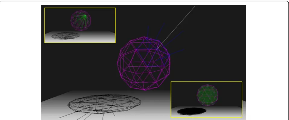
Fig. 2A purple sphere formed by 42 vertices (80 triangles). The blue lines represent the vector area for each triangle neighboring a vertex, for which a blank line represents its resulting vector area. Upper inset: 41 green lines representing the fibers for one vertex. Bottom inset: all superposed fibers (green) for the sphere

Table 1Surface area of objects which the circumscribed sphere (one that touches the polygon at all vertices) has a unitary radius (R=1). The number of verticesNand the number of triangular facesN’are also shown

Object N N’ Analytical Equation Analytical Result _XN

i¼1

S

→

i

XN

′

i¼1

A

→

i

Octahedron 6 8 4pffiffiffi3R2 6.92820 6.92820 6.92820

Icosahedron 12 20 40pffiffi3

5þpffiffi5R

2 _{9.57454 9.57454 9.57454}

The routine below calculates the vector A→_i. The input

variables are vertex vectors →s_i and the vertices of each triangular face: V[1][i], V[2][i], and V[3][i]. On output,

the Cartesian components of the vector A→_i are stored in variables: PerpendicularFaceX[i], PerpendicularFaceY[i] and PerpendicularFaceZ[i], the surface area of each face

represented by the modulus A→_i is stored in variable

PerpendicularFace[i] and faces total area is stored in variable AreaFacesTotal. The faces total area is given by

XN′ i¼1 A

→ i

.

In our method, the deformation of 3D objects is per-formed through the displacement of its vertices. An area vector is assigned to each vertex, in order to determine the force acting over its surface. This area is defined from the area vectors of the triangles (faces) in the vicin-ity of the vertex.

The following routine calculates the auxiliary

variable Shared[i][kk] that stores the identifiers of kk triangles (faces) neighbors to a given vertex i. The

number of neighboring faces of each vertex i is

stored on the output variable NFacesSharingVertex[i].

For example, Shared[25][2]=40, it means that the

face 40 has been identified as the second triangle ad-jacent to the vertex 25and NFacesSharingVertex[25]=3

informs that there are three neighboring faces to the ver-tex 25. The routine has as input variables the vertices V[1][i],V[2][i],andV[3][i]of each triangular face.

Now we can define an area vector →S_i for each vertex as →S_i≡CX

k

!

Ak whereCis normalization constant, i.e. the area vector for a vertex is proportional to the sum of the area vectors of the triangles in the vicinity of the vertex.kvalues in the summation for each vertex i are stored in the variableShared[i][k],wherekvaries from1 to NFacesSharingVertex[i]. Figure 2 illustrates these vectors for the case of a sphere. The triangles that form the surface of a sphere are show in purple. Vectors A→

k are shown as blue lines and S→_i are represented by a white line for one vertex.

The shape of area S→_i is not a triangle in general. But

the sum of the modulus of areas_A→_iorS→_irespectively on

all faces or vertices must be equal to the solid surface area, i.e.

XN′ i¼1 A

→

i

¼XN_i¼1′→S_i¼surface area of the object ð1Þ

Then the area of the verteximust be defined as

S

→

i≡

XN′ i¼1 A

→

i

XN

i¼1

X

kA

→

k

0 B B @

1 C C AXkA

→

k ð2Þ

vector area of faces_A→_i (input) are determined vector

area of each vertex →S_i and the area of the object, stored in variable AreaVertexTotal (outputs).

calculation. The results are the same for at least four signifi-cant figures. Some of these results can be seen in Table 1.

Deformation routine

The general result of the Costa deformation method [1] for fast simulation of biological tissue formed by fibers and fluid can be written as a set of3N +1variables:3N displace-ments u→

1; u

→

2; ⋯;u

→ i;⋯;u

→

N and a variation of internal pres-sureP(stored in variableu[3 *NVertex+ 1]). The approach implements a quasi-static solution for elastic global defor-mations of objects filled with fluid and fibers. The static condition states that the internal force on the surface, due

to all fibersF→

i fibersand the force due to the liquid

F

→

i liquid

¼P S→_i ð3Þ

have a corresponding external force of the same magnitude but in opposite sense at each point of the object surface. The external forces are due to contact forces F→contact or forces resulting from accelerations. For the most common situation the acceleration is due to the gravitational fielda. For this case the pressure is given byρhiawherehiis the vertical component of the distance from the top to the ver-tex iand ρ is the density of the fluid. The result is three equations for each vertex given by

F

→

i fibers

−P S→_i¼F→ i

contact_þρ hiaS

→

i ð4Þ

and one equation for the conservation of volume XN

i¼1S

→

i⋅→ui¼0 ð5Þ

Note that Eq. 5 couples the dislocations (and hence, forces) in perpendicular directions (x, y and z). This coupling creates an effect somewhat similar to the stress and strain tensors in standard elastic theory.

The force due to one fiber connecting vertex i and j obeys Hook’s Law and is proportional to the fiber’s area

(Si+Sj)/2and inverse to its length s

→ i−→sj

, where →s_i and s

→

jare the positions of verticesiand j. The force due to

all fibersF→_ifibersis obtained by connecting each vertexi to other vertices by a set of N-1elastic fibers. These fi-bers are shown as green lines in the upper inset of Fig. 2 for a sphere.

The process of connecting a vertex to other vertices is repeated for each vertex. This meshing strategy for filling the objects superposes fibers during each connection (bottom inset of Fig. 2). Then the superposed volume depends on the mesh discretization. Therefore, a factor N-1 must be included in the denominator in order to maintain Yij a constant value, independent of the

discretization, for bulk fibers:

F

→

i fibers

¼XN_j≠i−Yij SiþSj

u

→

i−→uj

2ðN−1Þ→s_i−→s_j : ð

6Þ

On the other hand, for the surface connections

F

→

i fibers

¼X_k

−γikðSiþSkÞ →u_i−u→ k

2→s_i−→s k

2 ð

7Þ

whereYijandγikare respectively the force per unit of area and length, whose value can be chosen to be Young’s Modulus and superficial tension or their values must be set in a way to fit an experimental deformation result.

These equations can be written as a problem of type A.x = B where B is the column vector defined by the right hand side of Eq. 4 (F→_icontactþρhiaS

→

i) and one extra element equal to zero that imposes the conserva-tion of volume (right hand side of Eq. 5). The left hand sides of Eqs. 4 and 5 define the square matrixA.

The resulting vectorx gives all the displacements and the pressure variation. An example of matricesx, Aand Bcan be seen in Eq. 8.

Border conditions

The degenerate first mode, corresponding to the zero eigenvalue, represents a rigid body translation because, although moving, each vertex is stationary relative to the other. Of course, the presence or absence of this degen-erate mode will not influence the purely deformable characteristics of the system. This degeneracy can be re-moved using boundary condition.

For boundary condition some vertices can be considered fixed to an external support. To achieve this condition, verteximust not move, or moves a negligible amount com-pared to the movement of the others vertices. The resulting movementxiof the vertex is controlled by the size of

elem-entAii, because each element of the product of matrices A

andxis naturally expressed as the sum ofNproductsAijxj.

In order to impose the border conditions, i.e., make xi<<xj,

the elementAiishould be done much bigger than the other

elementsAijin lineiof matrixA. An example of this

pro-cedure can be seen in section "An example for a rectangle".

Computer routines for general 3D objects

We need to create a matrix A[1..3N+1] [1..3N+1]as the input matrix of equationA.x=B. A large number of ele-ments in matrix A in general vanish. Thus we initialize by writing zeros in all elements of this matrix.

For a deformable object the triangles’positions and shapes change. Therefore, we need to recalculate the perpendicular of each triangle and vertex at each calculation step.

input data, stored in the variables Yx, Yy and Yz(Young’s

modulus) and gamma (superficial tension). Then, the A matrix (output) is determined from the quantities

We need to create B[1..3N+1]as the input containing the right-hand side of equation A.x =B. As the routine input data has the following constants: the applied force is stored in the variable Force, the product gravitational field and the density of the liquid is stored in the vari-ablegd; and the number of the vertex where force is ap-plied is stored in the variablemove. So, we implemented the right side of Eq. 4, creating the vectorB.

Concave objects

Note that all fibers effectively exist for a convex ob-ject. However for a concave object, some fibers con-nect pairs of vertices beyond the surface of the object, so these fibers do not actually exist. In order to consider this situation, forces due to fibers need to be removed when they pass through the surface.

Then the number N is equal to the number of

vertices only for the convex object. For concave

ob-ject, N must be equal to the number of effective

connections.

Two tests must be done in order to detect the fi-bers that pass through the surface of the object. First, we need to test if the fiber starting at vertex i goes inside or outside the object. Then, we calculated the scalar product for all k triangles neighboring the

ver-tex i: A→ k⋅ S

→ i−S

→ j

. If there is any negative result, the

fiber connecting the vertices i and j goes outside the object and the matrix element Aij must be set equal

to zero.

A second test is needed because if a fiber intersects any triangle, it goes outside the object. Then we used the fast 3D line segment-triangle intersection test de-veloped by Chirkov [6]. If a fiber that connects the vertices i and j intersects any triangle, the matrix element Aij also must vanish. In this link [7] there is

an executable beta version of our software with this and other functionalities.

The matrix solution

To simulate a non-linear stress–strain relation the value of Yij can be defined as a function of the

dis-placement u→_i−→u_j in the last step. Shortly after each increment of deformation, the element geometry and stiffness value is updated to model the nonlinear be-havior of the material. The variation of external force on each interaction should be chosen to obtain the desired precision or an acceptable calculation time. Therefore, in this case, matrix A must be recalculated at each step.

But for situations where the area →S_i and the distance

of each vertex →s_i−→s_j varies in a negligible amount on

the left hand side of Eqs. 4 and 5 and the elasticity is lin-ear (surface tension γik and Young’s Modulus Yij are

constants independent of the deformation), matrix A is constant and can be operated once. For example, LU de-composition from the book Numerical Recipes in C [8] was used to solve the problem A.x=B. If matrix A is constant, the routine given in this book allows LU de-composition result to be left in place for successive calls with different right-hand sidesBto achieve a greatly re-duced calculation time.

Results and discussions An example for a rectangle

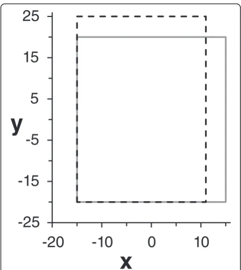
Let us consider the problem of a rectangle with edges ± 15î± 20ĵthat defines the four vertices→s_i(Fig. 3). For this first example, the units are arbitrary and simplicity sur-face tension effects are not taken into account. In this caseN=N’=4 and the“areas”Ai in this two-dimensional

case are actually the edges of length30and40. Each vertex has two neighbors, one in x direction and another in the

directiony. Then using Eq. 1 and 2 we obtain that→S_i¼7

4^i3^j

and→S_i¼35.

For simplicity, the 2D Young’s Modulus is set to be a constantYij=360and no acceleration effect is taken into

account. The boundary conditions are chosen to be as least restrictive as possible: the lower left corner is fixed, the lower right corner is constrained to move only hori-zontally. In order to obtain these boundary conditions, we make the matrix elementsAiilarge, equal to 109, for

these vertices in these directions.

Forces of equal magnitudeFicontact=1680 are applied to

the upper corners vertically upward. Using Eq. 4 and 5 for this rectangle, we can write the problemA.x=Bas:

Fig. 3Un-deformed rectangle is shown in solid line. The lower left corner is fixed, the lower right corner is constrained to move only horizontally. The dashed line shows the new shape after forces (numeric of 1680) are applied to the upper corners vertically upward

329 −105 −84 −140 0 0 0 0 28

−105 329 −140 −84 0 0 0 0 28

−84 −140 109 _{−105 0 0 0 0 −28}

−140 −84 −105 329 0 0 0 0 −28

0 0 0 0 329 −105 −84 −140 21 0 0 0 0 −105 109 _{−140 −84 −21}

0 0 0 0 −84 −140 109 _{−105 −21}

0 0 0 0 −140 −84 −105 329 21 28 28 −28 −28 21 −21 −21 21 0

2 6 6 6 6 6 6 6 6 6 6 6 6 4 3 7 7 7 7 7 7 7 7 7 7 7 7 5

u1x

u2x

u3x

u4x

u1y

u2y

u3y

u4y

P 2 6 6 6 6 6 6 6 6 6 6 6 4 3 7 7 7 7 7 7 7 7 7 7 7 5 ¼ 0 0 0 0 1680 0 0 1680 0 2 6 6 6 6 6 6 6 6 6 6 6 4 3 7 7 7 7 7 7 7 7 7 7 7 5

ð8Þ

Solving this matrix equation foruwe obtain the dislo-cations that should be added to the vertices position to get the new deformed shape. The result for the position of the right corners is sx=11 and for the upper corners

sy=25, as shown in Fig. 3. Other examples for 3D objects

are shown above.

An example for a sphere

Let us now consider that a sphere with a radius of one meter. The border conditions impose that all upper ver-tices, defining a spherical cap of height 0.2, cannot move. The parameters are defined as: the surface tension γik and Young’s ModulusYijare adjusted to be equal to

3 with units in kNewtons and meters; the acceleration due to gravity is acting down and increases at each iter-ation 1 m/s2in a total of ten steps until the final value

g=10 m/s2is reached; the matrixAis constant; the num-ber of vertices isN=162; and the density of the fluid isρ = 1000 kg/m3. To show the effect of contact forces

F →

contact , at the final step a force →F¼−300 ^iþ^jþ^k

is applied to the vertex number1.

Inside the link [9], we provide a complete source code for a deformable 3D sphere. The result of this code can be seen in Fig. 4.

The ideas given by Wright [10] were used to draw the objects and shadows. In addition, the routine to make spheres was taken from Shreiner [11].

An example for a real in vivo breast

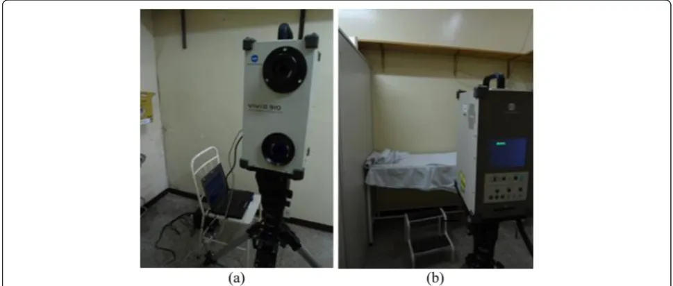
In order to show the benefit of our software for clinical applications, we used our computer program to deform 3D breasts images, acquired from a set of four patients in a real hospital environment. The 3D geometries of the breasts’surfaces were obtained using a non-contact 3D Digitizer Konica Minolta Vivid 910, as shown in Fig. 5.

Reconstruction was made by merging different views of the patients in a standing position taken from differ-ent angles. Several reference points were located on each patient, in order for an accurate merge. These images were mapped and the final reconstruction can be seen in Fig. 6. These surfaces were exported in obj format and run through our simulator.

The tissues were simulated as isotropic and linear, allowing us to do LU decomposition of the matrix A only once before the first iteration. Thus, for each inter-action the right hand of Eq. 4 (vectorB) are updated and

new values for hi; aandS →

i must be incorporated at the

next calculation step. We choose this procedure because, according to Costa [1], the resultant deformation in this case is similar to the deformation of the slower procedure that repeats LU decomposition at each interaction

(updat-ing→S_iand→r_i−→r_j).

Nevertheless, for nonlinear approaches the matrix A changes for each step and it must be recalculated for each iteration, imposing the necessity of the

slower method. An example of a nonlinear elasticity is shown in Costa [1].

Best accuracy is expected if small steps are used (great number of interactions), since in this case the variation of hi; aandS

→

iis smaller and the outcome get closer to the continuous (analytical) result.

We chose the surface tension γik= 48 MN/m, the

Young’s Modulus Yij= 48 kPa and the density of the

fluid ρ= 1000 kg/m3. The boundary conditions in the

Fig. 7The breast surface with 402 triangles (purple) and the simulated fibers set (green) for patient number four

case of breast deformation are the chest region that re-strains the tissue movement in any direction.

Figure 7 shows the result for patient number four. The surface of the breast is formed by 402 faces and the sim-ulated fibers are also shown.

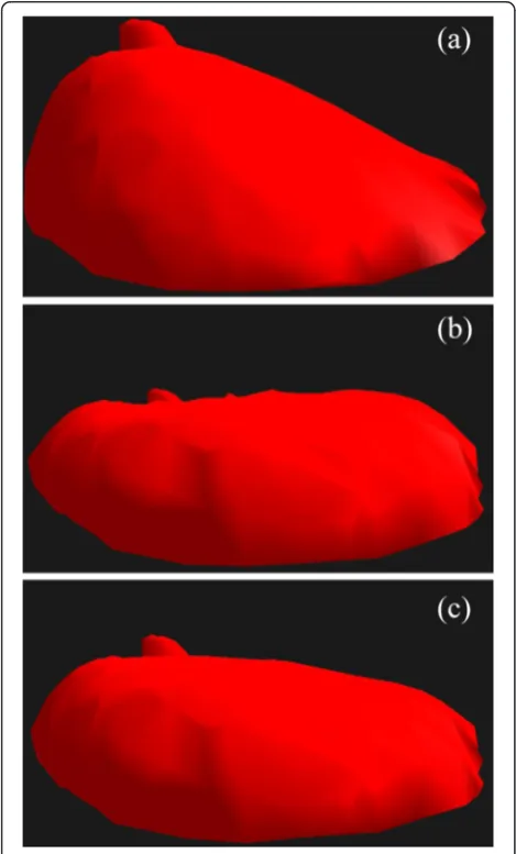
A compression, perpendicular to the chest plane, was set to the simulated breasts due to the increase of the gravitational field (10 m/s2). The number of steps n to achieve the final gravitational field value could vary. The uncompressed (a) and compressed breast shape for the number of steps n equal to one (b) and 100 (c) are shown in Fig. 8 for patient number four.

Finally, we decompressed the breast by decreasing the acceleration applied to the deformed breast until the acceleration vanished. The same number of steps used during the compression procedure was used for the decompression. Then the mean difference in the

initial (uncompressed) and final (decompressed) nodes position was calculated as:

XN i¼1 u

→

i

N

ffiffiffiffiffiffiffiffiffiffiffiffiffiffiffiffiffiffiffiffiffiffiffiffiffiffiffiffiffiffiffiffiffiffiffiffiffiffiffiffiffiffiffiffiffiffiffiffiffiffiffiffiffiffiffiffiffiffiffiffiffiffiffiffiffiffiffiffiffiffiffiffiffiffiffiffiffiffiffiffiffiffiffiffiffiffiffi

smax x −sminx

2_þ

smax y −sminy

2

þ smax

z −sminz

2

r ð9Þ

where sxmax and sxmin are the maximum and minimum values ofsx(the same for the directionsyandz).

For a continuous (analytical) approach, no difference on uncompressed and decompressed position are ex-pected, and the result of Eq. 9 must be zero. For a nu-merical (discrete) approach differences on the initial and final position are expected due to errors introduced in the calculation of matrixBin each step. However, in our algorithm the results of Eq. 9 are small; numerically3 % for 1 interaction and decreased to about 0.3% and 0.03 %for10and 100interactions, respectively. And the method evaluation results were similar for all four pa-tients. These results demonstrate a good algorithmic be-havior for the complete compression and decompression process of the breasts.

Conclusions

This work presents the implementation of a new general approach for modeling soft tissue compression process. The method was successfully applied to compress a 3D breast model from real patients.

The fast simulation of deformation of biomaterial using this algorithm could provide more realistic images that could serve for educational, clinical application, and research purposes. The latter include investigations of different breast imaging techniques involving com-pressed and uncomcom-pressed breasts.

Competing interests

The authors declare that they have no competing interests.

Authors’contributions

AGOS and CNRO carried out the clinical breast scanner procedures and managed the ethical committee documentation and its approval. AGOS also performed the breast image reconstruction merging different scanned views. AM participated in the design of the study, organized the figures and helped to draft the manuscript. IFC drafted the manuscript, conceived of the study, participated in its design and coordination. All authors read and approved the final manuscript.

Acknowledgments

The authors gratefully acknowledge the University of Brasilia and the financial support from the Brazilian science agency (CNPq) through research project 474831/2012-4.

Author details

1_{Faculdade UnB Planaltina, University of Brasilia, 70919-970 Brasilia, DF, Brazil.} 2

Medicine Department, University of Brasilia, 70919-970 Brasilia, DF, Brazil.

Received: 10 December 2014 Accepted: 31 March 2016

References

1. Costa IF. A novel deformation method for fast simulation of biological tissue formed by fibers and fluid. Med Image Anal. 2012;16:1038–46. 2. Meier U, López O, Monserrat C, Juan MC, Alcañiz M. Real-time deformable

models for surgery simulation: a survey. Comput Methods Prog Biomed. 2005;77:183_–97.

3. Basdogan C, Sedef M, Harders M, Wesarg S. VR-based simulators for training in minimally invasive surgery. IEEE Comput Graph Appl. 2007;27:54–66. 4. Filho PJ, Sousa EAC. Reconstruction and mesh generation in

three-dimensional biomechanical structures for finite elements analysis. Braz J Biom Eng. 2009;25(1):15–20.

5. McHenry K, Peter B. An overview of 3d data content, file formats and viewers, National Center for Supercomputing Applications. 2008. p. 1205. 6. Chirkov N. Fast 3D Line Segment_—Triangle Intersection Test. J Graph Tool.

2005;10(3):13–8.

7. Costa IF. Authors’own website. https://www.sites.google.com/site/unbivan/ download. Accessed 12 April 2016.

8. Press WH, et al. Numerical Recipes in C: the art scientific computing, 2th edn. Cambridge: Cambridge University Press; 1992. (Chapter 2.3 - LU Decomposition and Its Applications)

9. Costa IF. Authors’own website. https://sites.google.com/site/unbivan/FFM. cpp. Accessed 12 April 2016.

10. Wright R, Sweet M. OpenGL SuperBible. 2nd ed. Essex: Pearson Education; 1999 (Chapter 9–Lighting and Lamps).

11. Shreiner D. OpenGL programming guide: the official guide to learning OpenGL, versions 3.0 and 3.1. 7th ed. Boston: Addison-Wesley; 2009. Chapter 2 - State Management and Drawing Geometric Objects.

• We accept pre-submission inquiries

• Our selector tool helps you to find the most relevant journal • We provide round the clock customer support

• Convenient online submission • Thorough peer review

• Inclusion in PubMed and all major indexing services • Maximum visibility for your research

Submit your manuscript at www.biomedcentral.com/submit