Development of an algorithm for evaluating the impact of measurement variability on response categorization in oncology trials

R E S E A R C H A R T I C L E

Open Access

Development of an algorithm for

evaluating the impact of measurement

variability on response categorization in

oncology trials

Jeong-Hwa Yoon

, Soon Ho Yoon

and Seokyung Hahn

Abstract

Background:Radiologic assessments of baseline and post-treatment tumor burden are subject to measurement variability, but the impact of this variability on the objective response rate (ORR) and progression rate in specific trials has been unpredictable on a practical level. In this study, we aimed to develop an algorithm for evaluating the quantitative impact of measurement variability on the ORR and progression rate.

Methods:First, we devised a hierarchical model for estimating the distribution of measurement variability using a clinical trial dataset of computed tomography scans. Next, a simulation method was used to calculate the probability representing the effect of measurement errors on categorical diagnoses in various scenarios using the estimated distribution. Based on the probabilities derived from the simulation, we developed an algorithm to evaluate the reliability of an ORR (or progression rate) (i.e., the variation in the assessed rate) by generating a 95% central range of ORR (or progression rate) results if a reassessment was performed. Finally, we performed validation using an external dataset. In the validation of the estimated distribution of measurement variability, the coverage level was calculated as the proportion of the 95% central ranges of hypothetical second readings that covered the actual burden sizes. In the validation of the evaluation algorithm, for 100 resampled datasets, the coverage level was calculated as the proportion of the 95% central ranges of ORR results that covered the ORR from a real second assessment.

Results:We built a web tool for implementing the algorithm (publicly available athttp://studyanalysis2017. pythonanywhere.com/). In the validation of the estimated distribution and the algorithm, the coverage levels were 93 and 100%, respectively.

Conclusions:The validation exercise using an external dataset demonstrated the adequacy of the statistical model and the utility of the developed algorithm. Quantification of variation in the ORR and progression rate due to potential measurement variability is essential and will help inform decisions made on the basis of trial data.

Keywords:RECIST, Measurement variability, Hierarchical model, Algorithm

© The Author(s). 2019Open AccessThis article is distributed under the terms of the Creative Commons Attribution 4.0 International License (http://creativecommons.org/licenses/by/4.0/), which permits unrestricted use, distribution, and reproduction in any medium, provided you give appropriate credit to the original author(s) and the source, provide a link to the Creative Commons license, and indicate if changes were made. The Creative Commons Public Domain Dedication waiver (http://creativecommons.org/publicdomain/zero/1.0/) applies to the data made available in this article, unless otherwise stated. * Correspondence:[email protected]

†_{Jeong-Hwa Yoon and Soon Ho Yoon contributed equally to this work.}

3_{Medical Statistics Laboratory, Department of Medicine, Seoul National}

University College of Medicine, 103 Daehak-ro, Jongno-gu, Seoul 03080, South Korea

Background

In medicine, some diagnoses of diseases or determina-tions of treatment response are dichotomized or catego-rized according to changes in continuous data as measured before and after intervention. In oncology, treatment response after anti-cancer therapy is deter-mined based on the percent change of the tumor burden before and after the treatment, as measured by physi-cians on computed tomography (CT) scans. The tumor burden in a patient is represented by measurements of representative lesions (so-called target lesions), followed by the sum of the measurements. The objective response rate (ORR) and progression rate, which are used in on-cology trials, are imaging-based measures of outcomes assessed using the Response Evaluation Criteria in Solid Tumors (RECIST) response categorization according to the percent change of the tumor burden before and after treatment [1]. The categories include complete response, partial response, stable disease, and progression. The ORR and progression rate are defined as the percentage of patients who achieve complete or partial response and progression, respectively [2].

Radiologic measurements of the tumor burden can be inconsistent across assessments, which may affect the assessed percent change of the tumor burden, the re-sponse categorization, and the resulting ORR and pro-gression rate [3]. Indeed, it has been suggested that reimaging the same single-tumor burden can result in an increase or decrease of the burden size by less than 10% relative to the first measurement [4], and that when different readers assess the same single-tumor burden before and after treatment, the absolute difference in the values of percent change (%) between readers can be as much as 30% [5]. This measurement variability eventu-ally results in variability in the response classification and ORR [6].

Many oncology trials designate the objective response as a primary or a secondary outcome and provide the ORR as a measure of the outcome, but the reliability of RECIST-based response determinations and the ORR due to measurement variability in oncology trials re-mains poorly understood [5]. In this study, we developed an algorithm for quantitative evaluation of the impact of measurement variability on the ORR and progression rate, which is an area that has not yet been considered in previous research.

The RECIST-based response could be considered as an ordinal measure. Some statistical methods for assessing the agreement of such ordinal data have been suggested in the literature [7–10]. The response categorization is an or-dinal dichotomization of change in tumor burden. Follow-ing the RECIST guideline, the tumor burden is essentially calculated by summing the measurements of the various target lesions that can adequately represent the overall

tumor burden in a patient. Since measurement error fun-damentally occurs when observing lesion sizes, and mani-fests as measurement variability of tumor burden size, percent change, and response categorization, it is import-ant to understand the primary behavior of measurement variability by modeling measurements of lesion size. The response categorization of tumor burdens of various sizes initially determined to have shown the same response can in fact be differently reproducible based on how or whether the measured size of the tumor burdens is close to the cutoff values for categorization. Such differences should also be taken into account for measuring the un-certainty and reproducibility of the eventual RECIST-based response.

Bland and Altman (1986 and 1999) originally pro-posed the limits-of-agreement (LOA) method for assessing agreement between measurements by two observers [11, 12]. LOAs provide a straightforward way of evaluating measurement agreement by plotting the measurement difference against the mean of the two measurements. Sometimes the differences be-tween the measurements are dependent on the size of the measurements, with increasing measurement error accompanying an increasing scale of the measurement values, in which case conventional LOAs may not rep-resent the data well. When a distribution of errors is skewed, data are often log-transformed to approximate normality. Euser et al. (2008) discussed a modeling approach to calculate meaningful LOAs on log-trans-formed data [13].

adequately predicted the actual repeatedly read measure-ments and whether the resulting ORR replicated the ORR as assessed by actual third parties.

This article is organized as follows. The Methods sec-tion first introduces the data structure and describes the process of the development of the evaluation algorithm by modeling and simulations, followed by the method of validation. The Results section explains the routines of the developed web tool for implementing the algorithm and interprets the results of the validations. The final section contains a discussion of the usefulness and limi-tations of our method and the usability and potential of the algorithm.

Methods

RECIST guideline

The RECIST guideline is a set of standardized criteria for assessing tumor response after anti-cancer treatment in oncology trials. The guideline mainly deals with how to define a tumor burden, how to measure changes of tumor burden, and how to categorize the response of the tumor after treatment. Following the guideline, the tumor burden is calculated by summing the measure-ments of the various target lesions that can adequately represent the overall tumor burden in a patient. The percent change is then calculated as a change in the tumor burden after treatment relative to its baseline value as a percentage. The RECIST-based response is fi-nally categorized based on the percent change of the tumor burden. The categories include complete response (−100%), partial response (−30% or less), stable disease (−30 to 20%), and progression (20% or more).

Data

In order to estimate the distribution of measurement errors through modeling and to develop an algorithm to evaluate the impact of measurement variability on re-sponse categorization in oncology, we constructed a dataset by obtaining repeated evaluations of the selected lesions before and after treatment, thereby enabling esti-mation of the within-lesion component of the measure-ment variability.

De-identified chest CT scans were initially obtained from 75 patients who were enrolled in an existing phase III ran-domized trial of chemotherapy for advanced small-cell lung cancer (SCLC). A single radiologist chose a total of 249 measurable target lesions in the 75 patients, and the me-dian number of measurable target lesions per patient was 3. Each target lesion was read by six radiologists in four separ-ate sessions, twice at baseline and twice after treatment.

Twenty-four measurements of the longest diameter (12 at baseline and 12 at follow-up) were taken from each lesion. Of all the target lesions, 119 were on lymph nodes. A short-axis diameter, perpendicular to the

longest diameter, was additionally taken from those target lymph nodes. Twenty-four measurements of the shortest diameter (12 at baseline and 12 at follow-up) were taken from each lymph node.

For validation of the estimated distributions of meas-urement error and the evaluation algorithm, we used an-other dataset of 56 target lesions from 22 patients with refractory SCLC from a phase II trial. Each target lesion was measured by a within-trial local reader and one ex-ternal reader in two separate sessions, once at baseline and once after treatment. The longest diameters and short-axis diameters were taken from the solid lesions and lymph nodes, respectively.

Modeling

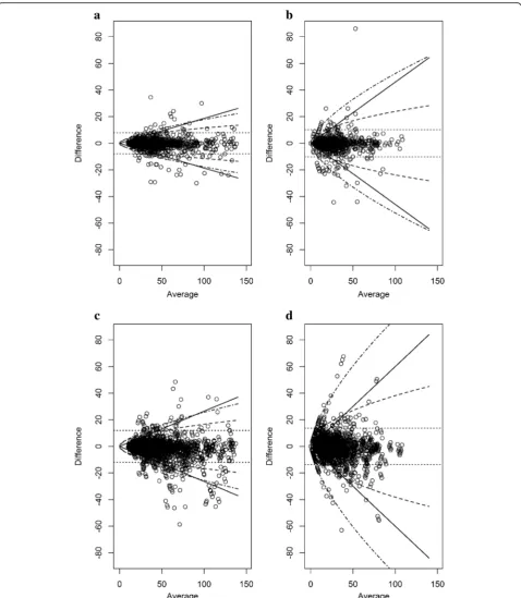
A hierarchical linear mixed-effects model including le-sions, readers, and the interaction effects of lesions and readers as random effects was considered based on the measurements obtained from the six reviewers at each of the baseline and the post-treatment phases [14]. We assessed the plausibility of using the square root, cube root, and log transformation of the lesion size as possible assumptions for the distribution of measurement errors. LOA presentations with a Bland-Altman plot [11] were explored at each phase (Fig. 1) (see formulas of the LOAs on the original scale for thenth root-transformed variables in Additional file 1). Since the LOA from the square root transformation of the lesion size described the data pattern appropriately, we chose the square root transformation, considering the nonlinear lesion size-dependency of the measurement error. We trimmed off 5% of the outlying data with a large standardized re-sidual based on the considered model using the trans-formation at each phase [15].

The final model was then fitted in a bivariate form, ac-counting for a possible correlation between the measure-ments in the baseline and the post-treatment phases:_{ffiffiffiffiffiffiffiffiffiffi}

Yijk:b

p ffiffiffiffiffiffiffiffiffiffi Yijk:p

p

= μ_μb

p +

αi:b

αi:p

+ β_βj:b j:p

+ γ_γij:b ij:p

+

εðijÞk:b

εðijÞk:p

, where

ffiffiffiffiffiffiffiffiffiffi Yijk:b

p ffiffiffiffiffiffiffiffiffiffi Yijk:p

p

denotes the square

root-transformed measures of the lesion diameters at baseline and post-treatment (b: baseline, p: post−

treatment) and μ_μb

p are the fixed parameters. In

addition, α_αi:b i:p

, the lesion effect, β_βj:b j:p

, the reader

effect, and γ_γij:b ij:p

, the interaction between the lesion

and reader, are random effects normally distributed with

a mean vector of 0

matrices of σα:b 2_{; σ}

α:b;p

σα:b;p; σα:p2

, σβ:b 2_{; σ}

β:b;p

σβ:b;p; σβ:p2

and

σγ:b2; σγ:b;p

σγ:b;p; σγ:p2

, respectively. The residual error term

εðijÞk:b

εðijÞk:p

with a mean vector of 0

0 and a

variance-covariance matrix of σε:b 2_{; σ}

ε:b;p

σε:b;p; σε:p2

indicates

the intra-reader measurement error given a lesion and a reader [16]. The inter-reader measurement error followed a normal distribution with a mean vector of

0

0 and a variance-covariance matrix of

σβ:b2þσγ:b2þσε:b

2

2 ; σβ:b;pþσγ:b;pþ σε:b;p

2

σβ:b;pþσγ:b;pþσε₂:b;p; σβ:p2þσγ:p2þσε:p

2

2

!

; as

calcu-lated by the variance-covariance component estimates of random effects and residuals to represent deviation in measurements by several readers [13]. Posterior distribu-tions of the variance-covariance components, the param-eters of random effects, and the residual errors were obtained using the Markov-chain Monte Carlo method in a Bayesian framework with non-informative priors [17]. Modeling was performed separately for the longest-diameter data and the shortest-longest-diameter data. The modeling process was run in the software R [18].

Simulation

We simulated a situation in which the baseline and post-treatment diameters of a tumor burden observed in the first reading were re-measured by the same reader or another reader in order to obtain the probability that the change would be classified as a certain tumor re-sponse from the re-measured tumor burden sizes. In order to facilitate the simulation, we established artificial datasets of the observed tumor burden sizes and their hypothetical second measurement values using the esti-mated distributions of intra- or inter-measurement errors. These datasets were used to calculate the prob-ability that the second measurement would be desig-nated as a certain tumor response. This was performed repeatedly for various scenarios. The simulation process was as follows:

(a) Construction of an artificial dataset of 100 tumor burdens with the same number of target lesions:

When the tumor burden had a single target lesion (n= 1), we let Yb1 and Yp1 be the baseline size and

post-treatment size of a lesion, respectively. The lesion size itself became the tumor burden. If we assume that acpercent change of the tumor burden occurred, then

Yp1 is equal toYb1þcYb1.

When there was a set of tumor burdens having two or more target lesions (n≥2), we let Ybx and Ypx be the corresponding baseline size and post-treatment size of the x thlesion in a tumor burden and let Pn_x¼1Ybx and

Pn

x¼1Ypx therefore correspond to the baseline and post-treatment tumor burden, respectively. If we assume that ac percent change of the tumor burden occurred, then

Pn

x¼1Ypx is equal to

Pn

x¼1YbxþcPnx¼1Ybx. The sizes of the lesions in each of the 100 tumor burdens at baseline were generated from a log-normal distribution acquired empirically from the lesion sizes in the original dataset [19]. Because the target lesions within a tumor burden do not change uniformly after treatment, the percent change (c_x) of the xthlesion in a tumor burden was ran-domly determined from a normal distribution with a mean of c and a certain variance, with the restriction that Pn_x¼1cxYbx was equal to cPnx¼1Ybx. The estimated variances using tumor burdens with multiple target le-sions from the longest-diameter data and the short-axis diameter data were 0.17 and 0.10, respectively.

(b) Generation of hypothetical second assessments in the baseline and post-treatment phases:

We generated measurement errors ðϵbx;ϵpxÞ of thex th

lesion in a burden in the two phases together using the distribution estimated in the previous modeling step. We squared the sum of the square root of the first measurement value produced at (a) and the error at each phase to generate the hypothetical second measurement values of the xthlesions, ðð ffiffiffiffiffiffiffiYbx

p

þϵbxÞ 2

;ðpffiffiffiffiffiffiffiYp_xþϵp_xÞ2Þ

¼ ðY0

bx;Y0pxÞ. For all lesions in a tumor burden, the above procedure was performed to produce the hypo-thetical second assessments of the burden, Pn_x¼1Ybx0 andPn_x¼1Ypx0.

(c) Calculation of the probability of designating a certain tumor response at the second assessment for a given first assessment:

We estimated the probabilities as proportions that the simulated percent changes would be designated as an objective response (i.e., complete or partial

response), P½

Pn x¼1Ypx0−

Pn x¼1Ybx0

Pn x¼1Ybx0

≤−0:3; or progression ;

P½

Pn x¼1Ypx0−

Pn x¼1Ybx0

Pn x¼1Ybx0

≥0:2.

(d) Producing medians of the probability:

posterior distributions of the variance-covariance com-ponent parameters to produce the medians of the esti-mated probabilities for specific designations.

(e) Performing the above simulation processes for different scenarios:

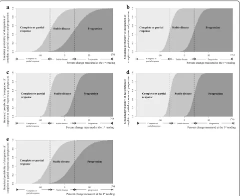
A series of simulation processes was performed for various scenarios, assuming the following factors: differ-ent numbers of target lesions (1≤n≤5) and different constitutions of the solid lesions (long-axis diameter, up to 5) and lymph nodes (short-axis diameter, up to 2) in the tumor burden; various baseline sizes of the lesion diameter when a single target lesion (n= 1) was consid-ered (the ranges of the long- and short-axis diameters were 10–150 mm and 10–80 mm, respectively, and the intervals were 1 mm); different percent changes, − 1.0≤c≤1.0 (the interval was 0.01); and within-reader variability or between-reader variability. The distribu-tion of the measurement error was set according to whether a single reader or multiple readers reassessed the lesion size and whether the target lesion was a solid lesion or lymph node. The resulting probability curves from the simulations are exemplified in Fig. 2

for five specific scenarios, with each curve represent-ing the probability for each categorization dependrepresent-ing on the scale of percent change measured upon the sec-ond assessment.

The above simulation processes were conducted in R software [18].

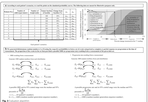
Evaluation algorithm

A diagram of the algorithm is shown in Fig.3. The algo-rithm to evaluate the impact of measurement variability on the ORR at the level of a trial features the probabil-ities calculated in the simulation step. For the trial data of each patient, the probability that the patient’s tumor burden with a reported percent change would be desig-nated as a complete or partial response in a hypothetical reassessment can be obtained (step (a) in Fig. 3). The event that a complete or partial response was declared at the second assessment was a random variable from a Bernoulli distribution with the respective probability. From the given data, we generated dichotomous random numbers (1 or 0) using the corresponding probabilities to form a set of events for determinations of complete or partial response at the time of reassessment (step (b) in Fig. 3). The proportion of the events in the set then provided a possible ORR resulting from a reassessment of the given dataset. By repeating the trial 1000 times, a range of simulated results was produced, with a 95% central range of ORRs determined in the reassessment.

The reliability of the progression rate can be assessed in the same way. However, if patients experience unequivocal

radiologic progression, symptomatic progression, or death, a definitive probability of 1 is assigned for progression at the second assessment, as such cases are not affected by measurement variability.

This algorithm was implemented on a website using the Python programming language (Python Software Foundation,https://www.python.org/) [20].

Validation of the evaluation algorithm using a real dataset

In order to validate the estimated distribution of meas-urement error from modeling, for each tumor burden in the validation dataset, we calculated the 95% central range of hypothetical results of the second readings. The coverage level was calculated as the proportion of the 95% central ranges that covered the actual burden sizes measured by the second radiologist. For the validation dataset, we produced the 95% central range of simulated ORRs that we could expect from a reassessment using the evaluation tool. We repeated this process using 100 sampled datasets drawn by random sampling with re-placement from the original dataset, and the coverage level was calculated as the proportion of the 95% central ranges that covered the actually observed ORRs from the second reading. We considered that a coverage level close to 95% was indicative of validity [21].

Simulation studies

To investigate the impact of different characteristics of data on the reproducibility of trial results, we generated sets of 50 solid tumor burdens at baseline and post-treatment with different characteristics. For simpli-city, we only considered single target lesions (i.e., that the tumor burden was the lesion size). Simulation fac-tors were considered for different observed ORR results, different sizes of tumor burden at baseline, and different patterns of the resulting percent change after treatment. We plotted the 95% confidence interval (CI) of the served ORR and the 95% central range of ORRs ob-tained from re-assessment by a different observer for each combination of characteristics.

Results

Demonstration of the web tool

An algorithm for calculating the 95% central range of expected ORRs (or progression rates) in a repeated trial was developed, and it is available online as a web tool (http://studyanalysis2017.pythonanywhere.com/). For usage of the tool, a dataset containing the patient ID, organ information (solid organ or lymph node), le-sion size at baseline, and lele-sion size at post-treatment should be uploaded, and further information about the dataset should be added, including the study name, treatment name, and the number of enrolled patients with unequivocal radiologic progression, symptomatic

progression, or death. On the webpage, the uploaded data are confirmed and processed, yielding the num-ber of solid organ tumors, the numnum-ber of lymph nodes, the percent change (%), the tumor burden at baseline (mm), and the tumor burden at post-treat-ment (mm). According to whether the same or an-other radiologist were to reassess the tumor response, the probability of being diagnosed with a complete or partial response (or progression) upon a reassessment of each patient is presented (Fig.4(a)). Finally, the 95% central range of the ORRs and 95% central range of the progression rates determined in the reassessment are shown (Fig.4(b)).

a

b

c

e

d

Validation results of the estimated distributions of measurement errors and the evaluation algorithm

In the validation of the estimated distribution of measure-ment errors, the actual second measuremeasure-ment value was located within the 95% central range of the hypothetical second readings in 19 of 22 and 20 of 20 burdens at base-line and post-treatment, respectively (Fig.5(a)). Therefore, the coverage level was 93%. Concerning the results of the validation of the evaluation algorithm, for the 100 resampled datasets, the ORR resulting from a real second assessment lay in the 95% central range of simulated ORRs in all datasets (Fig.5(b)). The coverage level was 100%.

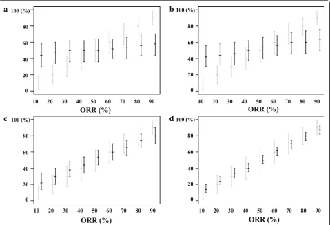
Simulation studies

For the trial data with a smaller lesion size at baseline, the 95% central ranges of the re-assessed ORRs tended to be wider ((a) versus (b) and (c) versus (d) in Fig. 6). For the trial data where the occurred percent changes of tumor burdens were distributed closely around the re-sponse cutoff value of −30%, the 95% central ranges of the re-assessed ORRs tended to be wider, and did not coincide with the 95% CI in many cases apart from when the observed ORRs were close to 50% ((a) versus (c) and (b) versus (d) in Fig. 6). High reproducibility was ob-served when the baseline lesion size was large and the

occurred percent changes were distributed largely away from the cutoff value (Fig.6(d)).

The second set of simulation studies also showed a similar pattern (Additional file2: Figure S1, Additional file3: Figure S2, and Additional file 4: Figure S3). The 95% CIs tended to coincide well with the 95% central ranges of the re-assessed results of ORRs when the assumed true ORR was 50%, regardless of the baseline burden sizes and per-cent changes. When the assumed ORRs were smaller or greater than 50% by a difference of 30%, the tendency for overlap depended on the distribution of percent changes, and in particular how closely they were aggregated to the cutoff. When the percent changes were distributed closely to −30%, the degree of overlap was small, indicating that the data were very vulnerable to measurement variability in assessing tumor response. When every other condition was fixed, larger baseline burden sizes resulted in larger overlap. Whether the 95% central range covered a point estimate of ORR also demonstrated a similar pattern.

Discussion

In oncology, treatment response is determined based on radiologic assessments of the tumor burden, which are subject to measurement variability. It has not been pos-sible to assess the degree to which the resulting ORRs

a

b

and progression rate in specific trials are robust against measurement variability. In this study, we developed an algorithm for quantifying the impact of measurement variability on the ORR and progression rate from a specific trial, as well as a web tool for implementing the algorithm. We presented the sequence of steps used to develop the algorithm, including a method of modeling measurement error, a method of calculating the prob-ability representing the effect of measurement error on determination of treatment response, and the process of applying the final algorithm to evaluate the impact of measurement variability on the results from a trial.

Our hierarchical linear mixed model was constructed with the goal of estimating the variance components capturing measurement variability as the remaining

variation after accounting for other specific sources of variation. Although the data structure suggested that lesions were nested with patients, because the variation among the patient-specific measurements was in fact part of the variation of the lesion-specific measurements, it was unnecessary to separate these in the model be-cause this nesting did not influence the remaining varia-tions. The estimated distributions of intra-reader and inter-reader measurement errors did not change de-pending on whether or not the patient effect was added to the model.

inherent characteristics of a lesion would have a similar effect on measurement errors at baseline and at post-treatment. We thus used a bivariate mixed-effects model to account for the correlation between measurement errors before and after treatment.

There was a small proportion of outlying data ob-served in LOAs presented with a Bland-Altman plot. By examining detailed images of the outlying data, it was judged that those outlying results originated solely from misperceptions of the boundaries of target lesions due to abutting non-malignant pathology such as atelectasis or

the misunderstanding of target lesions, and such cases exceeded the range of measurement error, which rarely occurs in oncology practice. For this reason, we decided to trim off the outlying 5% of the data.

Our primary interest was to investigate the degree to which the original conclusion of a specific clinical trial would be stable against measurement variability if the data of the given trial were reassessed. We used a frame-work focusing on early-phase clinical trials that draw conclusions based on the ORR and the percentage of patients who achieve complete or partial response.

a

b

Complete response was therefore dealt with as part of the definition of ORR rather than by evaluating it separ-ately. The results from the simulation step demonstrated that for extreme negative values of c (with c= −1 defined as a complete response) the probability of desig-nating a complete or partial response at the second as-sessment was almost 1, as seen in Fig.2. That is, in such cases, measurement variability may have a minimal ef-fect on the response determination. The evaluation algo-rithm took this into account in the calculation.

In the simulation process to obtain the probability of a complete or partial response, the probability distri-bution was considered through an iterative procedure by using randomly extracted values from the posterior distributions of the variance-covariance component parameters. Since the posterior distributions were lep-tokurtic and the variance of those probabilities obtained from the iterative processes was very small, we determined that use of a fixed probability by the median value would be sufficient for ensuring simpli-city of the evaluation algorithm.

The 95% central range of the ORR can be used as an interpretable indicator of the robustness of the originally reported ORR against measurement variability. A narrow 95% central range indicates a high reproducibility of the ORR despite measurement variability, as manifested by close agreement between the results of categorization assessed by the same reader (performing a repeat reading) or different readers, accounting for measurement variabil-ity. However, the 95% central range of the re-assessed ORRs should be interpreted differently from the 95% CI of the observed ORR. The 95% CI deals with the uncertainty against sampling errors in the estimation of the ORR, while the 95% central range of the ORR deals with the reproduci-bility of the observed ORR against measurement variareproduci-bility in a given sample. These two measures shed light on differ-ent aspects of uncertainty of an observed result from a given clinical trial. It is therefore advised that researchers should more carefully consider the robustness of their usual inferences based on the CI when considering potential reas-sessments of the same tumor burdens by themselves or by other observers. We also demonstrated that the 95% central

a

b

c

d

Fig. 695% confidence intervals and 95% central ranges depending on the different observed results and the characteristics of the trial data.a

range of reproduced ORRs could be different from the 95% CI of the originally observed ORR depending on different characteristics of the data in terms of the baseline tumor burden and percent changes through simulation studies.

When drawing a conclusion based on a RECIST-based response from clinical trial data, the observed ORR is typically presented as a point estimate with a 95% cen-tral interval and a waterfall plot. Those presentations do not suggest any information on the composition of tumor burdens with a specific post-treatment percent change, or in other words, the degree to which the ob-served ORR is robust against measurement variability. Thus, it is impossible for clinical trialists to explore this aspect of robustness, unless a repeated evaluation of tumor responses in the particular trial dataset is actually undertaken, such as a blinded independent central re-view, which is only applied in phase 2 or 3 trials to a limited extent in practice due to considerable require-ments in terms of time and resources. The algorithmic tool presented herein can be considered a pragmatic, practical alternative to reassessment exercises by the ori-ginal reader or another reader.

Simulation studies have provided some useful insights into how the 95% central range can be practically inter-preted. A 95% central range of reassessed ORRs can be a useful tool for evaluating the robustness of an observed ORR against measurement variability by assessing the degree to which the 95% central range overlaps the 95% CI of the observed ORR. When the trial dataset primar-ily consisted of tumor burdens with tumor responses susceptible to measurement variability (i.e., tumor re-sponses with post-treatment percent changes close to the cutoff of −30%, with smaller tumor burdens), the 95% central range was wider, suggesting that the ORR could be just 50% (i.e., only a half chance of response), regardless of the 95% confidence interval of the observed ORR. When the trial dataset primarily consisted of tumor burdens with tumor responses insensitive to measurement variability (i.e., tumor responses with post-treatment percent changes further from−30%, with larger tumor burdens), the 95% central range was nar-rower and coincided closely with the 95% CI. If the 95% CI and the 95% central range of the observed ORR rarely overlap and are apart from each other, clinical trialists can conclude that the observed ORR is unlikely to be re-producible if the trial data are repeatedly assessed. If the 95% CI of the observed ORR entirely covers the 95% central range of re-assessed ORRs, clinical trialists may conclude that the observed ORR is likely to be highly re-producible even if repeatedly assessed, and the impact of measurement variability is negligible.

This study has several limitations. First, since the algo-rithm was developed based on data composed of CT image measurements from a specific oncology trial of

advanced SCLC, validation using external data was es-sential. The algorithm worked properly in an external dataset of images obtained from patients with refractory SCLC. However, further research should be undertaken to examine the generalizability of the algorithm by using clinical trial data on different types of cancer. Second, the characteristics of a lesion (i.e., border irregularity and conglomeration) may affect estimations of the distri-bution of the measurement error. We were unable to perform a subgroup analysis according to these two fac-tors due to a lack of data. However, as shown in the val-idation results for the distribution of measurement errors, the simulated second burden size was adequate for replicating the actual second size. Third, we included long-axis diameters for lymph nodes in the dataset for developing a long-axis diameter model. However, the RECIST guideline (version 1.1) recommends measuring the short-axis diameter for lymph nodes. Nevertheless, the procedure is still acceptable, as the long-axis diam-eter of lymph nodes was used for representing the tumor burden in the previous RECIST guideline (version 1.0) [22], and the reason for changing the measurement axis for lymph nodes is that normal lymph nodes can have a measurable size without metastasis and the short-axis diameter is more predictive of metastasis [23]. Finally, in the simulation, when the tumor burden was from a sin-gle lesion, various baseline sizes from 10 mm to 150 mm were considered in order to investigate the pattern of the simulated probability curve according to baseline size. When the tumor burden was composed of multiple lesions, we generated lesion sizes for a range of fixed numbers of lesions in a tumor burden, based on an em-pirical distribution of lesion sizes. This enabled us to account for the number of lesions within a tumor bur-den, which is closely related to the burden size, but the burden size itself was not considered. Thus, our proced-ure could be considered to be a rough assessment of the baseline burden size with multiple lesions, but this issue should be further investigated.

Conclusions

Additional files

Additional file 1: Formulas of the LOAs on the original scale for the nth root-transformed variables. (DOCX 18 kb)

Additional file 2: Figure S1.Observed objective response rates (ORR) with 95% confidence intervals and 95% central ranges from the evaluation tool depending characteristics of simulated data sets in which the true ORR is 20%. (a) when the assumed distributions of baseline tumor burden size and percent change areLN(3.55, 0.532_{) and−30±N(0,} 52_{), respectively. (b) when the assumed distributions of baseline tumor} burden size and percent change areLN(3.55, 1.222_{) and−30±N(0, 5}2_), respectively. (c) when the assumed distributions of baseline tumor burden size and percent change areLN(3.55, 0.532_{) and−30±N(0, 20}2_), respectively. (d) when the assumed distributions of baseline tumor burden size and percent change areLN(3.55, 1.222_{) and−30±N(0, 20}2_), respectively. (e) when the assumed distributions of baseline tumor burden size and percent change areLN(4.25, 0.532_{) and−30±N(0, 5}2_), respectively. (f) when the assumed distributions of baseline tumor burden size and percent change areLN(3.55, 0.532_{) and−30±N(20, 5}2_), respectively. (g) when the assumed distributions of baseline tumor burden size and percent change areLN(4.25, 0.532_{) and−30±N(20, 5}2_), respectively. Dashed line: true ORR; Gray lines: The observed ORR and 95% confidence interval; Black lines: median and 95% central range from the tool. (PDF 334 kb)

Additional file 3: Figure S2.Observed objective response rates (ORR) with 95% confidence intervals and 95% central ranges from the evaluation tool depending characteristics of simulated data sets in which the true ORR is 50%. (a) when the assumed distributions of baseline tumor burden size and percent change are_LN(3.55, 0.532_{) and−30±N(0,} 52_{), respectively. (b) when the assumed distributions of baseline tumor} burden size and percent change are_LN(3.55, 1.222_{) and−30±N(0, 5}2_), respectively. (c) when the assumed distributions of baseline tumor burden size and percent change are_LN(3.55, 0.532_{) and−30±N(0, 20}2_), respectively. (d) when the assumed distributions of baseline tumor burden size and percent change are_LN(3.55, 1.222_{) and−30±N(0, 20}2_), respectively. (e) when the assumed distributions of baseline tumor burden size and percent change are_LN(4.25, 0.532_{) and−30±N(0, 5}2_), respectively. (f) when the assumed distributions of baseline tumor burden size and percent change are_LN(3.55, 0.532_{) and−30±N(20, 5}2_), respectively. (g) when the assumed distributions of baseline tumor burden size and percent change are_LN(4.25, 0.532_{) and−30±N(20, 5}2_), respectively. Dashed line: true ORR; Gray lines: the observed ORR and 95% confidence interval; Black lines: median and 95% central range from the tool. (PDF 323 kb)

Additional file 4: Figure S3.Observed objective response rates (ORR) with 95% confidence intervals and 95% central ranges from the evaluation tool depending characteristics of simulated data sets in which the true ORR is 80%. (a) when the assumed distributions of baseline tumor burden size and percent change areLN(3.55, 0.532_{) and−30±N(0,} 52_{), respectively. (b) when the assumed distributions of baseline tumor} burden size and percent change areLN(3.55, 1.222_{) and−30±N(0, 5}2_), respectively. (c) when the assumed distributions of baseline tumor burden size and percent change areLN(3.55, 0.532_{) and−30±N(0, 20}2_), respectively. (d) when the assumed distributions of baseline tumor burden size and percent change areLN(3.55, 1.222_{) and−30±N(0, 20}2_), respectively. (e) when the assumed distributions of baseline tumor burden size and percent change areLN(4.25, 0.532_{) and−30±N(0, 5}2_), respectively. (f) when the assumed distributions of baseline tumor burden size and percent change areLN(3.55, 0.532_{) and−30±N(20, 5}2_), respectively. (g) when the assumed distributions of baseline tumor burden size and percent change areLN(4.25, 0.532_{) and−30±N(20, 5}2_), respectively. Dashed line: true ORR; Gray lines: the observed ORR and 95% confidence interval; Black lines: median and 95% central range from the tool. (PDF 329 kb)

Abbreviations

CI:Confidence interval; CT: Computed tomography; IRB: Institutional review board; LOA: Limits-of-agreement; ORR: Objective response rate;

RECIST: Response evaluation criteria in solid tumors

Acknowledgements

The authors gratefully acknowledge the provision of trial data (trials registered at ClinicalTrials.gov as NCT00349492 and NCT02551432) by clinical researchers, Dr. Jin Mo Goo, Dr. Kyung Won Kim, Dr. Su Jin Kim, Dr. Tae Jung Kim, Dr. Tae Kyoung Kim, Dr. Dong-Wan Kim, Dr. Dae Seog Heo. We also greatly appreciate the helpful comments from Dr. Kyoung Ho Lee and Dr. Seong Ho Park.

Funding

This research was supported by a National Research Foundation of Korea grant (no. 2010–0028631). The funder had no role in study design, data collection and analysis, decision to publish, or preparation of the manuscript.

Availability of data and materials

The data that support the findings of this study are available from the authors upon reasonable request with permission of the principal investigators of the relevant clinical trials. Code in R for implementing the suggested method is also available upon request from the corresponding author.

Authors’contributions

SHY and SH designed the study concept and protocol. J-HY, SHY, and SH contributed to the data interpretation, statistical modelling concept, simulation, validation and manuscript writing. J-HY and SH contributed to the statistical analysis. SH was the study supervisor. All authors read and approved the final manuscript.

Ethics approval and consent to participate

This study was approved by the institutional review board (IRB) of Seoul National University Hospital (IRB number: 1309_–071-521). As we used de-identified data, informed consent was exempted by the IRB.

Consent for publication

Not applicable.

Competing interests

The authors declare that they have no competing interests.

Publisher’s Note

Springer Nature remains neutral with regard to jurisdictional claims in published maps and institutional affiliations.

Author details

1

Interdisciplinary Program in Medical Informatics, Seoul National University College of Medicine, Seoul, South Korea.2_{Department of Radiology, Seoul} National University College of Medicine, Seoul, South Korea.3_Medical Statistics Laboratory, Department of Medicine, Seoul National University College of Medicine, 103 Daehak-ro, Jongno-gu, Seoul 03080, South Korea.

Received: 3 September 2018 Accepted: 9 April 2019

References

1. Eisenhauer EA, Therasse P, Bogaerts J, Schwartz LH, Sargent D, Ford R, Dancey J, Arbuck S, Gwyther S, Mooney M, et al. New response evaluation criteria in solid tumours: revised RECIST guideline (version 1.1). Eur J Cancer. 2009;45(2):228–47.

2. Therasse P, Le Cesne A, Van Glabbeke M, Verweij J, Judson I. RECIST vs. WHO: prospective comparison of response criteria in an EORTC phase II clinical trial investigating ET-743 in advanced soft tissue sarcoma. Eur J Cancer. 2005;41(10):1426–30.

3. Erasmus JJ, Gladish GW, Broemeling L, Sabloff BS, Truong MT, Herbst RS, Munden RF. Interobserver and intraobserver variability in measurement of non-small-cell carcinoma lung lesions: implications for assessment of tumor response. J Clin Oncol. 2003;21(13):2574–82.

4. Oxnard GR, Zhao B, Sima CS, Ginsberg MS, James LP, Lefkowitz RA, Guo P, Kris MG, Schwartz LH, Riely GJ. Variability of lung tumor measurements on repeat computed tomography scans taken within 15 minutes. J Clin Oncol. 2011;29(23):3114–9.

6. Shao T, Wang L, Templeton AJ, Jang R, Vera-Badillo FW, McNamara MG, Margolis M, Kim TK, Sinaei M, Shoushtari H, et al. Use and misuse of waterfall plots. J Natl Cancer Inst. 2014;106(12):dju331.

7. Agresti A. A model for agreement between ratings on an ordinal scale. Biometrics. 1988;44(2):539–48.

8. Banerjee M, Capozzoli M, McSweeney L, Sinha D. Beyond kappa: a review of interrater agreement measures. Can J Stat. 1999;27(1):3–23.

9. Jakobsson U, Westergren A. Statistical methods for assessing agreement for ordinal data. Scand J Caring Sci. 2005;19(4):427–31.

10. Svensson E. Guidelines to statistical evaluation of data from rating scales and questionnaires. J Rehabil Med. 2001;33(1):47–8.

11. Bland JM, Altman D. Statistical methods for assessing agreement between two methods of clinical measurement. Lancet. 1986;327(8476):307–10. 12. Bland JM, Altman DG. Measuring agreement in method comparison studies.

Stat Methods Med Res. 1999;8(2):135–60.

13. Euser AM, Dekker FW, le Cessie S. A practical approach to Bland-Altman plots and variation coefficients for log transformed variables. J Clin Epidemiol. 2008;61(10):978_–82.

14. De Boeck P, Bakker M, Zwitser R, Nivard M, Hofman A, Tuerlinckx F, Partchev I. The estimation of item response models with the lmer function from the lme4 package in R. J Stat Softw. 2011;39(12):1–28.

15. Tremblay A, Ransijn J. Package_‘LMERConvenienceFunctions_’; 2015. 16. Perini TA, GLd O, Ornellas JS, FPd O. Technical error of measurement in

anthropometry. Rev Bras Med Esporte. 2005;11(1):81–5.

17. Hadfield JD. MCMC methods for multi-response generalized linear mixed models: the MCMCglmm R package. J Stat Softw. 2010;33(2):1_–22. 18. R Core Team. R: a language and environment for statistical computing.

Vienna: R Foundation for Statistical Computing; 2015.

19. Delignette-Muller ML, Dutang C. Fitdistrplus: an R package for fitting distributions. J Stat Softw. 2015;64(4):1_–34.

20. Rossum GV. Python tutorial, technical report CS-R9526. Amsterdam: Centrum voor Wiskunde en Informatica; 1995.

21. Møller B, Weedon-Fekjær H, Haldorsen T. Empirical evaluation of prediction intervals for cancer incidence. BMC Med Res Methodol. 2005;5(1):21. 22. Therasse P, Arbuck SG, Eisenhauer EA, Wanders J, Kaplan RS, Rubinstein L,

Verweij J, Van Glabbeke M, van Oosterom AT, Christian MC. New guidelines to evaluate the response to treatment in solid tumors. J Natl Cancer Inst. 2000;92(3):205_–16.