Text Insertion in Short Message Delivery Report for CDMA Network

(1)



Abstract— This research focused on enhancing K-SVD (EKSVD) algorithm to get optimum denoising process for an image. The new algorithm used emphasizes dictionary learning process in which it can reduce the noise at 0.05% low which almost equal to ordinary K-SVD algorithm. Moreover, EKSVD was able to reduce the time process for denoising for 40% faster than the ordinary K-SVD algorithm.

Index Terms—image denoising, K-SVD algorithm, enhanced K-SVD algorithm, optimum, dictionary learning.

I. INTRODUCTION

he needs of denoising image in our laboratory is becoming crucial ever since we started a project in applying image processing in our robot division. We focused ourselves in image denoising issued by M. Aharon et al [1-6]. M. Aharon discussed image denoising with K-SVD algorithm and this algorithm was successfully applied in several of our un-published projects done with under graduate students. Furthermore, this study has led us to find the optimum time process of image denoising process which is able to increase its performance during the application process.

The main purpose of this research is to build an over complete dictionary system by enhancing K-SVD (EKSVD) for image denoising, as well as using this EKSVD algorithm to gain faster image denoising process than the ordinary K-SVD. We limit our research by having two kinds of training processes; by training 30 images and by training using a corrupt image. Each of these trainings compared K-SVD and EKSVD algorithms alternately and recorded them in a table for further comparison.

For further investigation, we applied orthogonal matching pursuit (OMP) algorithm [7-10] during the sparse coding process and K-SVD algorithm during dictionary learning process. Both were discussed in details in this paper. Furthermore, we also used OMP combined with multiple measurement vector (MMV) [11-12] in order to get the EKSVD algorithm then written in MATLAB®.

The image used in this experiment was in grey scale and was intentionally put in an additive noise [13] such as Gaussian, Salt & Pepper [14-15], and Speckle [16]. To build

Endra, E. Junius, R. Alfiansyah, and R. Hedwig are with the Computer Engineering Department, Bina Nusantara University, Jakarta, Indonesia (phone: +6221-534-5830 ext. 2144; e-mail: [email protected],

[email protected], [email protected], and [email protected], respectively).

the dictionary, we used over-complete discrete cosine transform (DCT) [17-20] in the early establishment. Further details on EKSVD will be discussed as follows.

II. ALGORITHM

In the previous study of M. Aharon et al [5], it is considered that an image denoising with K-VSD algorithm is clearly understood so that the algorithm which we provide below focused on image denoising with EKVSD algorithm by using MATLAB®. The main problem in image denoising was defining the appropriate vectors or dictionary which could efficiently represent the sparse, where this problem could be solved only by building an over-complete dictionary consisting of k-atom. When K-SVD was implemented, there were several minor problems should be taken into account. Firstly, K-SVD purely relied on pursuit algorithm in order to find sparse coefficient value or sparse coding process. Secondly, K-SVD process needed larger data storage since each atom was updated per iteration and a huge computing process with non-zero value was stored in different locations as well.

In EKSVD process, it was found the representative signal based on MMV concept where the non-zero value was clustered into several columns. By this method, the number of data stored was smaller than K-SVD one. Updating process was done into atoms which produced a faster convergence process as well as a better construction result.

The sparse representation in OMP-MMV process is

‖ ‖ (1)

whereas _{is a matrix that does vectors multiple} measurement, X is a matrix solution of _and_{‖ ‖} shows the number of rows that have value on . In this experiment, we focused on OMP which was measured by MMV method. Below is the sparse coding process (OMP-MMV algorithm):

Initialize (empty set) and Repeat until convergence

Select column on D which correspond to ⌈ ⌉ column that has maximum value

Updating set on selected atom Updating residual of [ ]

Image Denoising by Enhancing K-SVD

Algorithm

Endra Oey, Edwin Junius, Reza Alfiansyah, and Rinda Hedwig

(2)

The EKSVD experiment was performed only at sparse coding process, while ordinary K-SVD algorithm was used in dictionary update process, just like M. Aharon et al showed in her paper [5]. matrix with dimension is consisted of vector measurement while the size of the dictionary is fixed, which is _{. The equation to get signal} representation can be seen as follows

(2)

whereas is a sparsity value that is measured on and has -norm for column. In K-SVD method, each column of on Ye was extracted and in order to gain solution, single measurement vector (SMV)[21] method was applied to . The SMV reading was done per atom by using the OMP algorithm.

̂ ‖ ‖ (3)

The patch training flowchart is shown in figure 1. It explains the working process when an image input is used for data signal training ( ). This work process would later split into per patch Z.

Start Initialized _{30 images}Input of

Split into several patches

Transform to vector column

of n x 1 End

Figure 1: Flowchart of corpus image training.

Start Initialized Input of image + additive noise

Split into several patches

Transform to vector column

of n x 1 End

Figure 2: Flowchart of corrupt image training.

During the corpus image training, we used 30 images where each dimension was splitted into several patches. Each patch was consisted of 8x8 pixel. The patch reading was limited in size since during the experiment, the vector column used would be a combination of 30 image training.

In the mean time, we used only single image during corrupting image training as shown in figure 2. The image that was selected to be trained was an image with additive noise which its dimension was also splitted into several patches. Each patch had dimension of 8x8 pixel and its reading was per pixel overlapped. Both figure 3 and 4 show the flowchart of OMP and K-SVD, respectively.

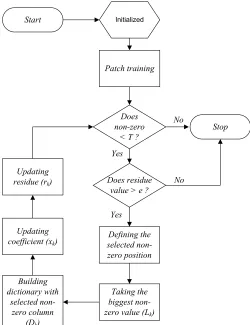
Start Initialized

Patch training

Does non-zero

< T ?

Stop

Does residue value > e ?

Defining the selected non-zero position

Taking the biggest non-zero value (Lk)

Building dictionary with

selected non-zero column

(Dk)

Updating coefficient (xk)

Updating residue (rk)

No

No Yes

Yes

Figure 3: Flowchart of sparse coding process or OMP.

(3)

Start Initialized

Running sparse coding process (OMP

algorithm)

Reducing columns in selected row coefficient by choosing

only non-zero value

Is there any non-zero value at xit index?

Dictionary is not updated Generating i-st signal by

erasing contribution from i-th column in the

dictionary

Finding the residue (Ek)

Updating i-th column and i-th coefficient row of dictionary

by using SVD (Ek)

End

No Yes

Figure 4: Flowchart of K-SVSD algorithm.

III. RESULTS AND DISCUSSION

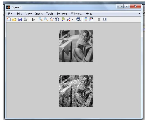
The simulation was running in Intel Pentium B950, 2.1 GHz and with memory of 6.00 GB. For additive noise, we used several level of noise of 10, 15, 20, 25, 50, 75, and 100. We took data 5 times and the value recorded was the average value. The images used in this experiment were the image of Lena, Barbara and boat with a size of 64x64 pixels for each. The example of images using in corpus image training and corrupt image training can be seen in figure 5 and 6 respectively.

Figure 5: Examples of images that were used for corpus image training.

The result of simulation can be seen as follows. Figure 7 shows the result of 30 images trained by the use of EKSVD. It can be seen that the peak signal to noise ratio (PSNR) value of the training before denoising was lower than after. The result proved that EKSVD process was able to reduce the noise. For each experiment, we calculated that the increment of PSNR is about 1.5  3dB for all pictures.

Figure 6: Examples of images that were used for corrupt image training.

Figure 7: PSNR value comparison between before and after denoising by using EKSVD method for 30 images training.

Figure 8: PSNR value comparison between before and after denoising by using EKSVD method for corrupt image training.

Figure 8 shows the result of corrupted image trained by using EKSVD method. It can also be seen that the PSNR value after denoising was greater than before. It proved that the EKSVD method ran effectively to reduce the noise level. We also tried to compare the time consuming process between K-SVD learning dictionary method and EKSVD method for 30 images training as shown in figure 9. Each image was

0 5 10 15 20 25 30 35

σ = 10

σ = 15

σ = 20

σ = 25

σ = 50

σ = 75

σ = 100

P

SN

R

error level

Picture of Lena before denoising

Picture of Lena after denoising

Picture of Barbara before denoising

Picture of Barbara after denoising

Picture of Boat before denoising

Picture of Boat after denoising

0 10 20 30 40

σ = 10

σ = 15

σ = 20

σ = 25

σ = 50

σ = 75

σ = 100

P

SN

R

error level

Picture of Lena before denoising

Picture of Lena after denoising

Picture of Barbara before denoising

Picture of Barbara after denoising

Picture of Boat before denoising

(4)

tested within different noise level and it showed that EKSVD process was faster than K-SVD.

Figure 9: Time comparison between K-SVD learning dictionary and EKSVD for 30 images training.

We also compared the time consuming process between EKSVD method and K-SVD method for corrupted image training as shown in figure 10. Nonetheless, the result also showed that EKSVD process was faster than K-SVD method.

Figure 10: Time comparison between K-SVD learning dictionary and EKSVD for corrupt image training.

For further investigation, we tried to compare the PSNR value for different noises such as Gaussian noise, Salt & Pepper Noise, and Speckle Noise as shown in figure 11. The picture we chose was boat image and the EKSVD method was applied for corrupted image. We found out that the PSNR value was always different for each noise since the kind of noise also influenced its noise distribution.

all the results showed EKSVD method applied for 30 images, as shown in figure 7, could reduce only 6.3% of the noise which was roughly almost similar to K-SVD method [5]. The difference was only 0.05% between EKSVD and K-SVD methods. It means that the EKSVD method was not better than K-SVD one. However, the time consuming for EKSVD was faster than K-SVD as shown in figure 9. The time consuming in total was 40% faster in EKSVD than in KSVD method. In the algorithm design for EKSVD, we focused merely on OMP process combined with MMV. The reading value for atom finding was not per column as in OMP but the learning

process done by taking majority updated values. This led to faster time process although in each row of the dictionary atom was in greater number.

Figure 11: Comparison of PSNR value for corrupt boat image training with EKSVD method and by applying three different kinds of noise.

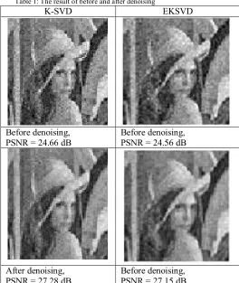
Table 1: The result of before and after denoising

K-SVD EKSVD

Before denoising, PSNR = 24.66 dB

Before denoising, PSNR = 24.56 dB

After denoising,

PSNR = 27.28 dB Before denoising, PSNR = 27.15 dB

For EKSVD process in corrupted image training as shown in figure 8, we found out that this process was slower than K-SVD method. When we tried corrupting image training by using K-SVD method, the number of pixel read by this method was 3249 pixels while for 30 images training was 122880 pixels. In corrupt image training, we applied single image and the pixel reading was overlapping in patch sized of 88 pixels.

0 10 20 30 40 50 60 70 σ = 10 σ = 15 σ = 20 σ = 25 σ = 50 σ = 75 σ = 100 ti m e (s ec o n d ) error level

Picture of Lena with K-SVD

Picture of Lena with EKSVD

Picture of Barbara with K-SVD Picture of Barbara with EKSVD Picture of Boat with K-SVD

Picture of Boat with EKSVD 0 5 10 15 20 25 30 σ = 10 σ = 15 σ = 20 σ = 25 σ = 50 σ = 75 σ = 100 ti m e (s e co n d ) error level

Picture of Lena with K-SVD

Picture of Lena with EKSVD

Picture of Barbara with K-SVD Picture of Barbara with EKSVD Picture of Boat with K-SVD

Picture of Boat with EKSVD 0 10 20 30 40 σ = 10 σ = 15 σ = 20 σ = 25 σ = 50 σ = 75 σ = 100 P SN R error level

Gausian noise before denoising

Gausian noise after denoising

Salt & Pepper noise before denoising

Salt & Pepper noise after denoising

Speckle noise before denoising

(5)

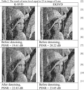
Table 2: The result of noise level equal to 25 in image of Lena

K-SVD EKSVD

Before denoising,

After denoising,

For the comparison of PSNR value in three different kinds of noise, the noise distribution itself had influence in the PSNR value where Gaussian noise could increase the PSNR value as 2.3dB high. In the same time, Salt & Pepper noise could increase the PNSR value up to 2.49 dB and Speckle noise up to 2.56 dB. The average PSNR value increment for each noise was more than 2dB. However, even though PSNR value of the Gaussian noise was lower than any other noises in 10.03 dB, it could still perform better image denoising process than others since its value increased up to 2.3 dB after denoising.

The comparison of image result before and after denoising for both in K-SVD method and EKSVD method can be clearly seen in table 1 and table 2 for noise level of 25.

IV. CONCLUSION

From this experiment, we concluded that the time consuming process for dictionary learning was 40% faster in EKSVD method than in K-SVD method. However, the error reduction was merely quite the same for both methods. We also concluded that the Gaussian noise was the most effective choice for denoising process by seeing its PSNR value. In the future, we will attempt to do experiment by using block sparse K-SVD and will compare its effectiveness with EKSVD that we have now.

REFERENCES

[1] M. Aharon, “Overcomplete Dictionaries for Sparse Representation of

Signals,” Ph.D. dissertation, Dept. of Computer Science, Israel Institute of Technology, 2006.

[2] M. Elad and M. Aharon, “Image Denoising via Sparse and Redundant

Representations Over Learned Dictionaries”, IEEE Transactions on

Image Processing, vol. 15, issue 12, pp. 3736-3745, Dec. 2006.

[3] M. Elad and M. Aharon, “Image Denoising via Learned Dictionaries and

Sparse Representation”, 2006 IEEE Computer Society Conference on

Computer Vision and Pattern Recognition, vol. 1, pp. 895-900. [4] M. Aharon, M. Elad, and A.M. Bruckstein, “On the Uniqueness of

Overcomplete Dictionaries, and a Practical Way to Retrieve them”,

Linear Algebra and Its Applications, vol. 416, issue 1, pp. 48-67, July 2006.

[5] M. Aharon, M. Elad, and A.M. Bruckstein, “K-SVD and its

Non-Negative Variant for Dictionary Design”, Proc. SPIE 5914, Wavelets XI, 591411, Sept. 2005.

[6] M. Aharon and M. Elad, “Sparse and Redundant Modeling of Image

Content Using an Image-Signature-Dictionary”, SIAM J. Imaging Sci., vol. 1, issue 3, pp. 228-247, 2008.

[7] J.A. Tropp and A.C. Gilbert, “Signal Recovery from Random

Measurements via Orthogonal Matching Pursuit”, IEEE Transactions on

Information Theory, vol. 53, issue 12, pp. 4655-4666, Dec. 2007. [8] D.L. Donoho, Y. Tsaig, I. Drori, and J.L. Starck, “Sparse Solution of

Underdetermined Systems of Linear Equations by Stagewise Orthogonal Matching Pursuit”, IEEE Transactions on Information Theory, vol. 58, issue 2, pp. 1094-1121, Feb. 2012.

[9] L. Rebollo-Neira and D. Lowe, “Optimized Orthogonal Matching Pursuit”, IEEE Signal Processing Letters, vol. 9, issue 4, pp. 137-140, April 2002.

[10] M. Gharavi-Alkhansari and T.S. Huang, “A Fast Orthogonal Matching

Pursuit”, Proceedings of the 1998 IEEE International Conference on

Acoustics, Speech and Signal Processing, vol. 3, pp. 1389-1392. [11] S.F. Cotter, B.D. Rao, K. Engan, and K. Kreutz-Delgado, “Sparse

Solutions to Linear Inverse Problems with Multiple Measurement

Vectors”, IEEE Transactions on Signal Processing, vol. 53, issue 7, pp.

2477-2488, July 2005.

[12] Y.C. Eldar, P. Kuppinger, and H. Blocskei, “Block-Sparse Signals:

Uncertainty Relations and Efficient Recovery”, IEEE Transactions on

Signal Processing, vol. 58, issue 6, pp. 3042-3054, June 2010.

[13] Song Shen Liu and M.E. Jernigan, “Texture Analysis and

Discrimination in Additive Noise”, Computer Vision, Graphics, and

Image Processing, vol. 49, issue 1, pp. 52-67, January 1990.

[14] L. Bar, N. Sochen, and N. Kiryati, “Image Deblurring in the Presence of

Salt-and-Pepper Noise”, Scale Space and PDE Methods in Computer Vision, vol. 3459, pp. 107-118, 2005.

[15] K. Chinnasarn, Y. Rangsanseri, and P. Thitimajshima, “Removing Salt

-and-Pepper Noise in Text/Graphic Images”, The 1998 IEEE Asia Pacific

Conference on Circuits and Systems, pp. 459-462.

[16] J.S. Lim and H. Nawab, “Techniques for Speckle Noise Removal”,

Proc. SPIE 0243, Applications of Speckle Phenomena, 35, Dec. 1980.

[17] R. Oktem and N.N. Ponomarenko, “Image Filtering Based on Discrete

Cosine Transform” Telecommunications and Radio Engineering, vol.

66, pp. 1685-1701, 2007.

[18] G. Strang, “The Discrete Cosine Transform”, SIAM Rev., vol. 41, issue

1, pp. 135-147, 1999.

[19] N. Ahmed, T. Natarajan, and K.R. Rao, “Discrete Cosine Transform”,

IEEE Transactions on Computers, vol. C-23, issue 1, pp. 90-93, January 1974.

[20] Z.M. Hafed and M.D. Levine, “Face Recognition Using the Discrete

Cosine Transform”, International Journal of Computer Vision, vol. 43, issue 3, pp. 167-188, 2001.

[21] Jie Yang, A. Bouzerdoum, and Son Lam Phung, “A New Approach to

Sparse Image Representation Using MMV and K-SVD”, Advanced Concepts for Intelligent Vision Systems, vol. 5807, pp. 200-209, 2009.