IPPI DOI: 10.22063/poj.2018.2318.1125
Development of a rheological model for polymeric
fluids based on FENE model
Hossein Ebrahimi
1, Ahmad Ramazani S.A.
1*, Seyed Mohammad Davachi
2,31Polymer Group, Department of Chemical and Petroleum Engineering, Sharif University of Technology, Tehran, Iran 2Soft Tissue Engineering Research Center, Tissue Engineering and Regenerative Medicine Institute, Central Tehran
Branch, Islamic Azad University, Tehran, Iran
3Department of Chemical and Polymer Engineering, Faculty of Engineering, Central Tehran Branch, Islamic Azad University, Tehran, Iran
Received: 15 October 2018, Accepted: 23 November 2018
ABSTRACT
R
heological models for polymer solutions and melts based on the finitely extensible non-linear elastic (FENE) dumbbell theory are reviewed in this study. The FENE-P model that is a well-known Peterlin approximation of the FENE model, indicates noticeable deviation from original FENE predictions and also experimental results, especially in the transient flow. In addition, both FENE and FENE-P models have some shortcomings from the point of view of theory. To overcome these shortcomings, a new approximation of the FENE spring force has been established. It has been used to develop a modified constitutive rheological model for polymeric fluids. In the procedure of modeling, the effect of non-affine deformation is introduced into the new model. Comparison between the model predictions and experimental data presented in the literature for transient and steady shear flow of polystyrene indicates that this modified model can predict the rheological behavior of polymeric fluids with a great accuracy. The newly developed modified model could predict different slopes that can cover the behavior of most of the polymeric fluids. Polyolefins J (2019) 6: 95-106Keywords: Rheological modeling, spring force approximation, FENE model, FENE-P model, FENE-M2 model, FENE modification.
* Corresponding Author - E-mail: [email protected]
INTRODUCTION
Finitely extensible non-linear elastic dumbbell is a molecular concept of a polymer chain that has been used to describe non-Newtonian rheological effects in polymer solutions and melts [1–7]. FENE model has a vital role in explaining complicated and more realistic physical phenomena of molecular behaviors [8–10]. FENE model predicts the shear-thinning viscosity, first normal stress coefficient and a plateau in the extensional viscosity at high extension rates [11, 12]. This model is reformed to the developed models or systems, such as
FENE-P [13], FENE-L, FENE-LS [14, 15], FENE-S, D, QE, QE- PLA [16, 17], FENE-PM [18], FENE-M, FENE-MR, FENE-LSM, and FENE-LSMR [19]. A complete review of the FENE and its modifications has been done by Venkataramani et al. [3] and Hyon et al. [16]. Except for some simple flows, the FENE model is very challenging and time-consuming to handle and a closure approximation such as the FENE-P model especially when dealing with complex flows is needed [20, 21]. The FENE-P model indicates a noticeable deviation from the original FENE predictions and also experimental results especially in
the transient flow [14, 15, 19, 20, 22, 23]. In addition, the original FENE and existing closure models have some shortcomings from theoretical aspects.
In this work at first, classical rheological modeling based on FENE theory is reviewed, and some shortcomings of FENE and FENE-P models are investigated. Then, a new approximation of FENE spring force and a rheological constitutive model based on the new approximation are developed. The model is solved in transient and steady shear flows. The effects of the model parameters on the model predictions are investigated. Finally, experimental data that are taken from the literature are compared with model predictions.
THEORETICAL
Review of classical rheological modeling based on FENE theory
The simplest mechanical models for flexible polymer molecules are the elastic dumbbell models, where two beads, each of mass m, are joined by a non-bendable spring [24]. The tension in the spring is denoted by FC. The location of the beads is given by the position vector rv (ν=1, 2), with respect to an arbitrary origin of coordinates and the velocity of the bead is r=d dtr / of the same origin. The mass center rc of macromolecule is rc=1/2(r1+r2), and its velocity is rc. The connector vector or end-to-end vector
Q=r2-r1 describes the overall orientation and internal configuration of the polymer molecules. Each bead is presumed to experience a Stokes’ law drag force. According to Stokes' law the drag force is assumed to be proportional to the relative velocity between solvent and bead, with a proportionality constant z called the friction coefficient [24, 25]. The beads represent molecular segments having several monomers, and the spring describes the entropic effects in which the end-to-end vector of the polymer is the subject [22]. The flow field of the polymer solution is taken to be homogeneous, then the mass average velocity of the solution can be written as v = v0+ [k.r] where v0 is a vector independent of position and kt=Ñv is the velocity gradient tensor which is independent of the position vector r in the fluid, and its trace has zero value due to the assumption of fluid incompressibility. The Fokker-Planck equation governing the evolution of the configurational distribution function Y(Q,t) is [24, 26]:
) 2 2
] . .{[
( y
z y z y
y B c
Q T k Q
t Q ∂ − F
∂ − ∂
∂ − = ∂
∂ k (1)
Where kB is the Boltzmann constant, and T is the temperature in Kelvin. In equation (1) the first term on the right-hand side accounts for the hydrodynamic drag forces on the beads due to the dumbbell's movement through the solvent. The second term describes the Brownian motion force on the beads because of thermal fluctuations in the solvent, and the last one accounts for the forces transmitted through the connecting spring. The diffusion coefficient kBT/2z is assumed to be constant. For a function B(Q) of the connector vector, the time-dependent configuration space average is given by the following equation:
Q Q Q) ( , ) 3
( t d
B
B =∫ y (2)
Therefore, from the Fokker-Planck equation [24, 26], the equation of motion for the second moments of the distribution function for the end-to-end vector can be obtained as follows:
c B
t k T t
dd QQ =k.QQ + QQ.k +4z d−z4 QF (3) Where QQ is the second moment of configuration tensor and d is the unit tensor. The polymer contribution to the stress tensor, from the Kramer’s expression, can be obtained as [24]:
d
sp =−nQFC +nkBT (4)
Where n is the number of macromolecules in the unit volume. To complete the model presentation, it is enough to introduce the spring force into equations (3) and (4). The simplest form of spring force is linear Hookean, that denotes by FC(Hookean) and takes the
following manner [24, 27]:
( )
C Hookean
F =HQ (5)
To describe non-Newtonian rheological effects in polymer solutions, the finitely extensible non-linear elastic (FENE) spring force was introduced by Warner et al. [29]:
( )
C FENE
2 2
0
1 /
H Q Q
= −
F Q (6)
Where Q0 is the maximum extension of polymer chains. By using the spring force equation (6), there is no closed constitutive equation for the polymeric stress tensor, and no simple analytical solutions are possible [24]. An analytically more tractable dumbbell model which leads to a final constitutive equation can be attained by substituting the configuration-dependent non-linear factor in the FENE spring force by a self-consistently averaged term [24]:
( )
C FENE P
2 2 0
1 /
H Q Q − =
− < >
F Q (7)
This pre-averaging spring force is known as the Peterlin approximation and the resulting model as the FENE-P model. In the FENE and FENE-P models,
lH=z/4H and b=HQ02/K
BT called relaxation time and extensibility parameter, respectively. Although most widely used non-linear kinetic models are FENE and its closure approximations, there are some shortcomings in the FENE and FENE-P models: i. Based on Larson [30], when a chain end extends to increase the end-to-end distance Q, the needed force to overcome the entropic "spring" force of the chain is as follows:
Q F 2K Tb2
B
C = (8)
where,
2 2
Q
2
3
=
b
(9)
By replacing the β from equation 9 to 8, the entropic force will be obtained as follows:
C B
2 3K T
Q
=
F Q (10)
On the other hand, at equilibrium (steady state with
k
=0), d 0dt QQ = , therefore, based on equation 3, the
can be easily obtained as: d
T kB q e
C =
F
Q
(11)
It is known that, at equilibrium, 2
eq
Q =tr QQ ,
accordingly, Q2 will be generated as follows:
2 3K TB Q
H
= (12)
Finally, from equations 10 - 12:
d
)
/ (kBT H q
e = Q
Q
(13)
According to Herrchen and Öttinger (Herrchen and Öttinger 1997), the equilibrium state for the second moment of the FENE is QQ eq =(kBT/H)[b (/b+5)]d and those of for the FENE-P model is
d ] ) 3 (/ [ ) /
( +
= kBT H b b q
e
Q
Q . Therefore, the equation
13 for the FENE and FENE-P model will be satisfied just for b→∞. The obtained results are in accordance
with the previous reports by Stephanou et al. [31]. In the real condition, the spring can be pulled to fully extent state, this means the polymer chain is in the fully stretched-out conformation. In this condition, FENE and FENE-P models calculate infinite value for spring force, in contrary with real condition.
ii. In the FENE and FENE-P models, the maximum extension of the polymer chain is Q0, then at 2 2
0
Q =Q
the spring force will be infinite based on mathematical equations because Fc will be infinite, but indeed, the spring force should have a finite value in the physical or real conditions.
iv. The original FENE and FENE-P models predict only a constant value for the slope of the linear or power-law region in steady shear flow. In addition, the prediction of the models for second normal stress coefficient y2 is zero, and then they could not predict any value for y2/y1.
To overcome the above shortcomings of the FENE and FENE-P models, a more convenient approximation of FENE spring force has been developed. Then a rheological model based on modified spring force has been presented. In addition, the effects of the non-affine deformation have been introduced into the modified model.
MODEL FORMATION
Spring force
As mentioned before, to overcome shortcomings of the FENE and FENE-P models, a new spring force approximation was introduced, which henceforth denotes FC(FENE-M2), as follows:
Q F 2 q e 2 0 2 2 ) 2 ( 1 Q Q q e Q Q H M FENE C e + > < − − =
− (14)
Where ε is a phenomenological parameter. On the contrary with the FENE and FENE-P models, in this modified introduced spring force the second moment of the end-to-end vector of polymer chain at equilibrium condition is <QQ>eq=(kBT/H)d. In addition, the spring force would have a finite value at 2 2
0
Q =Q .
In the new form of spring force presentation, it has been assumed that the polymer chain can be extended a few more than Q0. At Q2=Q02 the polymer chain is under the fully stretched-out conformation. If the stretching continues, the bonds of the chain will start to extend. The maximum value of the chain extension is indicated by 2
q e 2 0 2
max Q Q
Q = +e or 2 3e
max=b+
Q in
dimensionless form. Therefore, the acceptable values for e are e>-b/3.
Constitutive equation presentation
The following dimensionless forms of variables and parameters have been introduced to simplify the model presentation:
k T k n t t H T K Q H B p p H B l s s
l = =
= = * * * 2 / 1 * ; ; ; ) / ( k
Q (15)
Replacing equation (14) in (3) results in:
* * * * * * * * * * *
* 3 3
3 .
.
Q Q Q Q Q Q Q Q r t b b t d d t − + + + − + + = e e d k k (16)
The contribution of polymer in the stress tensor can be demonstrated as follows in case of replacing equation (14) in (4):
d e e s + − + + + − * * * * * 3 3
3 QQ
Q Q r t b b
p (17)
Where tr represents trace. To simplify more in equations (18) and (19), M*= Q Q* * is assigned. Also,
the transpose of the velocity gradient tensor k* can be written as follows:
)
(
2
/
1 γ w
k∗=
l
H − (18)Where γ is the rate of strain tensor and is the vorticity
tensor. Now equations (16) and (17) are rewritten in a new form as follows:
* * * * * * * * 3 3 3 ) . . ( 2 1 ) . . ( 2 1 M M M M M M M tr b b t d d − + + + − + − − + = e e d w w γ γ (19) d e e s + − + + + − = * * * 3 3 3 M M r t b b
p (20)
The developed model is called FENE-M2 approximation on FENE spring force.
Introducing the non-affine deformation
In the study of dumbbell kinetic theory, it has been assumed that the two beads of the dumbbell move through the solvent without disturbing the velocity field [33, 34]. Therefore, the velocity of fluid in each bead is as same as the velocity of fluid (that is
n=n0+[k.r]). An alternative procedure to introduce the effect of the flow perturbation at bead n resulting from the motion of the other beads is to replace the fluid velocity at bead by the following equation:
] ) -.( [ 2 1 ] .
[ v c
0 r r r
v
vv = + k v − z γ (21)
If this alternative procedure is introduced to the FENE-M2 model, the time evolution equation (21) will be as follows:
* * * * * * * * 3 3 3 ) . . ( 2 1 ) . . ( 2 1 M M M M M M M r t b b t d d − + + + − + − − + = e e d w w γ γ (22)
By this modification, the value of the second normal stress coefficient will be non-zero and Y2/Y1=-1/2z [24, 35, 36]. Constitutive equations, which have the GS derivative, show unreal oscillations in the start-up shear flow material functions curve [38, 39]. This problem will be investigated in Section 4.2.
RESULTS AND DISCUSSION
Equation (22) represents a system of ordinary differential equations that is solved numerically both for transition and steady shear flows. The initial condition is the equilibrium state Meq*=d and the model parameters are b, e and z. In simple shear flow, the velocity field is given by vx=γyxy, vy =0
and vz=0 where γyx is the velocity gradient and can
be a function of time. The absolute value of γyx is
called the shear rate and denoted by γ. Thus, the rate
of strain tensor and the vorticity tensor are as follows:
− = = 0 0 0 0 0 1 0 1 0 ) ( ) ( , 0 0 0 0 0 1 0 1 0 ) ( )
(t γ t w t γ t
γ (23)
The stress tensor has the following form with sxy=syx.
= 1 0 0 0 0 y y x y y x x x s s s s
s (24)
For steady shear flow (sometimes called a viscometric flow) the shear rate does not depend on the time, it is presumed that the shear rate has been constant for so long that all the stresses in the fluid are time-independent [24, 40]. The dimensionless shear viscosity η is defined analogously to the viscosity of Newtonian fluids:
γ l s l h γ s H B y x p H B y x p T k n T k n , *
, or )
( =− ∗ =−
∗ γ
h (25)
Likewise, the dimensionless first and second normal stress coefficients *
1
y and * 2
y can be defined as follows,
Where γ*=lHγ is the dimensionless shear rate and
* j i
s are the components of the extra stress tensor given by equation (20):
2 y , , 2 1 2 * y , * x , *
1( ) or ( ) (l γ)
s s l γ y γ s s H B y p x x p H B y p x p T k n T k n − − = − − = ∗ γ y (26) 2 Z , , 2 2 2 * z , * y , *
2( ) or ( ) (l γ)
s s l γ y γ s s H B Z p Y Y p H B z p y p T k n T k n − − = − − = ∗ γ y (27)
For each transient shear flow as in steady shear flow the relevant material functions are the viscosity η±, and
the first and second normal stress coefficients Y1± and Y2±. The plus and minus signs are used for start-up
and relaxation material functions, respectively. These are given in dimensionless form by equation (28):
2 * * z , * y , * 2 2 * * y , * , * 1 * , , ( ) , ( ) )
( sγ s γ s s γ s
=− pxy ± =− pxx− p y ± =− p y− p z
∗ ±
∗ γ y γ y γ
h
(28)
Therefore, in transient flow the curves of η, Y1 and Y2
versus time describe the time-dependent rheological behavior of polymeric materials. In the following subsections, the effects of the influencing parameters on the model prediction will be investigated.
Effects of the slip parameter on the model predictions
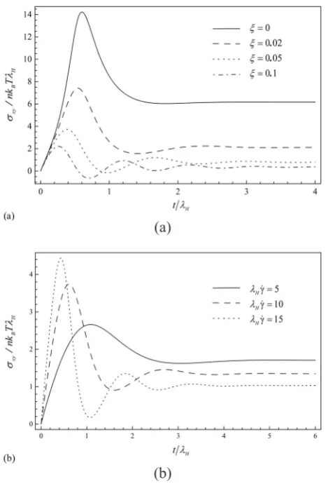
As it is mentioned, introducing x into the model causes an oscillation in the material functions curve versus time in the start-up shear flow. Figure 1(a) indicates that at the given shear rate for small values of x, there is no oscillation in the curve of shear stress versus time. The oscillations in the curve are appeared as x
is increased.
about z <15/([b+e)lHγ] [43–45].
Figures 2(a) and 2(b) depict the influence of slip parameter x on the transient material functions, h±
and Y1± , respectively. The results indicate that the
size of overshoot and steady state plateau values are decreased via increasing x. In Figure 3 the effect of the slip parameter on the shear rate dependent viscosity is presented. As it is seen for selected model parameters, increasing x from zero to 0.004 changes the slope of curve from -0.66 to -0.98.
Effects of the eparameter on the model predictions
The role of e which is a new parameter introduced
into the FENE-M2 model, is investigated. To clarify the effect of e on the model predictions, a comparison
between FENE, FENE-P and FENE-M2 model`s predictions in transient shear flows is done. As mentioned before, to choose a value for e, one should
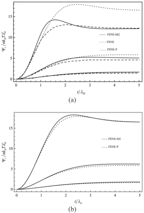
notice that the acceptable values for e are e>-b/3. Figure
4(a) exhibits the evolution of the time in the first normal stress difference during start-up of shear flow for three models. The results indicated the FENE-P model is over prediction than the FENE model, especially at higher shear rates. The more shear rate increases, the more value of over predictions can be seen. It could be seen that the FENE-M2 predictions are so close to those of the FENE model for chosen parameters. It is possible to make the FENE-M2 predictions closer into the FENE or FENE-P by selecting different values of e. Figure 4(b) shows the FENE-M2 and FENE-P
predictions for the first normal stress difference with respect to chosen model parameters which are nearly coincident when .
The effect of e parameter on the transient material functions, h± and Y
1±, is survived in Figures 5(a) and
5(b), respectively. An increasing in e value grows the steady value of material functions. Besides, for both material functions, the overshoot occurs at a later time with increasing e.
Figure 6(a) and (b) represents the effect of e on
Figure 1. Oscillations in the curve of shear stress vs. time in the start-up shear flow with model parameters b=50 and
e=0:(a) Dimensionless shear rate has fixed value lHγ=15
and slip parameter has different values. (b) Slip parameter has fixed value x=0.04 and dimensionless shear rate has different values.
Figure 2. Effect of the slip parameter on the stress growth and relaxation of material functions with the dimensionless shear rate lHγ=5 and the model parameters b=50 and e=0:
(a) viscosity and (b) first normal stress coefficient.
(a)
(b)
(a)
the steady material functions, η and Y1, respectively. As it can be seen, increasing of e would increase the
length of the plateau with no change in the slope of the curve. In the other hand, the “power law exponent” is independent of e values.
Effects of the extensibility parameter on the model predictions
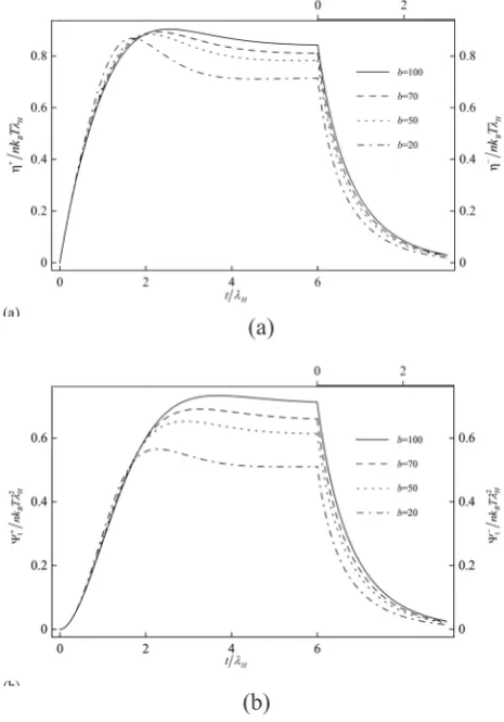
The transient viscosity and the first normal stress difference coefficient at different values of extensibility parameter are presented in Figures 7(a) and 7(b). As it is seen, for both material functions, η± and Y
1±, the steady values grow with increasing b. In addition, the overshoot occurs at a later time with increasing b.
Figures 8(a) and 8(b) display the influence of extensibility parameter on the steady viscosity and the first normal stress difference, respectively. Similarly, to the e effect, for both material functions increasing of b would increase the length of plateau. Also, the exponent of the power law is again independent of the extensibility parameter b.
Figure 3. Effect of the slip parameter on the steady viscosity with the model parameters b=50 and e=6.
Figure 4. Comparison between the FENE, FENE-P and FENE-M2 models in the prediction of the first normal stress difference in the start-up of shear flow. The model parameters are b=50 and x=0 and the dimensionless shear rates are lHγ=1,2 and 4 (from down to top): (a) With e =-3.5 the results of FENE-M2 and FENE models are close them (b) With e=-11.2 the results of FENE-M2 and FENE-P models nearly are coincident. Data for FENE model reproduced from van Heel et al. [32].
Figure 5. Effect of e parameter on the stress growth and relaxation of material functions with dimensionless shear rate lHγ =4 and model parameters b=20 and x=0: (a)
viscosity and (b) first normal stress coefficient.
(a)
(b)
(a)
Effects of the shear rate on the model predictions
Figures 9(a) and 9(b) show the effect of the shear rate on the transient material functions, h± and Y
1±,
respectively.
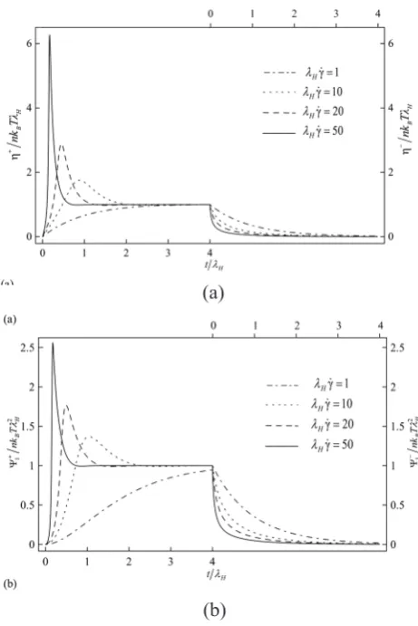
The results indicate that there is no overshoot or
related phenomenon for low shear rates. The viscosity and the first normal stress difference show an overshoot when the shear rate increases to its larger values. The size of this overshoot increases by increasing the shear rate while the time corresponding to its maximum
Figure 6. Effect of e parameter on the steady material functions with model parameters b=20 and x=0: (a) viscosity and (b) first normal stress coefficient.
Figure 7. Effect of the extensibility parameter b on the material functions with dimensionless shear rate lHγ=4
and model parameters e=6 and x=0: (a) viscosity and (b) first normal stress coefficient.
Figure 8. Effect of the extensibility parameter b on the steady material functions with model parameters e=6 and
x=0: (a) viscosity and (b) first normal stress coefficient.
(a)
(b)
(a) (b)
(a)
value decreases as the shear rate increases [41, 46]. Besides, relaxation curves show that both material functions relax monotonically to zero in low shear rate and then it relaxes more rapidly as the shear rate increases.
Comparison with experimental data
The comparison between the model prediction and experimental data (taken from Schweizer et al. [47]) in the start-up shear flow is presented in Figure 10 for polystyrene melt at 175°C and three shear rates 0.1, 1 and 3 s-1. The results indicate that the experimental data are in good agreement with model predictions.
Figure 11 compares the model prediction in start-up shear flow for the first normal stress difference, N1, and the experimental data taken from Schweizer et al. [47]. The presented results show that model predictions are in qualitative and quantitative agreement with experimental results.
Figure 12 presents the model predictions with counterpart experimental data taken from Laun study for LDPE melt at 150°C in the steady shear flow for the viscosity and the first normal stress difference [48].
Figure 9. Effect of the shear rate on the transient material functions. Model parameters are b=50, e=0 and x=0: (a) viscosity and (b) first normal stress coefficient.
Figure 10. Comparison between the model prediction and experimental date in the start-up viscosity shear flow. Model parameters are b=20, e=4 and x=0.03. Data are taken from Schweizer et al. [47].
Figure 11. Comparison between the model prediction and experimental date for the first normal stress difference in start-up shear flow with γ=10s-1. Model parameters are
b=20, e=4 and x=0.03. Data are taken from Schweizer et al. [47].
Figure 12. Comparison between the model prediction and experimental data for the viscosity and the first normal stress difference in the steady shear flow. Model parameters are b=18, e=0 and x=0. Data are taken from Schweizer et al. [47].
(a)
As it is seen, the model predictions are in excellent agreement with experimental data.
CONCLUSION
In the review of the FENE and FENE-P models, some shortcomings of these models are highlighted. Prediction results in the transient flow indicate a significant difference between model predictions by original FENE and its approximation FENE-P. A new closure approximation for spring force has been developed and used to develop a modified FENE based (FENE-M2) model. The presented results indicate that this closure approximation should be closer to the original FENE than Peterlin approximation. In the procedure of modeling, the effect of non-affine deformation is studied and a parameter called slip parameter is introduced into the model to improve model prediction behavior. Where the FENE and FENE-P models predict only a constant slope for material functions in steady shear flow curves, the newly developed modified model could predict different slopes that can cover the behavior of most polymeric fluids. Comparison of the model predictions with experimental data shows the FENE-M2 model can predict the behavior of polymeric fluids in the steady and transient shear flow correctly.
REFERENCES
1. Ait-Kadi A, Ramazani A, Grmela M, Zhou C (1999) “Volume preserving” rheological models for polymer melts and solutions using the GENERIC formalism. J Rheol 43: 51–72 2. Eslami H, Ramazani S. A. A, Khonakdar HA (2004)
Predictions of Some Internal Microstructural Models for Polymer Melts and Solutions in Shear and Elongational Flows. Macromol Theory Simul 13: 655–664
3. Venkataramani V, Sureshkumar R, Khomami B (2008) Coarse-grained modeling of macromolecular solutions using a configuration-based approach. J Rheol 52: 1143–1177 4. Zhiyu M, Wei C, Changyu S (2008) Numerical
study of dilute polymer solutions using FENE bead-spring chain model. Polym-Plast Technol Eng 47: 630–634
5. Ommati M, Ahmadi IF, Davachi SM, Motahari S (2011) Erosion rate of random short carbon fibre/phenolic resin composites: Modelling and experimental approach. Iran Polym J 20: 943–954 6. Mousavi SM, Ramazani A, Najafi I, Davachi
SM (2012) Effect of ultrasonic irradiation on rheological properties of asphaltenic crude oils. Pet Sci 9: 82–88
7. Larson RG, Desai PS (2015) Modeling the rheology of polymer melts and solutions. Annu Rev Fluid Mech 47: 47–65
8. Warner Jr HR (1972) Kinetic theory and rheology of dilute suspensions of finitely extendible dumbbells. Ind Eng Chem Fundam 11: 379–387 9. Pishdad A, Kaffashi B, Davachi SM (2012)
Investigation of Dispersion, Interaction and Superstructure Formation in PTMEG/MWCNT Nanocomposites. Sci Technol 25: 289–300 10. Sahraeian R, Davachi SM, Heidari BS (2019)
The effect of nanoperlite and its silane treatment on thermal properties and degradation of polypropylene/nanoperlite nanocomposite films. Compos Part B Eng 162:103–111
11. Herrchen M, Öttinger HC (1997) A detailed comparison of various FENE dumbbell models. J Non-Newton Fluid Mech 68: 17–42
12. Wiest JM, Tanner RI (1989) Rheology of bead-nonLinear spring chain macromolecules. J Rheol 33: 281–316
13. Wedgewood LE, Bird RB (1988) From molecular models to the solution of flow problems. Ind Eng Chem Res 27: 1313–1320
14. Lielens G, Halin P, Jaumain I, et al (1998) New closure approximations for the kinetic theory of finitely extensible dumbbells. J Non-Newton Fluid Mech 76: 249–279
15. Lielens G, Keunings R, Legat V (1999) The FENE-L and FENE-LS closure approximations to the kinetic theory of finitely extensible dumbbells. J Non-Newton Fluid Mech 87: 179–196
16. Hyon Y, Carrillo JA, Du Q, Liu C (2008) A maximum entropy principle based closure method for macro-micro models of polymeric materials. Kinet Relat Models 1: 171–184
17. Ahmad A, Vincenzi D (2016) Polymer stretching in the inertial range of turbulence. Phys Rev E 93: 052605
Mech 40: 119–139
19. Zhou Q, Akhavan R (2004) Cost-effective multi-mode FENE bead-spring multi-models for dilute polymer solutions. J Non-Newton Fluid Mech 116: 269–300
20. Lhuillier D (2001) A possible alternative to the FENE dumbbell model of dilute polymer solutions. J Non-Newton Fluid Mech 97: 87–96 21. Vincenzi D, Perlekar P, Biferale L, Toschi F
(2015) Impact of the Peterlin approximation on polymer dynamics in turbulent flows. Phys Rev E 92: 053004
22. Herrchen M, Öttinger HC (1997) A detailed comparison of various FENE dumbbell models. J Non-Newton Fluid Mech 68: 17–42
23. Keunings R (1997) On the Peterlin approximation for finitely extensible dumbbells. J Non-Newton Fluid Mech 68: 85–100
24. Bird RB, Curtiss CF, Armstrong RC, Hassager O (1987) Dynamics of polymeric liquids, Vol 2: Kinetic theory, Wiley
25. Schneggenburger C, Kröger M, Hess S (1996) An extended FENE dumbbell theory for concentration dependent shear-induced anisotropy in dilute polymer solutions. J Non-Newton Fluid Mech 62: 235–251
26. Ammar A (2016) Effect of the inverse Langevin approximation on the solution of the Fokker– Planck equation of non-linear dilute polymer. J Non-Newton Fluid Mech 231: 1–5
27. Renardy M (2013) On the eigenfunctions for Hookean and FENE dumbbell models. J Rheol 1978-Present 57: 1311–1324
28. Heidari BS, Cheraghchi V-S, Motahari S, et al (2018) Optimized mercapto-modified resorcinol formaldehyde xerogel for adsorption of lead and copper ions from aqueous solutions. J Sol-Gel Sci Technol 88: 236–248
29. Warner Jr HR (1972) Kinetic theory and rheology of dilute suspensions of finitely extendible dumbbells. Ind Eng Chem Fundam 11: 379–387 30. Larson RG (1999) The structure and rheology of
complex fluids, 1st Ed, Oxford University Press, New York, p.114
31. Stephanou PS, Baig C, Mavrantzas VG (2009) A generalized differential constitutive equation for polymer melts based on principles of nonequilibrium thermodynamics. J Rheol 53: 309–337
32. Van Heel APG, Hulsen MA, Van den Brule B
(1998) On the selection of parameters in the FENE-P model. J Non-Newton Fluid Mech 75: 253–271
33. Heidari BS, Davachi SM, Moghaddam AH, et al (2018) Optimization simulated injection molding process for ultrahigh molecular weight polyethylene nanocomposite hip liner using response surface methodology and simulation of mechanical behavior. J Mech Behav Biomed Mater 81: 95–105
34. Heidari BS, Oliaei E, Shayesteh H, et al (2017) Simulation of mechanical behavior and optimization of simulated injection molding process for PLA based antibacterial composite and nanocomposite bone screws using central composite design. J Mech Behav Biomed Mater 65: 160–176
35. Gordon RJ, Schowalter WR (1972) Anisotropic fluid theory: a different approach to the dumbbell theory of dilute polymer solutions. Trans Soc Rheol 16: 79–97
36. Öttinger HC (2005) Beyond equilibrium thermodynamics. John Wiley & Sons 37. Huang S, Lu C, Fan Y (2006) Time-dependent
viscoelastic behavior of an LDPE melt. Acta Mech Sin 22: 199–206
38. Bhat PP, Pasquali M, Basaran OA (2009) Beads-on-string formation during filament pinch-off: Dynamics with the PTT model for non-affine motion. J Non-Newton Fluid Mech 159: 64–71 39. Larson RG (2013) Constitutive equations for
polymer melts and solutions. In: Butterworths series in chemical engineering, Elsevier Science 40. Binetruy C, Chinesta F, Keunings R (2015) Multi-scale Modeling and Simulation of Polymer Flow. In: Flows in polymers, reinforced polymers and composites, Springer International Publishing, pp 1–42
41. Parsa P, Paydayesh A, Davachi SM (2019) Investigating the effect of tetracycline addition on nanocomposite hydrogels based on polyvinyl alcohol and chitosan nanoparticles for specific medical applications. Int J Biol Macromol 121: 1061–1069
42. Davachi SM, Shekarabi AS (2018) Preparation and characterization of antibacterial, eco-friendly edible nanocomposite films containing Salvia macrosiphon and nanoclay. Int J Biol Macromol 113: 66–72
O (1987) Dynamics of polymeric liquids, Vol. 2: Kinetic theory. Wiley
44. Cook LP, Rossi LF (2004) Slippage and migration in models of dilute wormlike micellar solutions and polymeric fluids. J Non-Newton Fluid Mech 116: 347–369
45. Öttinger HC (2005) Beyond equilibrium thermodynamics. John Wiley & Sons 46. Balali S, Davachi SM, Sahraeian R, et al (2018)
Preparation and characterization of composite blends based on polylactic acid/polycaprolactone and silk. Biomacromolecules 19: 4358–4369 47. Schweizer T, van Meerveld J, Ottinger HC (2004)
Nonlinear shear rheology of polystyrene melt with narrow molecular weight distribution-Experiment and theory. J Rheol 48:1345–1364