Volume 8 - Article 11 | Pages 305–358

of peer-reviewed research and commentary in the population sciences published by the Max Planck Institute for Demographic Research Konrad-Zuse Str. 1, D-18057 Rostock · GERMANY www.demographic-research.org

DEMOGRAPHIC RESEARCH

VOLUME 8, ARTICLE 11, PAGES 305-358

PUBLISHED 17 JUNE 2003

www.demographic-research.org/Volumes/Vol8/11/

DOI: 10.4054/DemRes.2003.8.11

Research Article

Gini coefficient as a life table function:

computation from discrete data,

decomposition of differences and

empirical examples

Vladimir M. Shkolnikov

Evgueni E. Andreev

Alexander Z. Begun

1 Introduction 306

2 Definitions and properties 308

2.1 The Lorenz curve 308

2.2 Application to the distribution of length of life 308

2.3 Gini coefficient 310

2.4 Basic properties of inequality measures 313

3 Empirical trends in Gini coefficient and other measures of inequality and judgements about direction of changes in inequality

314

4 Computation of Gini coefficient from complete and abridged life tables

318

5 Decomposition of a difference between two values of Gini coefficient

324

5.1 Age 324

5.2 Age and cause of death 328

5.3 Age, mortality and population structure 332

6 Variations in life expectancy and Gini coefficient in time and across countries

338

7 Conclusion 343

8 Acknowledgements 345

Notes 346

References 347

Appendix 1 352

Appendix 2 353

Appendix 3 354

Research article

Gini coefficient as a life table function:

computation from discrete data, decomposition of

differences and empirical examples

Vladimir M. Shkolnikov 1

Evgueni E. Andreev 2

Alexander Z. Begun 3

Abstract

This paper presents a toolkit for measuring and analyzing inter-individual inequality in length of life by Gini coefficient. Gini coefficient and four other inequality measures are defined on the length-of-life distribution. Properties of these measures and their empirical testing on mortality data suggest a possibility for different judgements about the direction of changes in the degree of inequality by using different measures. A new computational procedure for the estimation of Gini coefficient from life tables is developed and tested on about four hundred real life tables. The estimates of Gini coefficient are precise enough even for abridged life tables with the final age group of 85+. New formulae have been developed for the decomposition of differences between Gini coefficients by age and cause of death. A new method for decomposition of age-components into effects of mortality and composition of population by group is developed. Temporal changes in the effects of elimination of causes of death on Gini coefficient are analyzed. Numerous empirical examples show: Lorenz curves for Sweden, Russia and Bangladesh in 1995, proportional changes in Gini coefficient and four other measures of inequality for the USA in 1950-1995 and for Russia in 1959-2000. Further shown are errors of estimates of Gini coefficient when computed from various types of mortality data of France, Japan, Sweden and the USA in 1900-95,

1 _{Max Planck Institute for Demographic Research. Correspondence to: Max Planck Institute for}

Demographic Research, Konrad-Zuse-Str., 1, D-18057 Rostock, Germany. Tel: (49 381) 2081 147; Fax: (49 381) 2081 447. E-mail: [email protected]

decompositions of the USA-UK difference in life expectancies and Gini coefficients by age and cause of death in 1997. As well, effects of elimination of major causes of death in the UK in 1951-96 on Gini coefficient, age-specific effects of mortality and educational composition of the Russian population on changes in life expectancy and Gini coefficient between 1979 and 1989. Illustrated as well are variations in life expectancy and Gini coefficient across 32 countries in 1996-1999 and associated changes in life expectancy and Gini coefficient in Japan, Russia, Spain, the USA, and the UK in 1950-1999. Variations in Gini coefficient, with time and across countries, are driven by historical compression of mortality, but also by varying health and social patterns.

1. Introduction

At present, the average level of length of life is high in many countries and it is interesting to study to what extent this advantage is equally accessible to all people. This is why measures of variability in respect to length of life attract growing attention (Anand et al., 2001).

Gini coefficient is the most common statistical index of diversity or inequality in social sciences (Kendall and Stuart, 1969, Allison, 1978). It is widely used in econometrics as a standard measure of inter-individual or inter-household inequality in income and wealth (Atkinson, 1970 and 1980, Sen, 1973, Anand, 1983). Gini coefficient can also be used as a measure of inequality in length of life (or as a degree of inter-individual variability in age at death).

In a number of studies, Gini coefficient has been applied to mortality schedules. In some studies, Gini coefficient has been used to measure variability in levels of mortality among socio-economic groups (Leclerc et al., 1990). However, in most studies it expressed inter-individual variability in age at death (Le Grand, 1987, 1989, Illsey and Le Grand, 1987, Silber, 1988, 1992, Llorka et al., 1998).

Illsey and Le Grand (1987) computed Gini coefficient from distributions of deaths by age in real populations. Other researchers linked Gini coefficient and other measures of inter-individual inequality in age at death with the life table (Hanada, 1983, Silber, 1992, Wilmoth and Horiuchi, 1999, Anand and Nanthikesan, 2000, Anand et al., 2001).

Hicks proposed to use Gini coefficient to adjust average life expectancy for variability in order to construct the inequality-adjusted human development index (Hicks, 1997).

Gini coefficient has also been considered among other indices of inequality, as a measure of the rectangularization of survival curves in human populations (Wilmoth and Horiuchi, 1999). This approach is closely linked to the broader concept of studying historical evolution of human mortality, mortality compression, and limits of the human life span (Fries, 1980, Myers and Manton, 1984, Kannisto et al., 1994, Wilmoth and Lundström, 1996, Lynch and Brown, 2001).

The purpose of the present study is mostly a practical one. It is aimed at developing a toolkit for operating with Gini coefficient, similar to the one used for analyzing average life expectancy.

The first section of the study briefly presents a theoretical framework for measuring a degree of inter-individual inequality in length of life. It provides definitions and describes the basic properties of Gini coefficient, as well as four other measures of inequality in length of life. The second section considers a number of empirical trends in Gini coefficient and four other inequality measures, in order to see whether a judgement about the direction of change in inequality can be affected by a choice of indicator. The third section introduces a simple method for computation of Gini coefficient from discrete data of complete and abridged life tables. The fourth section presents new formulae for decomposing differences between two Gini coefficients, by age and cause of death, and a method for decomposing these differences by age, mortality and population group. Finally, the fifth section analyzes variations in Gini coefficient and in life expectancy across countries and over time.

2. Definitions and properties

2.1 The Lorenz curve (Note 1)

There is a vast amount of literature in economics on the measurement of inequality in income or wealth among households or individuals (Atkinson, 1970, Sen, 1973, Anand, 1983, Foster and Sen, 1997). The Lorenz (or concentration) curve is the most common device for a full description of distribution of income in a population. The Lorenz curve represents cumulative income share as a function of the cumulative population share.

Let f(x) be a population-density function of income x. Then the cumulative share of

the population with income less or equal to x ₌

∫

x dy y f x F

0 ) ( )

( and the share of the

total income received by this part of the population is _{Φ =}

∫

x

dy y yf x

0 ) ( ) / 1 ( )

(

µ

, where

the mean of the distribution

∫

∞

= 0

) (y dy yf

µ

. The Lorenz curve as a function varies from

0 to 1 and is defined on the interval of variation of F(x) values [0,1]. In a situation of perfect equality for any income x Φ(x)=F(x), the Lorenz curve is simply a diagonal, connecting points (0,0) and (1,1). If the horizontal axis corresponds to F(x) and the vertical axis corresponds to Φ(x), then the Lorenz curves for real income distributions would lie under the diagonal. The higher the variability in income across a population, the greater the divergence between the diagonal and the Lorenz curve.

Income distribution x Lorenz-dominates income distribution y if for any population share p Φx(p)≥Φy(p) (Anand, 1983). In this case the income distribution x

is considered as more equal (or less unequal) than the income distribution y.

2.2 Application to the distribution of length of life

) 0 ( / ) ( )

(x d x l

f = (1)

) 0 ( / ) ( 1 )

(x l x l

F = − (2)

∫

=

Φ

x

td

t

dt

l

e

x

0

)

(

)

0

(

)

0

(

1

)

(

(3)

In practice, demographers have to operate with discrete data of life tables. The Lorenz curve can be defined on the basis of a complete life table as a set of points with

horizontal coordinates 0 1 0 1 0

₁

l

l

d

d

F

x t t x t t

x

=

=

−

∑

∑

− = − =

ω and vertical coordinates

0 0 1

0 1

0

(

)

T

xl

T

T

t

d

t

d

x x t t x t t x

+

−

=

⋅

⋅

=

Φ

∑

∑

− = − =

ω , where

ω

is the oldest age in the life table,

x

runs from 0 to

ω

,

t

is the mean age at death of individuals dying between the exact ages t and t+1.

The situation of perfect equality takes place if all individuals die at the same age

e0. In this case, the line of perfect equality consists of only two end-points:

0

)

(

,

0

)

(

x

=

Φ

x

=

F

for

∀

x

,

x

≠

e

₀ and

F

(

x

)

=

1

,

Φ

(

x

)

=

1

for

x

=

e

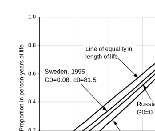
₀.

Figure 1: Lorenz curves for three female populations with different average levels and age distributions of mortality.

Sources: Data for computations for Sweden are extracted from The Berkeley Mortality Database. Our own estimates are based on the original Goskomstat’s data on deaths and population by age for Russia. Life table for Bangladesh is taken from Matlab Report (1996).

2.3 Gini coefficient

Various measures of inequality try to express in different ways a degree of inequality or variability as one number. Some of them are directly based on the Lorenz curve, and others are not. Gini coefficient is the best known and the most widely used measure of divergence based on the Lorenz curve. It is defined as an area between the diagonal and the Lorenz curve, divided by the whole area below the diagonal (equal to 1/2). Analytically it can be expressed as

∫

Φ ⋅ −

= 1

0

0 1 2 (p)dp

G , where p=F(x) (4)

0.0 0.2 0.4 0.6 0.8 1.0

0.0 0.2 0.4 0.6 0.8 1.0

Proportion in population

P

ropor

ti

on

in pe

rs

on-y

ear

s

of

l

if

e

Matlab (Bangladesh), 1995 G0=0.22; e0=63.5

Russia, 1995 G0=0.13; e0=71.8 Sweden, 1995

G0=0.08; e0=81.5

Hanada (1983) showed that definition (4) together with (1)-(3) leads to

∫

∞

⋅ −

=

0 2 2

0 [ ( )]

)] 0 ( )[ 0 (

1

1 l x dx

l e

G (5)

Sometimes it is impossible to get mortality data for the full range of ages. For example, mortality data could be unreliable at infant ages or at old ages. Often, in studies combining inter-individual inequalities with inter-group (social class) inequalities in length of life (see section 4), group-specific data on mortality are available only for a limited range of ages (e.g. working ages). Therefore, one might want to measure the inequality in age at death for ages above 15 (denoted as

15

G ) or between 20 and 65 (denoted as

65 | 20

G ).

Formula (5) can be re-written for the range of ages [x, X]

∫

⋅ −

=

X

x X

x l t dt

x l X x e

G| ₂ [()]2

)] ( )[ | (

1

1 , (5a)

where the temporary life expectancy is ₌

∫

X

x dt t l x l X x

e ( )

) (

1 ) |

( (Arriaga, 1984).

Gini coefficient varies between the limits of 0 (perfect equality) and 1 (perfect inequality). For a length-of-life distribution, it is equal to zero if all individuals die at the same age, and equal to 1 if all people die at age 0 and one individual dies at an infinitely old age.

There are several other ways to define Gini coefficient apart from the geometric definition (4). All of them are equivalent (Anand, 1983). The definition by Kendall and Stuart (1966) is especially helpful for understanding the nature of this measure.

∫∫

∞ ∞

− =

0 0

0 | | ( ) ( ) 2

1

dxdy y f x f y x G

µ

(6)

∑∑

_{= =}

−

=

n

i n

j

j i

x

x

e

l

G

1 1 0 0

2 0

)

(

2

1

_{. (6a)}

This expression can be re-written in terms of the standard life table functions as

∑∑

= =

−

⋅

⋅

=

ω ω

0 0 0 0

2 0

)

(

2

1

x y

y

x

d

x

y

d

e

l

G

, (6b)

where

x

and

y

are the average ages at death for the elementary age intervals [x, x+1) and [y, y+1), respectively.

Formula (7) is simple to understand, but is not easy to apply in practical calculations. In this respect, it is preferable to use Hanada’s formula (5). As a construct,

this formula is quite similar to the one for life expectancy

∫

∞

⋅ =

0

0 ( )

) 0 (

1

dx x l l

e . The task

is to estimate the area under the curve _{[ xl( )]}2 _{similarly to the area under curve}

) ( x

l for

life expectancy. This similarity helps to find a simple way for calculation of G0 from discrete data (see section 3).

Formulae (6), (6a) and (7) make it clear that Gini coefficient is a mean-standardized measure. It varies from 0 to 1 and reflects relative inter-individual inequality. Such measures are also called indices. For some reasons one might be interested in absolute inter-individual differences in length of life. A respective

measure, denoted abs

G0 , can be obtained from formulae (5) or (6) by removing life

expectancy from the denominator (Note 2). It is equal to the average inter-individual difference in length of life and is measured in years. The Hanada’s formula (5) yields

∫

∞

⋅ − = ⋅ =

0 2 2

0

0 [( )]

)] 0 ( [

1 ) 0 ( ) 0

( l x dx

l e e G

Gabs (7)

The present paper focuses on the relative Gini coefficient, but sections 3 and 4 also

show how to compute and decompose abs

2.4 Basic properties of inequality measures

The following basic properties are desirable for any index of income inequality (Anand, 1983):

(a) population-size independence (or relativity principle), that is, the index does not change if the overall number of individuals changes with no change in proportions of individual incomes;

(b) mean or scale independence, that is, the index does not change if everyone’s income changes by the same proportion;

(c) Pigou-Dalton condition (or transfer principle), that is, any transfer from a richer to a poorer individual that does not reverse their relative ranks reduces the value of the index.

Satisfaction of these three conditions guarantees that an index of income inequality will correctly reflect the Lorenz-dominance (Anand, 1983). That is to say that in a comparison of two income distributions it will have a smaller value for the income distribution, which dominates another distribution.

Gini coefficient satisfies basic conditions (a) to (c) (Anand, 1983, Goodwin and Vaupel, 1985) and, therefore, correctly reflects the Lorenz-dominance among distributions of length of life. Note values of G0 in Figure 3 as an example.

Let us briefly consider a selection of other measures of inequality, which have already been applied elsewhere to distributions of length of life (Wilmoth and Horiuchi, 1999, Anand et al., 2001, Anand and Nathikesan, 2001), in light of basic properties (a) to (c).

The interquartile range (IQR) (see appendix 1 and Wilmoth and Horiuchi, 1999 for its exact definition) satisfies conditions (a) and (b), but does not satisfy the Pigou-Dalton condition (c). Indeed, an inter-individual transfer of years of life between two individuals will not change the IQR if both ages at death are either inside the quartile limits, both of them are higher than the upper limit, or both of them are lower than the lower limit. It means that the IQR ignores a change in distribution of deaths within certain age ranges if the total death numbers for each of these ranges do not change. For example, if x75=60 years (25,000 of 100,000 die at ages under 60) then it does not matter whether 20,000 die at ages under 15 and 5,000 die at ages from 15 to 59 or if 5,000 die at ages under 15 and 20,000 die at ages from 15 to 59.

not standardized by the average life expectancy and, therefore, do not satisfy condition (b) of the mean- or scale- independence. Indeed, if all ages at death are multiplied by factor s then the variance of ages at death changes by factor s2 and STD changes by factor s. This means that the measure can change even if the distribution remains unchanged, but mean value changes (Note 3).

Unlike VAR, the variance of the logarithm of length of life (VarLog) (see appendix 1 for definition) is scale- and mean- independent, but it does not satisfy the Pigou-Dalton condition for ages above µˆe (where e is the base of the natural logarithm) (Anand, 1983).

The Theil entropy index (T) is based on the notion of entropy in information theory (see appendix 1, Anand, 1983, and Theil, 1967). It satisfies all basic properties (a) to (c), but it is more difficult to understand or to interpret it in comparison to G, IQR or STD. Theil interprets T as "the expected information of a message which transforms population shares into income shares" (Theil, 1967, p. 95 cited by Anand, 1983, p. 309). Different inequality measures are characterized by different sensitivity to changes in different sections of the length-of-life distribution. In practice, their sensitivity to changes in infant mortality is especially important. A.Atkinson constructed an inequality index with degrees of aversion to inequality expressed in an implicit form by a special parameter of aversion (Atkinson, 1970). Its minimum value of 0 means that all ages have the same weight in the inequality index. Higher values of the aversion parameter attach increasingly greater weights to earlier years of life (Anand et al, 2001). Basic properties (a) to (c) and information on sensitivity to changes in tails of the length-of-life distribution suggest how a given measure of inequality will behave when applied to real mortality data. The following section shows that differences in properties of inequality measures have implications for empirical results.

3. Empirical trends in Gini coefficient and other measures of

inequality and judgements about direction of changes in inequality

Wilmoth and Horiuchi (1999) showed that for several industrialized countries, there is high correlation between long term trends in various measures of inequality. However, this result does not mean a full agreement between the directions of all temporal changes in various measures of inequality.

mortality decreases at infant age and increases at adult ages, then Atkinson indices with high aversion parameters show an increase in inequality, while all other measures of inequality show a decrease. This section provides additional empirical evidence of the same nature by looking at similarities and dissimilarities among temporal changes in G0 and four other measures of inequality in length of life.

We consider trends in the selected measures of inequality for male populations of the USA and Russia since the 1950s. These countries and time periods have been selected as demonstrative ones after extensive exploratory analyses for nine industrialized countries over longer time periods.

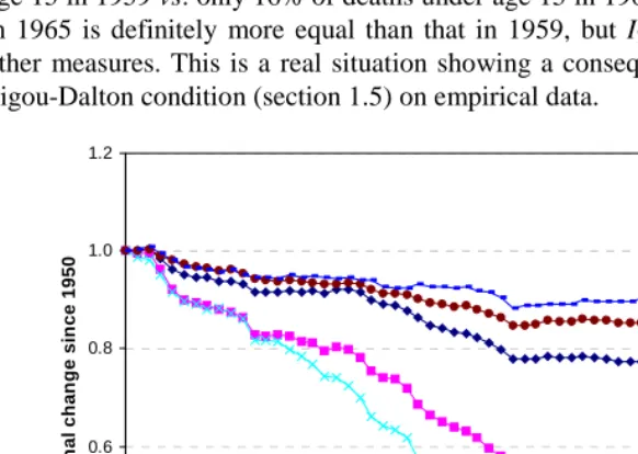
Figure 2a suggests a remarkable similarity among proportional changes in the Gini coefficient, the standard deviation, the variance of log-life, the Theil entropy index, and the interquartile range for males in the USA from 1950 to 1995. All trends decline in response to transfers of deaths from younger to older ages and growing concentration of deaths at old ages.

Age-decompositions of changes (not shown here) demonstrate that differences between measures in the pace of temporal decline (steepest changes in VarLog and slowest changes in IQR) are mostly due to their varied sensitivity to decreasing infant mortality. VarLog continues to decrease in the 1960s in spite of mortality stagnation at adult ages and also in the 1980s-90s when all other measures of inequality stabilize. T also declines steeply in the 1950s due to declining infant mortality, but it becomes sensitive to changes at adult ages after 1960 when the number of infant deaths becomes low.

IQR, G0 and STD tend to stabilize in the 1960s due to mortality stagnation and also in the 1980s-90s. Reasons for the most recent stabilization are considered in section 5. IQR is also quite stable during the 1970s, while G0 and STD decrease. Once again, this difference is attributable to a varied sensitivity to mortality decline at young ages.

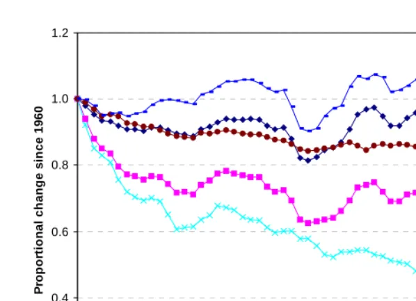
Russian mortality data provides an excellent opportunity for empirical testing of the inequality measures. This is due to the remarkable diversity among mortality trends for different age groups. In 1959-2000, mortality in infancy and childhood was decreasing, except for a short period of 1971-74. Mortality at ages from 15 to 69 was continuously increasing, except for a short period of sudden decline in 1985-87, and mortality at ages above 70 was mostly increasing at a slow pace (Shkolnikov, Meslé and Vallin, 1996). Life expectancy at birth increased from 1959 to 1964, and has continuously decreased since then, except 1985-87, when it increased.

changes at adult ages. The trend in G0 is similar to that in T, with a less significant decrease from 1959 to 1965 and a greater magnitude of variations after 1985.

The trend in IQR deserves special attention. Interestingly, IQR increases between 1962 and 1970, while G0 and all other measures of inequality decrease. For a better understanding of this fact, it is useful to compare two time points with almost the same values of IQR, x75 and x25: 23.8, 54.5, and 78.3 years in 1959, respectively, and 23.7, 54.6, and 78.3 years in 1968, respectively. The number of life table deaths under age 55 is almost the same in 1959 as in 1968 (25,503 vs. 25,410 with radix 100,000). However, these deaths are distributed differently among ages under 55, with 26% of deaths under age 15 in 1959 vs. only 16% of deaths under age 15 in 1968. Age-distribution of deaths in 1965 is definitely more equal than that in 1959, but IQR remains invariant, unlike other measures. This is a real situation showing a consequence of the violation of the Pigou-Dalton condition (section 1.5) on empirical data.

Figure 2a: Proportional changes in Gini coefficient (G0), standard deviation (STD), variance of log-life (VarLog), Theil entropy index (T), and interquartile range (IQR) for males in the USA in 1950-97. (Level in 1950 is taken as 1).

Source: data for computation are extracted from The Berkeley Mortality Database (2001), originally constructed by the Office of the Actuary of the Social Security Administration.

0.2 0.4 0.6 0.8 1.0 1.2

1950 1960 1970 1980 1990 2000

Year

P

ropor

ti

ona

l c

h

a

nge

s

inc

e

1950

G

T

VarLog

STD

Figure 2b: Proportional changes in Gini coefficient (G0), standard deviation (STD), variance of log-life (VarLog), Theil entropy index (T), and interquartile range (IQR) for males in Russia in 1959-2000. (Level in 1959 is taken as 1).

Source: data for computation are extracted from the original Goskomstat’s annual files on deaths and mid-year population estimates.

The trend in STD shows a low variation across years relative to the starting year. In the case of Russia it appears that changes in the distribution of deaths by age lead to relatively minor changes in the sum of squares of deviations from the continuously

declining average length of life. The coefficient of variation, equal to STD/e0,

experiences significantly greater magnitudes of proportional changes from 1959 to 2000 (not shown here).

Let us make another comparison of the length-of-life distributions for Russian men between 1965 and 1975. There is less inequality in 1975 compared to 1965 in terms of VarLog and STD, more inequality in 1975 compared to 1965 in terms of IQR and G0 and almost no difference between 1965 and 1975 in terms of T. This suggests that the choice of measure can change a conclusion about the direction of changes in inequality.

There is no reason to claim that one of all possible measures of inequality is the best. This claim is impossible in economics or statistics, and it is equally impossible in demography. Different measures emphasize different aspects of length-of-life

0.2 0.4 0.6 0.8 1.0 1.2

1959 1969 1979 1989 1999

Year

P

rop

o

rtio

n

al

ch

ang

e

s

in

c

e

19

60 G

T

VarLog

STD

distributions. Relevance of their application depends on concrete purposes of analysis. On the other hand, some measures are used more widely than other ones because they fit better to typical situations and are easy for computation.

Theoretical considerations of the previous section, and empirical findings of this section, show that a violation of one of the basic properties (a) to (c) is a worrying signal. In this connection, one might prefer to use G0, T and VarLog rather than IQR or STD.

VarLog is also not free from theoretical disadvantages (Anand, 1983), since it does not satisfy the Pigou-Dalton condition for the whole range of ages (see section 1.5). In addition, it is so sensitive to changes in infant mortality that it does not react significantly, even to large changes at adult ages if infant mortality continues to decline. T has no disadvantage in comparison to G0, both from the theoretical or empirical sides. But it seems that this entropy-based measure is quite difficult for use in both understanding and interpretation.

Finally, in this study we favor Gini coefficient. It satisfies the basic properties in (a) to (c). Unlike many other inequality measures (shown and not shown here), it is not extremely sensitive to redistributions at early ages of life and reflects the changes at adult ages well.

Gini coefficient is an intuitively meaningful measure, which can be understood from its definitions (section 1.4) and from the analogy with income.

The following section shows how Gini coefficient can be computed from life table data.

4. Computation of Gini coefficient from complete and abridged life

tables

The availability of life tables for a population presumes an ability to estimate the

integral

∫

∞

0 ) (x dx

l from discrete data. It would also help to estimate the integral

[ ]

∫

∞

0 2 ) (x dx

l .

In a complete life table with l₀ =1 the life expectancy at birth is estimated as

[

]

∑

∑

∑∫

+ = = + + − +

=

x

x x x x x

x x

l l A l L dt t x l

e ( ) 1 ( 1)

1

0

For an elementary age interval [x, x+1), parameter A is the average share of the_x interval lived by individuals, who die within the interval. These parameters are known

from the life table

1 1 ) 1 / ( + + − − = x x x x x l l l L A .

Let us assume that the integral

∫

[

]

∞

0 2 ) (x dx

l can be expressed in a similar way

[

]

_∑

[

]

∑∫

+ = + + − + x x x x x x l l A l dt t x

l( ) ( ) ˆ (( ) ( 1)2) 2

2 1 1

0

2 _{. (8)}

Unknown parameters Aˆ_x are to be estimated. For ages x>0survival function

) (x t

l + can be reasonably well described by a parabola within the elementary age

interval 0≤t≤1. A parabola having the value l_x at t=0 and the value l_x+1 at t=1

with the integral from 0 to 1 equal to L is_x

)

1

(

)

(

6

)

(

)

(

x

+

t

=

l

+

l

₊₁

−

l

t

+

C

l

₊₁

−

l

t

t

−

l

_{x x x x x x} , (9)

where

2

1

−

=

x x

A

C

.

It is possible then to determine a polynomial of the fourth degree for the function

of our interest

[

]

2

) (x t

l + (see Appendix 2 for more details), and to derive the expression

for x

Aˆ by using (8)

x x x x x x q C q C q A − − − + − = 2 ) 5 6 2 ( 3 2 1 ˆ (10)

For a simple case with life table deaths evenly distributed within an elementary

age interval

2

1

=

x

A

and C_x =0 and formula (10) yields

It implies that

2

1

ˆ

₌

x

A

if q_x =0 and

3

1

ˆ

₌

x

A

if q_x =1. If the probability of death

is low (which is true for most of the ages in a complete life table) then the difference between _Aˆ_x and A is also very small. At old ages, where the probability of death is_x higher, the decrease in

[ ]

2

) ( x

l becomes considerably steeper than the decrease in l( x)

and the deviation of x

Aˆ from A becomes greater. x Aˆx tends to be smaller thanA ,x

consequently, a numerical integration (8) of the function

[ ]

2

) ( x

l by using the original life

table A instead of "true" parameters _x Aˆ_x would result in some underestimation of G .0

Formula (10) is also valid for an abridged life table if for an elementary age

interval [x,x+n) parameter A is defined as _x

n x x n x x n l l l n L + + − − ) /

( _{and, therefore varies}

between 0 and 1.

Formula (10) would not work in a proper way for x=0 because during the first year of life l( x) falls more steeply than can be predicted by a quadratic polynomial. The use of the formula by J.Borgois-Pichat (1951) instead of a parabola (Appendix 3), solves the problem for age 0 and results in

      + ⋅ + − = 0 0 0 0 0 2 831 . 0 3 1 ˆ q A q A

A . (11)

Let us, lastly, find a solution for an open-age interval. For many populations mortality data running up to the highest ages are not available. For example, in the WHO Mortality Database (2001), the last age group is 85+ for almost all countries and calendar years. Fortunately, The Berkeley Mortality Database (The Berkeley Mortality Database, 2001) provides 335 complete life tables for Japan, France, Sweden, and the USA with single-year age groups running up to 110. Mortality data by single-year age group for ages 85-110 provide the possibility to find a solution for the last age group 85+.

For an elementary age interval

[

x

,

x

+

n

)

∫

+ = ⋅ + + ⋅ − +

=x n x n x x x n x x

nL l(t)dt n l n A (l l ). For the open-ended interval 85+ l∞ =0

and A₈₅₊ can be defined as

∫

∞

+ = ⋅ =

85

85 85

85 ( )

1 e dx x l l

A (Note4).

[

]

∑

∫

₌ + +

∞

+ = ⋅ ≅ + −

109

85

2 1 2 2

1 2

85 85

2 2

85

85 ( ) ˆ (( ) ( ) )

) (

1 )]

( [ ) (

1 ˆ

x

x x x

x A l l

l l

dx x l l

A . Having the

values of l and _x A and computing _x Aˆ_x from (10), one can obtain A85+. The general

relationship between _Aˆ₈₅₊ and A₈₅₊ =e₈₅ can be estimated on the basis of the 335 life tables, by means of linear regression (Note 5). It returns the following equations:

85 85 0.440 0.680

ˆ _e

A =− + ⋅ (for women),

85 85 0.227 0.626

ˆ _e

A =− + ⋅ (for men) (12)

Formulae (10), (11), and (12) give a set of parameters Aˆ_x for the numerical

integration of the function

[ ]

2

) ( x

l . After this stage is completed it is easy to calculate

0

G or G0absaccording to formulae (5) and (7).

Table 1 shows the magnitudes of errors depending on the type of input data (complete life tables, abridged life tables with ages running up to 110 or abridged life tables with the last age 85+) and the method of computation (with A or with _x Aˆ_x) for

Swedish life tables. These data for the years 1861, 1900, 1920, 1940, 1960, 1980, and 1995 are taken from The Berkeley Mortality Database (2001). Values of Gini coefficient computed from complete life tables with the last age 110, and adjusted Aˆ_x,

are considered as "exact" estimates. Abridged life tables and abridged life tables with the last age group 85+ are made from complete life tables in a conventional way. Table 1 suggests that if the data of complete life tables with the last age 110 are available, then it is not that important whether the original A or adjusted _x Aˆ_x are used. Although

in the former case where G estimates are systematically lower than the "exact" ones,₀ the deviation is very small. As was mentioned before, the errors of approximating models are higher at infant and old ages, where functions

l

(x

)

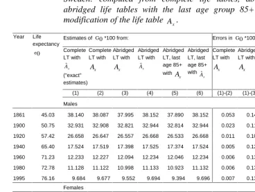
and especially 2

Table 1: Life expectancy at birth and different estimates of Gini coefficient for Sweden: computed from complete life tables, abridged life tables, abridged life tables with the last age group 85+ with and without modification of the life table

x

A .

Estimates of G0*100 from: Errors in G0*100 estimates:

Complete LT with

x Aˆ

("exact" estimates)

Complete LT with

x A

Abridged LT with

x A

Abridged LT with

x Aˆ

Abridged LT, last age 85+ with

x A

Abridged LT, last age 85+ with

x Aˆ

Complete LT with

x A

Abridged LT with

x A

Abridged LT with

x Aˆ

Abridged LT, last age 85+ with

x A

Abridged LT, last age 85+ with

x Aˆ

(1) (2) (3) (4) (5) (6) (1)-(2) (1)-(3) (1)-(4) (1)-(5) (1)-(6) Year Life

expectancy

0 e

Males

1861 45.03 38.140 38.087 37.995 38.152 37.890 38.152 0.053 0.145 -0.012 0.250 -0.012 1900 50.75 32.931 32.908 32.821 32.944 32.814 32.944 0.023 0.110 -0.013 0.117 -0.013 1920 57.42 26.658 26.647 26.557 26.668 26.533 26.668 0.011 0.101 -0.010 0.125 -0.010 1940 65.40 17.524 17.519 17.398 17.525 17.374 17.524 0.005 0.126 -0.001 0.150 0.000 1960 71.23 12.233 12.227 12.094 12.234 12.046 12.234 0.006 0.139 -0.001 0.187 -0.001 1980 72.78 11.128 11.122 10.998 11.133 10.923 11.132 0.006 0.130 -0.005 0.205 -0.004 1995 76.16 9.684 9.677 9.552 9.694 9.394 9.696 0.007 0.132 -0.010 0.290 -0.012

Females

1861 48.78 35.436 35.403 35.319 35.457 35.309 35.457 0.033 0.117 -0.021 0.127 -0.021 1900 53.62 30.984 30.970 30.872 30.990 30.855 30.989 0.014 0.112 -0.006 0.129 -0.005 1920 60.11 24.627 24.620 24.516 24.627 24.475 24.626 0.007 0.111 0.000 0.152 0.001 1940 68.14 15.473 15.468 15.339 15.473 15.302 15.473 0.005 0.134 0.000 0.171 0.000 1960 74.87 10.382 10.376 10.237 10.387 10.129 10.385 0.006 0.145 -0.005 0.253 -0.003 1980 78.85 9.157 9.151 9.019 9.163 8.692 9.172 0.006 0.138 -0.006 0.465 -0.015 1995 81.45 8.337 8.331 8.192 8.339 7.630 8.381 0.006 0.145 -0.002 0.707 -0.044 Sources: Data for computations are extracted from The Berkeley Mortality Database (2001).

The values of G computed with ₀ A are relatively imprecise for abridged life_x tables, especially if the last age group is 85+ (Table 1). Markedly, the error has tended to increase quite significantly in the last five decades because the proportion of deaths occurring at ages above 85 has been increasing steeply.

Presented in Table 2 are the maximum relative deviations of five different estimates of G0⋅100 from the "exact" estimates for 335 life tables taken from The

Berkeley Mortality Database (for France, Japan, Sweden and the USA). It confirms the results of Table 1 on the basis of a large number of mortality schedules. Additionally, Table 2 shows that in the most recent years (low values of G ) the estimates computed₀ from female abridged life tables, with the last age group 85+ using

x

slightly upwards from their "exact" values. This indicates that the use of ₊ 85

ˆ

A for the

computation of G can not replace real mortality rates at ages above 85 if the₀

proportion of life table deaths at age 85+ continues to increase. At present, the respective error is small, but it will increase with time and in the future it will be necessary to use mortality data for ages above 85.

In all cases the use of modified parameters x

Aˆ reduce errors to a large extent and

in all cases they become small. In order to re-check our prior results on the data, which

had not been used to derive formulae (12) for estimating ₊

85

ˆ

A , we made another

comparison. First, we computed G0⋅100 values from 89 complete life tables (from the

Human Life-Table Database (2002)) with the last age group from 90 to 110 (mostly 100-105) for a diverse set of countries and years ("exact" estimates). Second, we computed two estimates of G0⋅100 using A or x Aˆx from 89 abridged life tables with the last age 85+, corresponding to the complete life tables. For men, the average difference from the "exact" estimates of G0⋅100 was 0.189 using A -estimates andx

only 0.014 using x

Aˆ -estimates. For women, the equivalent figures were 0.291 and

0.026, respectively.

Table 2: Maximum relative errors of the estimates of ₁₀₀

0⋅

G computed from

complete life tables, abridged life tables, abridged life tables with the last age 85+ with and without modification of the life table by level of "exact"

100 0⋅

G , in per cent.

Ranges of "exact" values of

100

0⋅

G

Number of life tables

Complete life tables,

x

A

Abridged life tables,

x

A

Abridged life tables,

x

Aˆ

Abridged life tables with the last age 85+,

x

Aˆ

Abridged life tables with the last age 85+,

x

Aˆ

Males

< 15 145 -0.06 -1.40 0.06 -3.78 0.08

15 ” < 20 66 -0.05 -0.85 0.03 -1.08 0.03

20 ”< 25 38 -0.06 -0.59 0.04 -0.73 0.03

25 ”< 30 40 -0.08 -0.44 0.04 -0.49 0.04

30 ” 29 -0.14 -0.40 0.06 -0.41 0.06

35 ” 17 -0.27 -0.94 0.53 -0.94 0.53

Females

< 10 72 -0.07 -1.78 0.09 -12.40 1.18

10 ” < 15 113 -0.04 -0.84 0.04 -1.30 0.03

15 ” < 20 35 -0.05 -0.60 0.04 -0.88 0.04

20 ”< 25 43 -0.07 -0.46 0.05 -0.57 0.04

25 ”< 30 41 -0.13 -0.40 0.05 -0.43 0.05

30 ” 31 -0.14 -0.38 0.05 -0.39 0.05

5. Decomposition of a difference between two values of Gini

coefficient

5.1. Age

When analyzing changes in life expectancy over time or its variations across countries it is useful to be able to decompose observed differences by age and cause of death. This gives one the opportunity of linking variations in overall life expectancy with variations in elementary age-specific mortality rates. For a similar reason the idea of decomposition of differences between two Gini coefficients arises. The age-components would show to what extent differences in elementary mortality rates at different ages influence the overall difference in degrees of inequality in length of life.

The discrete method for the decomposition of a difference between two life expectancies by age was independently developed in the 1980s by three researchers from Russia, the USA, and France (Andreev, 1982, Arriaga, 1984, Pressat, 1985). The formula of decomposition by E.Andreev is exactly equivalent to that by R.Pressat. The formula by E.Arriaga is written in a slightly different form, but is actually equivalent to the formula by Andreev and Pressat (Shkolnikov et al., 2001). A continuous version of the method of decomposition by age was developed by Pollard (1982).

All of these methods are based on the idea of standardization or replacement (Kitagawa, 1964). If there are two populations under consideration then mortality rates of the first population are to be replaced in an age-by-age mode by mortality rates of the second population, or vice versa (Andreev, Shkolnikov, Begun, 2002). The contribution of a particular age group

x

to the overall difference in life expectancy can be computed as the difference between life expectancy of the first population and the life expectancy of the first population after replacement of the mortality rate at age

x

by the respective mortality rate of the second population.

First, we apply this general algorithm to a difference between e₀ values and

demonstrate that it leads to the conventional formula of decomposition. We then apply the same approach again to develop the formulae for decomposition of the difference between G values.₀

Let µ[ x] _{be the force of mortality function equal to the force of mortality of the}

second population µ′(t) if t≤x and equal to the force of mortality of the first population µ(t) if t>x. Then the difference in life expectancy at birth produced by replacement of force of mortality from 0 to

x

is

x x x x x x

x =e ( )−e0 =(L0′| −L0| )+(l′ −l )⋅e ]

[ 0 ,

0

µ

where ₌

∫

x

x l t dt L

0 |

0 ( ) . The first additive term in the expression is the effect of

replacement at ages under

x

; the second additive term is the effect of replacement at ages under

x

on length of life after age

x

. If the range of ages is divided into n intervals [x_i,x_i+1) then the overall difference between the two life expectancies can be decomposed into age-specific contributions as

∑

∑

= − =

=

−

=

−

′

₊ n

i i n

i

x

xi i

e

e

0 1 0 , 0 , 0 0

0

(

δ

1

δ

)

δ

(14)

i

δ

can be regarded as a contribution of an elementary age interval [x_i,x_i+1) to the overall difference between life expectancies at birth. Using (14) and (13) we easily come to the conventional formula of decomposition by Andreev and Pressat

∑

= + + +

−

′

′

−

−

′

′

=

−

′

n i x x x x x

xi

e

i

e

i

l

i

e

i

e

i

l

e

e

0 0

0

[

(

)

1

(

1 1

)].

Components

i

δ

can be presented in a more general way as

) ( ) ( [ ] 0 ] [ 0 1 i i x x

i =e Μ −e Μ

+

δ

, (15)

where Μ[xi] _{is a vector of age-specific mortality rates with elements}

x

m′ for x≤x_i and

x

m for x>x_i. In fact, formula (15) can be considered as a general procedure for decomposition by age of a difference between two aggregate measures (Andreev, Shkolnikov and Begun, 2002). It determines a stepwise replacement of one mortality schedule by another one, beginning from the youngest and proceeding to the oldest age group. Discussion about this and other orders of replacement in respect to the age-decompositions can be found elsewhere (Pollard, 1988, Das Gupta, 1994 and 1999, Horiuchi, Wilmoth and Pletcher, 2001, Andreev, Shkolnikov and Begun, 2002).

A formula for age-components for the difference between two

0

G values can be developed by using definition (5) in a way similar to (13)-(14). The difference induced by mortality replacement at age

x

and younger ages can be expressed as

x x x x x x x x l e e l e G G ′ + ′ ′ + ′ − = − Μ = | 0 2 | 0 0 0 0 ] [ 0 , 0 ) ( ) (

θ

θ

θ

where

∫

∞

= x x

x l t dt

l

2 2 [( )] )

( 1

θ

, ₌

∫

x

x l t dt

0 2 |

0 [( )]

θ

and ₌

∫

x

x l t dt e

0 |

0 ( ) .

The decomposition of the difference in between two Gini coefficients by age group similar to (14) is

∑

∑

= −

=

=

−

=

−

′

₊ n

i i n

i

x

xi i

G

G

0 1

0

, 0 , 0 0

0

(

ε

1

ε

)

ε

(17)

and a general procedure for the computation of age-specific components of the difference is

) ( )

( 0 [ ]

] [ 0

1 i

i x

x

i =G Μ −G Μ

+

ε

(18)

Similar formulae for the age-components of the difference between two abs

G₀ values are given in appendix 4.

Formulae (16) and (17) allow a difference between two Gini coefficients to be split according to age groups. Similar to life expectancy (Andreev, 1982, Pressat, 1985), the results of decomposition are not exactly the same for the difference G₀′−G₀in comparison to the difference G₀ −G₀′. That is to say that it does matter which mortality schedule is the basic one, which has to be replaced by another one. A conventional way to avoid this problem is to perform the decomposition (17) twice, and then to average the resulting age-specific components. In the present paper this technique is used in all decompositions.

Formulae (16) and (17) are analytical expressions, permitting a direct computation. Numerical integration for values of

x

θ and

x

| 0

θ can be completed by using the technique

developed in the previous section (usage of the adjusted x

Aˆ instead of the life table

x

A ).

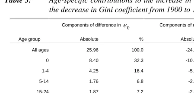
Table 3: Age-specific contributions to the increase in life expectancy at birth and the decrease in Gini coefficient from 1900 to 1995: USA, men*

Components of difference in

0

e Components of difference in ₁₀₀

0⋅

G

Age group Absolute % Absolute %

All ages 25.96 100.0 -24.02 100.0

0 8.40 32.3 -10.99 45.7

1-4 4.25 16.4 -5.50 22.9

5-14 1.76 6.8 -2.15 9.0

15-24 1.87 7.2 -2.00 8.3

25-39 2.94 11.3 -2.61 10.9

40-64 4.30 16.6 -1.91 7.9

65+ 2.44 9.4 1.14 -4.7

* e0 (1900)=46.4, e0 (1995)=72.73 G0 (1900)=36.73, G0 (1995)=12.71

Sources: Data for computations are extracted from The Berkeley Mortality Database (2001). Life tables for the United States are based on those constructed by the Office of the Actuary of the Social Security Administration.

Table 3 shows the results of the decomposition of increase in life expectancy at birth and of the decrease in the Gini coefficient in the USA between 1900 and 1995. The total increase in life expectancy at birth is 26 years for men and 30 years for women, and the total decrease in G0⋅100is about 24 for both sexes. 55% of the overall

increase in life expectancy is due to a decrease in mortality at ages 0-14. A 35% increase in life expectancy for men and 39% for women is due to a decrease in mortality at ages 15-64, and a further 9% increase for men and 17% for women is due to a decrease in mortality at ages 65 and older. The overall decrease in Gini coefficient is distributed somewhat differently. The proportion of the decrease due to the youngest age group 0-14 is higher than that for life expectancy (78% for men and 70% for women). The proportion of the medium age group is somewhat lower (27% for men and 37% for women), and the oldest age group produces a negative contribution of – 5%.

by avoiding deaths. This is similar to an income redistribution, with the poorest gaining more additional income than the rich.

5.2. Age and cause of death

With the help of definition (5), formula (16) can be re-written without e0|_x and

θ

0|x as

x x x x x x x x x

l

e

e

l

e

l

l

e

−

′

′

+

′

′

+

′

′

−

′

−

=

0 2 2 0 0 0 , 0

)

(

)

(

θ

θ

θ

θ

ε

(19)

The following relations are true for a small ∆x:

lx+∆x =lx(1−

µ

x∆x),

e

x+∆x

= − −

e

x

(

1

µ

x x

e

)

∆

x

,

θ

x+∆x =

θ

x− −(1 2

µ θ

x x)∆x.

Applying (17) and (19) to a small age interval

[

x

,

x

+

∆

x

]

after some

transformations, one can yield

. ) ( )]} ( [ 2 )] ( ) ( [ { )] ( [ ) ( 0 2 0 2 0 , x x x x x x x x x x x x x x x x x x x x x

x e l l e l e e

e e l e l x η µ µ θ θ θ θ µ µ ε λ ′ − = = ′ − ′ + ′ ′ − ′ − ′ + ′ ′ − ′ + ′ ′ ′ − = ∆ = +∆ (20)

Integrating (20) from

x

_i to

x

_i+1 yields

∫

∫

∑ ∫

+ + + + + + = = − ′ ≅ − ′ ⋅ = 1 1 1 1 1

1 ( ) ( | | )

1 , i i i i i i i i i i i i x x t x x x x x x m j x x t t t t x

x λdt µ µ ηdt m m ηdt

ε .

If there are m causes of death, then

∑

= = m j j x x 1 , µ µ and

∫

+

∑

+ + + = ′ − ⋅

≅ 1 _{1 1}

1 1 , | , | , ( ) ( ). i i i i i i i i x x m j j x x j x x t x

x ηdt m m

ε

If in each age group [x_i,x_i+1)

1

1 |

|i+ ≠ ′i i+

ix xx

x m

this age group are simply 1 1 1 1 1 1 , | | , | , | , , + + + + + + − ′ ⋅ ′ −

= _{i i}

i i i i i i i i i

i x x

x x x x j x x j x x j x x m m m m

ε

ε

,

otherwise a numerical integration would be necessary to compute cause-specific components according to

∫

+ + +

+ ≅ ⋅ − ′

1

1 1

1, ( ) ( | , | , ).

, i i i i i i i i x x j x x j x x t j x

x ηdt m m

ε

Similar formulae for age- and cause-specific components of a difference between two

abs

G0 values are given in appendix 4.

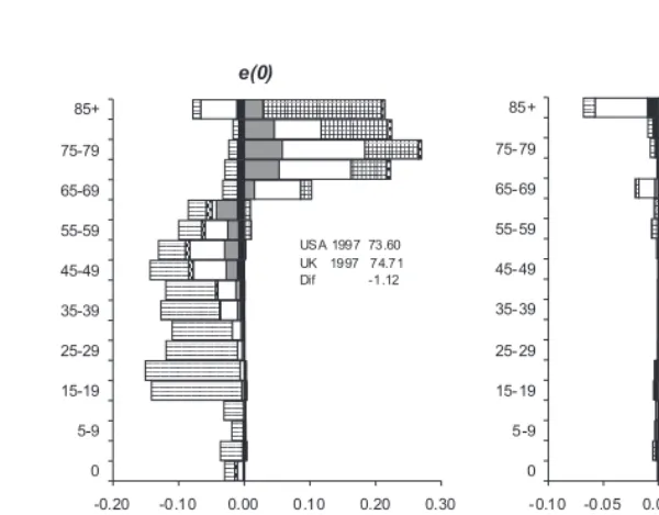
A comparison between the USA and the UK male life expectancies at birth and the USA and the UK Gini coefficients in the year 1997 is given as an example of decomposition by age and cause of death (Figure 3). The life expectancies of men are very similar in both countries. The difference is only one year in favor of the UK (or 1.4%). However, there is a significant 16% difference in the Gini coefficients with less inequality in length of life in the UK.

Figure 3 shows age- and cause-specific components of these differences. The advantage of the UK in male life expectancy (left panel of Figure 3) is mostly due to lower mortality rates by external causes of death (accidents and violence) at ages from 15 to 50 and, to some extend, to lower mortality rates by circulatory disease and cancers at ages from 40 to 59. However, this advantage is almost balanced by the effects of lower mortality in the USA at ages above 65 by circulatory and respiratory diseases and cancers.

The weight of external causes of death at young adult ages is higher for the UK-USA difference in the Gini coefficients (right panel of Figure 3) than that for the difference in life expectancies at birth. In addition, low mortality at old ages increases the level of the Gini coefficient in the USA in comparison to the UK.

Elimination of causes of death is another method for analyzing the influence of causes of death on life table measures. A conventional procedure of building the "associated" single decrement life table can be applied (Chiang, 1968, Preston et al., 2001). Gini coefficient can be computed from this table with modified Aˆ_x (as described

in section 1).

Figure 3: Decompositions of the differences in life expectancy at birth and in Gini coefficient between the UK and the USA by age and cause of death: male populations, 1997.

Sources: Data for computations are extracted from the WHO Mortality Database (2001)

for women in the UK in 1951-1996. For the majority of causes of death, elimination leads to a decrease in G . There are two exceptions: cardiovascular diseases during the₀

whole period, and respiratory diseases after 1973. Their elimination increases G₀

Figure 4: Effects of elimination of causes of death on G for women in the UK in₀ 1951-1996

Sources: Data for computations are extracted from the WHO Mortality Database (2001)

In the 1950s, the elimination of perinatal causes and congenital anomalies could have lead to the greatest decrease in G among other causes of death. By the 1990s, the₀ effect of this major cause of infant death had been greatly reduced. The same has happened to other common causes of mortality in childhood (infectious and respiratory diseases). The elimination effects of cancers and external causes of death have been relatively stable in time.

At present, eliminating external causes of death, can produce the greatest decrease in G0 for women in the U.K.

-2.5 -2.0 -1.5 -1.0 -0.5 0.0 0.5 1.0 1.5 2.0

1950 1960 1970 1980 1990 2000

Year

E

ff

e

c

t of

el

im

inat

ion on

G

o

*100

Infectious Cancer

Cardiovascular diseases Respiratory diseases Digestive diseases

Congenital anom alies and perinatal causes Other and unknown diseases

External Causes

5.3. Age, mortality and population structure

Inter-group differentials in mortality influence

0

G if they affect the age pattern of mortality of the whole population. If a change of the inter-group mortality gaps and of the population-weights of the groups makes the age-distribution of deaths in the whole population less uneven, then

0

G decreases. The decomposition of Gini coefficient by population group is an opportunity to link inter-individual and inter-group variations in length of life.

Additional dimensions in the data suggest that there are many different ways to replace group- and age-specific mortality rates and composition by group of one population by respective rates and composition by group of the other population. For example, one can make a replacement of mortality rates by age within each population group, or replace group-specific mortality rates within one age group. Generally speaking, all replacement schemes are equally acceptable and, therefore, a general algorithm for decomposition of the difference in aggregate measures should be based on the averaging of effects produced by all possible combinations of replacements (Das Gupta, 1994, 1999).

However, a concrete formulation of the decomposition "task" leads to a concrete replacement scheme. For example, it might be of interest to estimate impacts of mortality and population structure by group at each age. This implies the problem of splitting each age-component of the overall difference between G0 values into additive

components related to mortality rates and population composition in respective age groups. This can be done after some modification of the algorithm of linear replacement determined by (15) and (18).

Let ij

m

=

Μ be a matrix of mortality rates by age group

i

and population group j

and ij

p

=

Ρ be a matrix of the weights of groups in the overall population of age group

i (

∑

=

j ij

p

1

for every age group i). For a given age group k the age-specific mortality

rate for two populations under consideration are ₌

∑

_⋅

j

kj kj

k p m

m and ′ =

∑

′ ⋅ ′

j

kj kj

k p m

m .

Let us define a "partly replaced" matrix of mortality rates Μ[k] _{consisting of}

elements m_ij′ for i≤k and elements m_ij for i>k. A corresponding matrix of population weights with replaced rows (age groups) up to the age group k Ρ[k] _is

defined in a similar way.

) , ( ) ,

( [ 1] [ 1]

0 ] [ ] [ 0 − − _Ρ Μ − Ρ Μ

= k k k k

k G G

ε .

We consider two possible paths for a transition (Μ[k−1],Ρ[k−1])→(Μ[k],Ρ[k])_:

) , ( ) , ( ) ,

(_Μ[k−1] _Ρ[k−1] _{→ Μ}[k] _Ρ[k−1] _{→ Μ}[k] _Ρ[k] _or

) , ( ) , ( ) ,

(Μ[k−1] Ρ[k−1] → Μ[k−1] Ρ[k] → Μ[k] Ρ[k] _.

Accordingly, it is possible to get two versions of the components due to mortality rates

(M-effects M

k M k , 2 , 1 ,

ε

ε

) and to population composition (P-effects P

k P k , 2 , 1 ,

ε

ε

) for the age

group k :

)] , ( ) , ( [ )] , ( ) , (

[ [ 1] [ 1]

0 ] [ ] 1 [ 0 ] [ ] 1 [ 0 ] [ ] [ 0 , 1 ,

1 _{+ = Μ Ρ − Μ} − _{Ρ + Μ} − _{Ρ − Μ} − _Ρ −

= P k k k k k k k k

k M k

k ε ε G G G G

ε or )] , ( ) , ( [ )] , ( ) , (

[ [ 1] [ 1]

0 ] 1 [ ] [ 0 ] 1 [ ] [ 0 ] [ ] [ 0 , 2 ,

2 _{+ = Μ Ρ − Μ Ρ} − _{+ Μ Ρ} − _{− Μ} − _Ρ −

= M k k k k k k k k

k P k

k ε ε G G G G

ε .

The final M-effects and P-effects for age group k can be obtained by averaging

)]} , ( ) , ( [ )] , ( ) , ( {[ 2

1 [ 1] [ 1]

0 ] 1 [ ] [ 0 ] [ ] 1 [ 0 ] [ ] [ 0 , 2 ,

1 _{+ = Μ Ρ − Μ} − _{Ρ + Μ Ρ} − _{− Μ} − _Ρ −

= M k k k k k k k k

k M k M

k ε ε G G G G

ε (21) )]} , ( ) , ( [ )] , ( ) , ( {[ 2

1 [] [ 1]

0 ] [ ] [ 0 ] 1 [ ] 1 [ 0 ] [ ] 1 [ 0 , 2 ,

1 _{+ = Μ}− _{Ρ − Μ}− _Ρ− _{+ Μ Ρ − Μ Ρ}−

= P k k k k k k k k

k P k P

k ε ε G G G G

ε (22)

Expressions (21) and (22) allow for distinguishing between contributions of mortality and population composition within every age-contribution

ε

_k.

It might be of additional interest to split M-effects according to particular population groups. To do so, we should re-define the replacement procedure for M-transitions (Μ[k−1],Ρ[k−1])→(Μ[k],Ρ[k−1]) _{and (}Μ[k−1]_,Ρ[k]₎→₍Μ[k]_,Ρ[k]_{). In our prior} consideration it was very simple: row k was to be replaced entirely. However, to obtain the effect of the mortality rate in the particular population group

j

for age group k , two additional steps should be completed:

1) Computation of all effects of the replacement of the element m_kj by m_kj′ in various combinations with

kl

m or m_kl′ for population groups l≠ j. If the number of