95 1- Introduction
Reusable Launch Vehicle (RLV) is widely used in Space missions. One of the most famous RLVs is the re-entry capsules with the low Lift/drag ratio (L/D) used in manned and payload return from space to the earth [1-3]. Designing a proper algorithm for the attitude control of an RLV in order to achieve various missions has generated many researches in this area [4-6]. Within re-entry phase, wide changes in aerodynamic characteristics, the significant coupling between the axes of the re-entry vehicle, external disturbances, and model uncertainties make it difficult to control the re-entry capsule. Also, the capsule must fly in a narrow flight corridor to limit mechanical load and heat flux that acted on the capsule [7-10]. Traditionally, different linear control methods have been proposed such as Linear Quadratic Regulator (LQR) and gain scheduling [11-13]. In these methods, several operating points are selected and the plant is linearized around these operating points. These methods are very simple, but they cannot guarantee global stability and, also, are time-consuming in practice [14, 15]. In general, since the model of the re-entry vehicle is highly nonlinear, thus linear algorithms could not provide the stability in the re-entry phase. Thus, advanced control methods are very critical to meet safety, reliability and cost requirements for an RLV.
In order to improve the flight control performance of an RLV, many nonlinear control algorithms have been developed for attitude control of re-entry vehicles, such as dynamic inversion, sliding mode, adaptive, adaptive back-stepping, and adaptive sliding mode control methods. Nonlinear Dynamic Inversion (NDI) algorithm has been proposed to control a re-entry vehicle [16-18]. Implementation of the Corresponding author; Email: [email protected]
NDI method is very simple, and, also, in these papers a complete model of the re-entry capsule has been considered to design an attitude controller. However, this method is very sensitive to external disturbances and model uncertainties [19]. In order to solve this problem, versatile methods have been developed in recent years. In [20], the Sliding Mode Control (SMC) method has been proposed to control the attitude of a re-entry vehicle. Sliding mode control is one of the most robust control techniques and is insensitive to external disturbances and uncertainties [21]. However, the SMC method suffers from the chattering phenomenon [22, 23]. The boundary layer technique is used to alleviate the chattering [24]. Unfortunately, the robustness and accuracy of the SMC methods, within the boundary layer are no longer assured [9]. Thus, some advanced SMC methods have been developed to improve the performance of the SMC methods, such as nonsingular finite-time second-order sliding mode [9], and the second-order time-varying sliding mode [22]. In these references, the chattering problem of SMC has been solved, however, the actuator’s dynamics and its output constraints have been neglected and not been considered in the design of the controller, which may reduce the controller performance in a practical situation. Geng Jie et al. [25] designed a finite-time sliding mode attitude controller for a re-entry vehicle and considered actuator’s dynamics in their controller design, while the actuator’s output constraints have not been considered; also, the translational motion of the re-entry vehicle has not been considered in the controller design process. Thus, the equations of motions have been simplified. One of the other control method widely used in designing the attitude controller of re-entry vehicles is adaptive control, which does not have the chattering problem and also keeps a decent tracking performance in the presence of the
AUT J. Model. Simul., 50(1)(2018)95-106 DOI: 10.22060/miscj.2017.12907.5048
Adaptive Attitude Controller of Reentry Vehicles Based on Back-stepping Dynamic
Inversion Method
A. Mohseni1, F. Fani Saberi2*, M. Mortazavi1
1 Department of Aerospace Engineering, Amirkabir University of Technology, 15875-4413, Tehran, Iran 2 Space Science and Technology Institute, Amirkabir University of Technology, 15875-4413, Tehran, Iran
ABSTRACT: This paper presents an attitude control algorithm for a Reusable Launch Vehicle (RLV) with a low lift/drag ratio (L/D < 0.5), in presence of external disturbances, model uncertainties, control output constraints and the thruster model. The main novelty of the proposed control strategy is a new combination of the attitude control methods including backstepping, dynamic inversion, and adaptive control methods which will be called Backstepping-Dynamic inversion-Adaptive (B.D.A) method. In the proposed method, a single control variable is considered as the bank angle while the angle of the attack and the side slip angle will be stabilized in their inherent value. The purpose of this control is the attitude control of the vehicle to track the commanded bank angle and keep the vehicle in the desired trajectory. Lyapunov stability analysis of the closed-loop system will be performed to guaranty the stability of the vehicle in the presence of constraints. Performance of the controller will be evaluated based on six Degrees of Freedom (6-DOF) model of the re-entry capsule. Also, the results of the proposed control algorithm will be compared with the Backstepping Dynamic inversion (B.D) control method
Review History: Received: 16 May 2017 Revised: 22 September 2017 Accepted: 24 October 2017 Available Online: 11 March 2018 Keywords:
Attitude control
Backstepping Dynamic inversion-Adaptive Reusable Launch Vehicle (RLV)
uncertainties [26]. Bai et al. [26] and Shi et al. [27] developed adaptive control methods to control the attitude of the re-entry vehicle. Although their designed controller had a proper performance against disturbances and model uncertainties, they had not considered the actuator’s model and the actuator output constraints. An adaptive controller has been designed to control the attitude of RLV by considering the uncertainties and the actuator’s output constraints [28]; however, the actuator’s model has not been considered. To solve these problems, an adaptive control has been proposed to consider the actuator’s model and its constraints [29]; however, the re-entry vehicle’s dynamical model has been simplified, and the translational motion has been considered decoupled from the rotational motion. In some recent studies, the combination of control methods has been proposed to provide more effective attitude controller such as adaptive back-stepping and adaptive sliding mode. In the references [10, 30, 31], adaptive back-stepping methods have been developed to control the attitude of RLV. They have considered the external disturbances, model uncertainties, and output constraints, however, all of them have not considered the actuator’s model in their calculations. Wang L et al. [32] used combination of adaptive and sliding mode control methods, and also Wang Z et al. [33] designed an adaptive, backstepping, sliding mode controller. Both of these methods have had proper performances against external disturbances and model uncertainties, but they have not considered the actuator model in the controller’s design process, and also they have used the simplified model of the re-entry motion in order to design the control algorithm. Generally, the main advantage of the mentioned methods is their suitable performance against external disturbance and uncertainties; but designing the controller by using these methods for a re-entry capsule is very complex. Thus, for designing the re-entry capsule’s attitude controller needs many simplifying assumptions into the model. In addition, due to the actuator’s model and output constraints, complexity of the controller design will be increased. Thus, in the most of these control methods, the actuator’s dynamics is neglected, that may reduce the controller performance in a practical situation.
In this paper, a novel attitude control algorithm, named B.D.A will be designed for a reusable capsule with a low lift/drag ratio, (L/D ≈0.3). This algorithm included backstepping dynamic inversion and adaptive control methods which is used to control the attitude of the re-entry vehicle in the presence of external disturbances, uncertainties in the moment of inertia, the controller output constraints and the thruster model. In this method, the dynamic inversion algorithm will be designed to control the attitude angles by using the kinematic equations of the vehicle. Then, an adaptive mechanism will be designed to control the attitude angular rates by using dynamical equations. The main idea of the dynamic inversion method is to transform the dynamics of the nonlinear system into a linear one using the exact feedback of the system states or outputs. But, since dynamic inversion method is very sensitive to the model uncertainties, an adaptive algorithm will be designed by using the dynamical equations to control the attitude angular rates while it can keep a good tracking performance in the presence of the uncertainties [20]. A single control variable bank angle has been considered to control the attitude of the re-entry capsule while the angle of attack and side slip angle will be stabilized in their inherent
value in order to provide the required L/D. The simulation results will show that the proposed B.D.A method is effective to control the attitude of the re-entry capsule in the presence of the model uncertainties and external disturbances.
2- Re-entry capsule model
In this section, 6-DOF motion equations of the RLV during re-entry phase will be described, and the control-oriented model will be derived to design the control algorithm. Dynamical equations of the motion of a re-entry capsule can be separated into the translational and rotational equations. Translational motion’s equations can be written as follows [34]:
h Vsin= γ ,
(
E)
Vcos sin R h cosγ χ
µ
λ
= +
,
(
E)
Vcos cosR h
γ χ
λ= +
(1)
(
)
(
)
2
, E E
Dcos
V Ysin gsin R h m
cos sin cos cos sin cos
β
β γ
λ γ λ γ λ χ
= − + − + +
−
Ω
(
)
(
)
2
2
, E
E E E
Dsin sin Ysin cos Lcos mV
g V
cos cos sin v R h
R h
cos cos cos sin sin cos V
σ β σ β σ
γ
γ λ χ
λ γ λ γ λ χ
− +
= −
− − +
+
+
+ +
Ω
Ω
(2)
(
)
(
)
.
2 2
.
E E
E E
Dcos sin Ycos cos Lsin V
mVcos R h
cos sin tan tan cos cos sin
R h
sin cos sin Vcos
σ β σ β σ
χ
γ
γ χ λ γ λ χ λ
λ λ χ
γ
+ +
= +
+
− − +
+ Ω Ω
Here, equation (1) describes the translational kinematic equations, and equation (2) describes the translational dynamic equations. , , , , ,h µ λV γ χ are altitude, longitude, latitude, velocity, flight path angle, and heading angle respectively.
, ,L D Yare lift, drag, and side slip force and , ,R gE ΩE are
radius of the earth, gravity acceleration, and earth angular speed, respectively. Rotational motion’s equations will be given as follows [35]:
(
E)(
)
,pcos cos qsin rsin cos sin sin sin cos
cos cos cos sin sin
σ α β β α β
α β χ γ λ χ γ
µ λ χ γ λ γ
= + + −
+ +
− Ω + +
( )( )
( )
(
)
sin cos
sin ) ( cos sin
sin cos
cos sin
1 cos
cos ,
pcos q
rsin sin sin cos cos sin E
cos E
α β β
α β σ χ γ λ χ γ
µ λ χ γ λ γ
γ λ χ µ λ χ
α β
σ
− + −
− −
+ Ω + −
− − Ω +
=
−
(3)
( )
( )( )
cos
cos sin ,
sin cos
sin cos
cos
cos sin E
sin
cos cos sin E
p r sin γ λ χ
µ λ χ
χ γ λ χ γ
µ λ χ γ λ γ
β α α
σ
− −
Ω +
−
+ Ω + +
= − − +
97 .
1 1
I I I M
ω= − − ω ω × + − (4) where equations (3) and (4) describe the rotational kinematic and the rotational dynamic equations of re-entry capsule, respectively. The parameters α β σ, , , , ,p q rare the angles of the attack, sideslip angle, bank angle, roll rate, pitch rate and yaw rate, respectively. Also I M, ,ω represent the moment of
inertia, capsule momentum, and angular speed matrix in the body frame, respectively, and are defined by the following relations
mx M my mz =
, Ixx Ixy Ixz I Iyx Iyy Iyz Izx Izy Izz =
,
(5) p
q r
ω=
, 0
0 0
r q
r p
q p
ω
−
× = −
−
.
Equations (3) and (4) are the re-entry capsule motion’s equations and will be used to design the controller algorithm. 3- Thruster Model
The general form of a linear thruster’s model can be stated by equation (6) [36]:
Tu u v+ = (6)
where u is the vector of desired controller output, v is the vector of desired thruster input, and T is a diagonal square matrix with a positive time constant, hence T=TT> 0 [36]. If v is equal to u, then the thruster is ideal and has no dynamics. However, thrusters have a dynamical model, which is usually presented by a transfer function, as follows:
1 1
u Gactuator = v =Ts
+ (7)
Equation (7) is a conventional thruster’s model which will be used for the control mission.
4- Backstepping Dynamic Inversion Adaptive Control (B.D.A)
In this section, the backstepping dynamic inversion adaptive (B.D.A) schemes will be presented. These schemes present a new combination of the attitude control methods, namely, backstepping dynamic inversion and adaptive control methods (B.D.A). The block diagram of B.D.A controller scheme has been shown in Figure 1. According to Figure 1, dynamic inversion principles will be used to transform the nonlinear equation (3) into a linear one in the first control loop. These linear equations will be controlled by designing a conventional PI controller.
In the first control loop,
[
]
TC pC qC rC
ω = will be used to
track the guidance command
[
]
TC σC αC βC
Ω = , and it is
the output of the first control loop. Then,
[
]
TC pC qC rC
ω =
will be considered as the second control loop reference command. In the second control loop, the controller output u will be designed based on adaptive control method to track ωC in the presence of external disturbances, model
uncertainties, controller’s output constraint and thruster’s model. The guidance command vector
[
]
TC σC αC βC
Ω =
will be generated by using the guidance algorithm. In this paper, the Apollo capsule guidance algorithm has been used to generate the guidance commands.
4- 1- B.D.A controller design
In this section, the proposed B.D.A control algorithm will be designed to control the re-entry capsule attitude in the presence of external disturbances, model uncertainties, controller’s output constraint and thruster’s model.
4- 2- Dynamic inversion controller (first control loop)
Dynamic inversion controller will be designed to linearize equations (3). Thus, according to equations (3), we will have:
Inverse Dynamic
control PI
Control Adaptive Control plant
Second control loop First control loop
Back stepping
+
_
+
_
Actuator Guidance
algorithm
v
u
(
)
(
)
1
C
qsin rsin cos sin sin sin cos
E
cos cos cos sin sin P cos cos σ β α β α β χ γ λ χ γ µ λ χ γ λ γ α β − − + − − + Ω + + = .
(
)(
)
(
)
cos ( ( cos sin
sin cos
1 cos
cos ( cos sin )).
sin sin )
C
sin sin
cos cos sin E q cos E pcos rsin β α σ χ γ λ χ γ µ λ χ γ λ γ β σ γ λ χ µ λ χ α β α β = + − + Ω + − + − − Ω + +
(8)
(
)
(
)(
)
) cos ( cos sin
1
( sin ( cos
cos
sin cos ))
C
E
cos sin sin
E
r p sin
cos cos sin
µ λ χ σ χ γ λ χ γ β α γ λ χ α µ λ χ γ λ γ Ω + − − = − − + − − + Ω + +
where T
α β σ
Ω = is the input vector of the first control loop and can be computed by using equation (9) as follows:
,
( ) ( )
p I
K e K e dt
Ω = + ∫ (9)
where e is the attitude angle tracking error and will be considered as follows:
[
, ,]
T.C C C
e= α −α β −β σ −σ (10)
KP and KI are PI controller gains and will be defined, below:
1 2 3
1 2 3
, , ,
, , .
T
P P P P
T
I I I I
K K K K
K K K K
=
= (11)
[
]
TC pC qC rC
ω = is the output vector of the first control loop and must be provided by the second control loop. In the next section, we will design the adaptive controller to control the attitude angular rate of the capsule.
4- 3- Adaptive controller (second control loop)
In this section, an adaptive controller will be designed to control the attitude angular rate. Thus, equation (4) will be rewritten as follows:
.
I
ω
= − ×ω ω
I +u (12)By considering the external disturbances vector as
[
1 2 3]
Td d d d= and model uncertainties in the moment of the inertia matrix as ∆I and inserting them into equation (12), equation (12) can be written as follows:
(I+ ∆I)ω= − × + ∆ω (I I)ω+ +u d, (13)
1 1 ,
I I I u D
ω= − −ω× ω+ − +
(14)
where:
1( ).
D I d= − − ∆ − × ∆Iω ω Iω
(15) and u is the controller output vector as follows:
,
x y z
u= M M M
(16)
where I and ω × were defined in equation (5).
By considering the angular rate error as equation (17),
,
com
e= −ω ω (17)
we will have: .
com
e= −ω ω (18)
Now, the purpose is to design the controller output vector
u by considering the controller output constraints. Based on the study in [10], we will consider the controller output constraints as u sat u= ( )0 . By inserting it into equation (14), we will have:
1 1
0
( ) ,
I I I sat u D
ω= − −ω ω× + − + (19)
where:
0 0 0
( ) u .
sat u =δ u (20)
[
]
0 01 01 01
( ) ( ) ( ) ( )T
sat u = sat u sat u sat u and sat u( )0i have been
defined below:
max 0 max
0 0 max 0 max
max 0 max
( )i ii i ii ii
i i i
u u u
sat u u u u u
u u u
≥
= − < <
− < −
(21)
According to equation (20), we have:
0 0 0
( )
i u i i.
sat u
=
δ
u
(22)and can be written as follows:
max
0 max 0
0 max 0 max
max 0 max 0 1 i i i i
u i i i i
i
i i
i
u u u
u
u u u
u u u
u
δ
≥
= − < <
− < −
(23)
where 0<δu i0 <1.
According to equations (19) and (20), we have:
1 1
0 0 .
u
I I I u D
ω= − −ω ω× + −δ +
(24)
Inserting equation (24) into the equation (18), we have:
1 1
0 0 .
u com
e= −I−ω ω×I +I−δ u + −D ω
(25)
Assume that there is a positive ρ satisfying D−ωd ≤ρ.
Since ρ must be estimated online, the adaptation law is used
to update ρ. Based on the study in [10], the controller output
can be computed as follows:
1
2 0
0
ˆ
ˆ (u )
T r I I Ie
u I I e
e
ω ω ρ ε λ
− −
= − − × + + (26)
and adaptation law for ρ and rˆu0 will be computed as
follows [10]:
1
ˆ e
ρ µ= (27)
0 0
1 3
2 ˆ
ˆu ( )ˆu
r =µ I−ω×Iω +ρ r e
(28)
where λ ε µ µ, , , , (0),1 2 rˆu0 ρˆu0(0) 0> .
99
2 2
1 0
1 2
1 1 1 ,
2 2 2
T
u
V e e ρ r
µ µ
= + + (29)
where ρ ρ ρ= −ˆ is the estimation error and 1 0 ˆ 0 0
u u u
r =r− −r . By using equations (27) and (28), the time derivative of V1 is given by:
2
1 0 0 0
1 2
1 1
1 0 0
1 1
0 0
2 1
0 0 0
1 0 0
2 1
0 0 0 0
1 ˆ 1
ˆ ˆ ( ) ˆ ˆ ( ) ˆ ( ) ˆ ( ) ˆ ˆ ( ) ˆ T
u u u
T
u com
u u
u u u
u u
u u u u
V e e r r r
V e I I I u D e
r r I I e e I I
r e I I e e
e r r e e I I
e e r I I e
ρρ µ µ ω ω δ ω ρ ω ω ρ ω ω δ ω ω ρ ε λδ ρ ρ ρ ω ω ρ λδ δ ω ω ρ δ − − − − − − − − = + + = − × + + − + − × + ≤ × − × + + − + + − ≤ × + − − × + − 0 1 1 0 0 2 1
0 0 0 0 0
2 1
0 0 0 0 0
2 min 0 ˆ ( ) ˆ ( ˆ) ˆ ˆ ( ) ˆ ˆ ˆ ( ) ˆ ( ) . u u u
u u u u u
u u u u u
u
e e I I
r
r r I I e
e r I I e e r
r r I I e e r e
e e ρ ω ω ρ ε ω ω ρ λδ δ ω ω ρ δ ε ω ω ρ λδ δ ε λ λδ ε − − − − + − × + + × + = − − × + − + × + ≤ − − ≤ − − (30)
By integrating (27) with (28), we will have: 0
1
ˆ( )t ˆ(0) t e dt,
ρ =ρ +µ ∫ (31)
1 3
0
0 0 2 ˆ 0
ˆu ( ) ˆu (0) t( )ˆu .
r t =r +µ I−ω×Iω +ρ r e dt
∫
(32) Thus, when e ≠0 , if the values of ρˆ(0), (0), ,rˆu0 µ µ1 2 are
chosen appropriately, then there is a time, say t2, to make
ˆ( )t ( )t
ρ ≥ρ and 1
0 0
ˆu ( ) ˆu ( )
r t ≥r t− . Also, ( ) 0 t
ρ ≥ and ru0≤0.
According to equation (30), we have:
1
0 0ˆ ( ˆ)
.
T
u u
e e e r r I I e e ρ ω ω ρ ε − + − × + ≤ − (33)
Therefore, it is clear that V1≤0 and e converges to the origin
in the finite time.
4- 4- Stability Proof of the B.D.A Algorithm in presence of the thruster model
In this section, the stability proof of the proposed B.D.A controller will be achieved in presence of the thruster’s model which was mentioned in equation (6). Since the thruster has dynamics, it must be considered in the design of control algorithm and the stability proof of B.D.A must be driven again. Therefore, equation (6) will be rewritten as follows:
,
Tu v u= − (34)
and the thrust error will be considered as follows [36]:
.
z u
= −
τ
(35)which z is the error between desired controller output u and the real torque τ . Equation (35) can be rewritten as follows:
,
z u
= −
τ
(36).
Tz Tu T= − τ (37)
According to equations (34) and (37), we have:
.
Tz v u T= − −
τ
(38)Then, a new Lyapunov function has been chosen as follows:
2 1 12 T .
V =V + z Tz (39)
Thus, the time derivative of equation (39) can be computed as follows:
2 1 T
.
V V z T z
= +
(40)By considering equations (38) and (40), we will have:
2 1 T
(
).
V V z v u T
= +
− −
τ
(41)Then, a desired thruster input v will be designed as follows:
v= −Kz T+
τ
+u (42)where K=KT>0 is the feedback gain matrix.
According to equation (41), equation (42) can be written as follows: 2 1 1 ( ) 0. T T
V V z Kz T u u T V z K z
τ τ
= + − + + − −
= − ≤
(43)
From equation (43), it is clear that Vÿ2<0 for z ≠ 0.
Investigation of V2 shows that >0 V2>0 for z ≠ 0, and also
that V2→ ∞ when z→∞. Besides, this is an autonomous
system, owing to the fact that the system does not depend on time. These three criteria state that the controller is globally asymptotically stable according to Lyapunov’s direct method [37]. Hence, the adaptive controller is globally stable in the presence of the thruster model.
Remark 1: According to (26), the controller output will cause chattering. By defining a boundary layer around e, the chattering phenomenon can be omitted [10]. Thus, the controller output in equation (26) can be computed as follows:
2 1 0 0 0 2 1 0 0 0 ˆ ˆ ( ) ˆ ˆ ( ) . T u u T u u u
I I e
r I I Ie
if e e
I I e
r I I Ie
if e u λ ω ω ρ ε ε λ ω ω ρ ε ε ε − − − − − − × + + > − − × + + ≤ = (44)
Remark 2: In real conditions, e cannot be exactly zero. Thus, based on equations (27) and (28), ρˆ and rˆu0 may be
increased boundlessly. In order to solve this problem, the adaptation laws have been modified as follows [10].
1 0 0 ˆ 0 u u e if e
if e µ ε ρ ε > = ≤
(45)
1 3
2 0 0
0 0 ˆ ˆ ( ) ˆ 0 u u u u
I I r e if e r
if e
µ ω ω ρ ε
ε
− × + >
= ≤ (46) In equations (9) and (44), the larger values of KP, ,λ ε present a faster convergence of the system; however, the controller output will be increased. Also, larger value of µ µ1, 2 will
cause faster convergence of ρˆ ˆ,ru0; however, the controller
controller output.
4- 5- Dynamic inversion controller (second control loop) design for B.D control algorithm.
In this section, a dynamic inversion controller will be designed for the second control loop to track reference commands that are generated in the first loop. If both two control loop are designed based on dynamic inversion, the control algorithm will be titled the B.D. The B.D.A controller and the B.D controller have been designed independently from each other. The B.D control algorithm is designed based on reference [16]. Similar to 4-2, to design dynamic inversion controller for the second control loop, equation (12) can be written as follows [16]:
u I
=
ω ω ω
+ ×
I
(47) where ω=[
p q r ]
T is the input vector of the second controlloop and can be computed by employing equation (48) as follows:
2( )2 2 ( ) ,2
p I
K e K e dt
ω= +
∫
(48)where e2 is the attitude angle rate error vector and can be
computed as follows:
[
]
2 , , .
T
C C C
e = p −p q q r r− − (49)
KP2,and KI2 are the PI controller gains defined as follows:
2 21 22 23
2 21 22 23
, , ,
, , .
T
P P P P
T
I I I I
K K K K
K K K K
=
= (50)
Therefore, equation (8) can be used to design the first control loop in both B.D and B.D.A schemes. Equation (47) is used to design the second control loop in the B.D scheme and equations (44), (45) and (46) are utilized to design the second control loop in the B.D.A scheme. The simulation results will be presented in the next section.
5- Simulation And Results Analysis
In this section, simulation of the designed control algorithm (B.D.A) will be performed based on a 6-DOF dynamics of the capsule and, next, the results analysis will be presented. Finally, the comparison between the B.D.A controller and the B.D controller will be carried out to evaluate the proposed B.D.A controller.
Simulation parameters including the inertia matrix (I), external disturbances (d), inertia matrix uncertainties (∆I),
controller output constraints (umax,umin) and the time constant
(T) of the thruster model have been summarized in the Table 1.
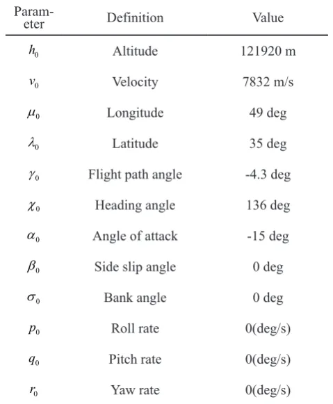
The initial flight conditions of the capsule have been presented in the Table 2
Table 1: Simulation parameters.
Value Definition
Param-eter
7985.5 59.7 503
2
59.7 7150.6 32.5
503 32.5 6456.4
kg m −
− −
− −
Moment of inertia matrix of the
capsule
I
N.m
1 sin( ) sin( )
125 250
2
1 sin( ) sin( ) 10
125 250
1 sin( ) sin( )
125 250
t t
t t
t t
π π
π π
π π
+ +
+ + ×
+ +
External disturbance matrix
d
0.2 I Uncertainties in
the Moment of inertia matrix
I∆
5000 N.m Maximum
controller output
umax
-5000 N.m Minimum
controller output
umin
0.05s Thruster model
time constant
T
Table 2: Initial conditions.
Param-eter Definition Value
0
h Altitude 121920 m
0
v Velocity 7832 m/s
0
µ Longitude 49 deg
0
λ Latitude 35 deg
0
γ Flight path angle -4.3 deg
0
χ Heading angle 136 deg
0
α Angle of attack -15 deg
0
β Side slip angle 0 deg
0
σ Bank angle 0 deg
0
p Roll rate 0(deg/s)
0
q Pitch rate 0(deg/s)
0
r Yaw rate 0(deg/s)
Table 3: Parameters of B.D.A controller
Parameter µ µ1, 2
ε
λ
εu0 Kp1=Kp2=Kp3 KI1=KI2=KI3 rˆu0( )
0 ρˆ( )
0101
5- 1- Simulation and control performance analysis of B.D.A controller
In this section, the simulation results and performance analysis of the B.D.A controller will be presented. The parameters of the B.D.A controller are summarized in Table 3.
The performance of the controller to track the guidance commands is shown in Figure 2. In this case, the tracking quality seems satisfactory and is in a great compliance with the desired values.
Figure 3 shows the guidance commands tracking errors. It shows that the maximum tracking error of the attack angle and side slip angle are less than 1 degree. The maximum tracking error of the bank angle is higher than 100 degrees. This is due to the inertia of the capsule when the guidance
commands change. The tracking errors can be reduced by augmenting the controller outputs constraints levels.
In Figure 4, the rates of angular velocity have been illustrated. It is clear that reference commands have been tracked properly by applying the proposed control algorithm.
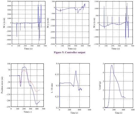
Figure 5 presents the controller outputs. It is obvious that the value of the controller’s outputs is less than the controller’s output constraints levels. Because of the stabilization of the re-entry capsule in pitch and yaw axis, a small controller output has been generated.
The load factor, landing accuracy, and L/D ratio are presented in Figure 6 that illustrates that the value of the load is less than 5g and landing accuracy is less than 500 m. Also, the L/D ratio is kept around 0.3.
0 100 200 300 400 500
-200 -100 0 100
Time (s)
σ
(de
g)
0 100 200 300 400 500
-30 -25 -20 -15 -10
Time (s)
α
(de
g)
0 100 200 300 400 500
-0.5 0 0.5 1
Time (s)
β
(de
g)
0 100 200 300 400 500
-200 -100 0 100 200
Time (s)
σ
e
rror (de
g)
0 100 200 300 400 500
-8 -6 -4 -2 0 2
Time (s)
α
e
rror (de
g)
0 100 200 300 400 500
-1 -0.5 0 0.5
Time (s)
β
e
rror (de
g)
Figure 2: Guidance commands tracking.
0 100 200 300 400 500
-200 -100 0 100
Time (s)
σ
(de
g)
0 100 200 300 400 500
-30 -25 -20 -15 -10
Time (s)
α
(de
g)
0 100 200 300 400 500
-0.5 0 0.5 1
Time (s)
β
(de
g)
0 100 200 300 400 500
-200 -100 0 100 200
Time (s)
σ
e
rror (de
g)
0 100 200 300 400 500
-8 -6 -4 -2 0 2
Time (s)
α
e
rror (de
g)
0 100 200 300 400 500
-1 -0.5 0 0.5
Time (s)
β
e
rror (de
g)
Figure 3: Guidance commands tracking error.
0 200 400 600
-100 -50 0 50
Time (s)
p (
de
g/
s)
0 200 400 600
-4 -2 0 2
Time (s)
q (
de
g/
s)
0 200 400 600
-50 0 50 100
Time (s)
p e
rr
or
(
de
g/
s)
0 200 400 600
-1 0 1 2 3 4
Time (s)
q e
rr
or
(
de
g/
s)
0 200 400 600
-20 -10 0 10 20
Time (s)
r e
rro
r (d
eg
/s
)
0 200 400 600
-20 -10 0 10 20
Time (s)
r
(
de
g/
s)
0 100 200 300 400 500 -5000
-4000 -3000 -2000 -1000 0 1000 2000 3000 4000 5000
Time (s)
M
x (
n.
m
)
0 100 200 300 400 500
-3000 -2500 -2000 -1500 -1000 -500 0 500
Time (s)
M
y (
n.
m
)
0 100 200 300 400 500
-1500 -1000 -500 0 500 1000 1500
Time (s)
M z
(n
.m
)
Figure 5: Controller output
0 100 200 300 400 500 -250
-200 -150 -100 -50 0 50 100
Time( s )
Pos
iti
on e
rror (m
)
0 200 400 600 0.2
0.25 0.3 0.35 0.4
Time (s)
L / D
ra
tio
0 200 400 600 0
1 2 3 4 5
Time (s)
Loa
d (g)
Figure 6: Landing accuracy (left), L/D ratio (center) and load on the vehicle (right).
In order to evaluate the performance of the B.D.A controller, the back-stepping dynamic inversion (B.D) controller has been designed to be used in the second control loop and the results will be compared with the proposed B.D.A controller.
5- 2- Simulation and control performance analysis of B.D controller
In this section, simulation of the B.D control algorithm will be performed based on a 6-DOF dynamical model of the capsule and the results analysis will be presented. The initial conditions are the same as conditions in the B.D.A controller which have been presented in the Table 2. The B.D controller parameters have been summarized in Table 4.
Figure 7 shows that the B.D controller performance is satisfactory as it tracks the guidance commands.
Figure 8 depicts reference angle tracking error by applying the B.D algorithm. The angle errors change according to variations of the reference guidance commands. These errors are less than 1 degree except in the cases where the reference guidance commands change abruptly due to the high inertia of the re-entry vehicle.
Reference angular rates tracking has been presented in Figure 9 which illustrates fine angular rate reference command tracking. Because of the coupling between re-entry capsule
axes, there is a close relation between roll rate and yaw rate of the re-entry capsule which causes yaw rate to change when roll rate varies.
The B.D controller outputs are shown in Figure 10. It shows that the controller outputs have exceeded controller output constraint (5000 N.m) in roll and yaw axes. In roll axis, the controller output is about -40000 N.m which is higher than the controller output constraint.
Table 4: Parameters of the B.D controller
Parameter Value Parameter Value
1
p
K 0.4 KI3 0.04
2
p
K 0.5 Kp21 5
3
p
K 0.3 Kp22 7
1
I
K 0.05 Kp23 4
2
I
103
0 200 400 600
-200 -100 0 100
Time (s)
σ
(de
g)
0 200 400 600
-30 -25 -20 -15 -10
Time (s)
α
(de
g)
0 200 400 600
-1 -0.5 0 0.5
Time (s)
β
(de
g)
0 200 400 600
-200 -100 0 100 200
Time (s)
σ
e
rro
r (d
eg
)
0 200 400 600
-8 -6 -4 -2 0 2
Time (s)
α
e
rro
r (d
eg
)
0 200 400 600
-0.5 0 0.5 1
Time (s)
β
e
rro
r (d
eg
)
Figure 7: Attitude angle tracking.
0 200 400 600
-200 -100 0 100
Time (s)
σ
(de
g)
0 200 400 600
-30 -25 -20 -15 -10
Time (s)
α
(de
g)
0 200 400 600
-1 -0.5 0 0.5
Time (s)
β
(de
g)
0 200 400 600
-200 -100 0 100 200
Time (s)
σ
e
rro
r (d
eg
)
0 200 400 600
-8 -6 -4 -2 0 2
Time (s)
α
e
rro
r (d
eg
)
0 200 400 600
-0.5 0 0.5 1
Time (s)
β
e
rro
r (d
eg
)
Figure 8: Attitude angle tracking error.
0 200 400 600
-100 -50 0 50
Time(s)
p (
de
g/
s)
0 200 400 600
-4 -2 0 2
Time(s)
q (
de
g/
s)
0 200 400 600
-20 -10 0 10 20
Time(s)
r (
de
g/
s)
0 200 400 600
-100 -50 0 50
Time (s)
p e
rr
or
(
de
g/
s)
0 200 400 600
-4 -2 0 2
Time (s)
q e
rr
or
(
de
g/
s)
0 200 400 600
-20 -10 0 10 20
Time (s)
r e
rro
r (d
eg
/s
)
Figure 9: Attitude angle rate tracking
0 100 200 300 400 500
-5 -4 -3 -2 -1 0 1 2
3x 10
4
Time (s)
M
x (
n.
m
)
0 100 200 300 400 500
-4000 -3500 -3000 -2500 -2000 -1500 -1000 -500 0 500 1000
Time (s)
M
y (
n.
m
)
0 100 200 300 400 500
-8000 -6000 -4000 -2000 0 2000 4000 6000 8000 10000 12000
Time (s)
Mz
(n
.m
)
According to the simulation results of the B.D.A and B.D controller, a comparison between B.D.A and B.D controllers can be summarized as follows:
1. Both B.D.A and B.D controllers provide a stable control system in the presence of the external disturbances and uncertainties in the moment of inertia matrix. The angle of attack and side slip angle errors are less than 1 degree.
2. The controller’s output in the B.D controller is greater than 40000 N.m in the roll axis while the B.D.A controller’s output is less than 5000 N.m in the same conditions.
3. The controller’s output in the B.D controller is greater than 8000 N.m in the yaw axis while the B.D.A controller’s output is less than 5000 N.m in the same conditions.
4. The B.D controller is more sensitive to the model uncertainties than the B.D.A controller. Hence, the B.D.A controller is more appropriate than the B.D controller in the phase of re-entry.
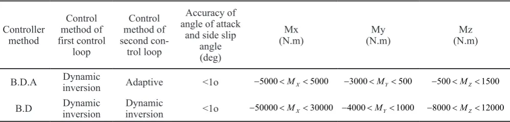
The results of comparison between the B.D and B.D.A controllers are summarized in Table 5.
According to Table 5, it is clear that the B.D.A controller is more effective than the B.D controller and generates lower controller’s output in the same conditions.
6- Conclusion
In this paper, a new attitude control algorithm, called B.D.A, has been designed based on backstepping dynamic inversion and adaptive control methods to control the attitude of a low L/D re-entry vehicle in the presence of the external disturbances, uncertainties in the moment of inertia, controller’s output constraints and the thruster’s model. In this method, the dynamic inversion algorithm has been designed to control the attitude angles using the kinematic equations of the vehicle. Then, an adaptive mechanism has been designed to control the attitude angular rates using the dynamical equations.
A single control variable bank angle has been considered to control the attitude of the re-entry capsule. The simulation results have shown that the B.D.A controller can provide a stable guidance command tracking. The proposed controller’s outputs are less than 5000 N.m. The B.D.A controller results have been compared with those of the B.D controller to evaluate the performance of the B.D.A controller. The simulation results have shown that the B.D controller is very sensitive to the model uncertainties and the external disturbances and it generates too high (higher than 40000 N.m) controller’s output while the B.D.A controller output is less than 5000 N.m in the same conditions. It means that,
in comparison with the B.D controller, the proposed B.D.A method is more effective to control the attitude of the re-entry capsule in the presence of the model uncertainties and the external disturbances.
Nomenclature
Symbols Definitions Symbols Definitions
h
AltitudeL
Lift forceV
VelocityD
Drag forceµ
LongitudeY
Side slipforce
λ
Latitudem
Capsule massγ
Flight pathangle
I
Moment of inertia matrix
χ
Headingangle
u
Controller outputα
Angle of attackR
E Radios of earthβ
Side slip angleΩ
E velocity of Angular earthσ
Bank angleT
mode time Thrusterconstant
p
Roll ratee
Tracking errorq
Pitch rated
disturbanceExternalr
Yaw rate∆
I
Uncertainty in moment
of inertia matrix
Ω
Vector of at-titude anglev
Desired thrusterinput
ω
Vector of at-titude anglerate
τ
Real torque of thruster Table 5: Comparison between the B.D and B.D.A controllers.
Controller method
Control method of first control
loop
Control method of second con-trol loop
Accuracy of angle of attack
and side slip angle (deg)
Mx
(N.m) (N.m)My (N.m)Mz
B.D.A inversionDynamic Adaptive <1o −5000<MX<5000 −3000<MY <500 −500<MZ <1500
105 References
[1] D. Isakeit, A. Wilson, P. Watillon, T. Leveugle, C. Cazaux, G. Bréard, The atmospheric reentry demonstrator, 1998. [2] T. Petsopoulos, F.J. Regan, J. Barlow, Moving-Mass
Roll Control System for Fixed-Trim Re-Entry Vehicle, Journal of Spacecraft and Rockets, 33(1) (1996) 54-60. [3] Z.R. Putnam, R.D. Braun, R.R. Rohrschneider, J.A. Dec,
Entry System Options for Human Return from the Moon and Mars, Journal of Spacecraft and Rockets, 44(1) (2007) 194-202.
[4] Y. Luo, A. Serrani, S. Yurkovich, M.W. Oppenheimer, D.B. Doman, Model-Predictive Dynamic Control Allocation Scheme for Reentry Vehicles, Journal of Guidance, Control, and Dynamics, 30(1) (2007) 100-113. [5] Z.-Q. Pu, R.-Y. Yuan, X.-M. Tan, J.-Q. Yi, An Integrated
Approach to Hypersonic Entry Attitude Control, International Journal of Automation and Computing, 11(1) (2014) 39-50.
[6] B. Tian, W. Fan, R. Su, Q. Zong, Real-Time Trajectory and Attitude Coordination Control for Reusable Launch Vehicle in Reentry Phase, IEEE Transactions on Industrial Electronics, 62(3) (2015) 1639-1650.
[7] D. Dirkx, E. Mooij, Continuous aerodynamic modelling of entry shapes, American Institute of Aeronautics and Astronautics (AIAA), 2011.
[8] Z. Prime, C. Doolan, B. Cazzolato, Longitudinal’L’adaptive control of a hypersonic re-entry experiment, in: AIAC15: 15th Australian International Aerospace Congress, Australian International Aerospace Congress, 2013, pp. 717.
[9] Y.-Z. Sheng, J. Geng, X.-D. Liu, L. Wang, Nonsingular finite-time second order sliding mode attitude control for reentry vehicle, International Journal of Control, Automation and Systems, 13(4) (2015) 853-866.
[10] F. Wang, Q. Zong, B. Tian, Adaptive Backstepping Finite Time Attitude Control of Reentry RLV with Input Constraint, Mathematical Problems in Engineering, 2014 (2014) 19.
[11] A. Cavallo, F. Ferrara, Atmospheric re-entry control for low lift/drag vehicles, Journal of Guidance, Control, and Dynamics, 19(1) (1996) 47-53.
[12] D.J. Leith, W.E. Leithead, Gain-Scheduled Control: Relaxing Slow Variation Requirements by Velocity-Based Design, Journal of Guidance, Control, and Dynamics, 23(6) (2000) 988-1000.
[13] S. Roy, A. Asif, Robust parametrically varying attitude controller designs for the X-33 vehicle, in: AIAA Guidance, Navigation, and Control Conference and Exhibit, American Institute of Aeronautics and Astronautics, 2000.
[14] D.-c. Xie, Z.-w. Wang, W.-h. Zhang, Attitude controller for reentry vehicles using state-dependent Riccati equation method, Journal of Central South University, 20(7) (2013) 1861-1867.
[15] X. Yunjun, X. Ming, V. Prakash, Nonlinear Stochastic Control Part II: Ascent Phase Control of Reusable Launch Vehicles, in: AIAA Guidance, Navigation, and Control Conference, American Institute of Aeronautics and Astronautics, 2009.
[16] R.R. da Costa, Q.P. Chu, J.A. Mulder, Re-entry Flight Controller Design Using Nonlinear Dynamic Inversion, Journal of Spacecraft and Rockets, 40(1) (2003) 64-71. [17] J. Georgie, J. Valasek, Evaluation of Longitudinal
Desired Dynamics for Dynamic-Inversion Controlled Generic Reentry Vehicles, Journal of Guidance, Control, and Dynamics, 26(5) (2003) 811-819.
[18] V. John, I. Daigoro, W. Donald, Robust dynamic inversion controller design and analysis for the X-38, in: AIAA Guidance, Navigation, and Control Conference and Exhibit, American Institute of Aeronautics and Astronautics, 2001.
[19] S. Juliana, Q. Chu, J. Mulder, T. Baten, Non-linear Dynamic Inversion versus Gain Schedulin, in: 56th International Astronautical Congress of the International Astronautical Federation, the International Academy of Astronautics, and the International Institute of Space Law, American Institute of Aeronautics and Astronautics, 2005.
[20] Y. Shtessel, C. Hall, M. Jackson, Reusable Launch Vehicle Control in Multiple-Time-Scale Sliding Modes, Journal of Guidance, Control, and Dynamics, 23(6) (2000) 1013-1020.
[21] J.-L. Chang, Robust dynamic output feedback second-order sliding mode controller for uncertain systems, International Journal of Control, Automation and Systems, 11(5) (2013) 878-884.
[22] G. Jie, S. Yongzhi, L. Xiangdong, Second-order time-varying sliding mode control for reentry vehicle, International Journal of Intelligent Computing and Cybernetics, 6(3) (2013) 272-295.
[23] X. Wu, S. Tang, J. Guo, Y. Zhang, Finite-Time Reentry Attitude Control Using Time-Varying Sliding Mode and Disturbance Observer, Mathematical Problems in Engineering, 2015 (2015) 19.
[24] Y.B. Shtessel, J.J. Zhu, D. Daniels, Reusable launch vehicle attitude control using a time-varying sliding mode control technique, in: System Theory, Proceedings of the Thirty-fourth Southeastern Symposium on, IEEE, 2002, pp. 81-85.
[25] J. Geng, Y. Sheng, X. Liu, Finite-time sliding mode attitude control for a reentry vehicle with blended aerodynamic surfaces and a reaction control system, Chinese Journal of Aeronautics, 27(4) (2014) 964-976. [26] C. Bai, C. Lian, Z. Ren, Y. Fan, P. Qi, Adaptive Tracking
Control of Hypersonic Re-entry Vehicle with Uncertain Parameters, in: Instrumentation, Measurement, Computer, Communication and Control (IMCCC), Third International Conference on, 2013, pp. 1594-1597. [27] Z. Shi, Y.f. Zhang, C.d. He, Adaptive robust control for
maneuvering reentry vehicle basing on backstepping, in: Control Conference (CCC), 33rd Chinese, 2014, pp. 2064-2068.
[28] F. Wang, Q. Zong, Q. Dong, Robust adaptive attitude control of reentry vehicle with input constraint and uncertainty, in: Control Conference (CCC), 34th Chinese, 2015, pp. 704-709.
Please cite this article using:
A. Mohseni, F. Fani Saberi, M. Mortazavi, Adaptive Attitude Controller of Reentry Vehicles Based on Back-stepping Dynamic Inversion Method, AUT J. Model. Simul. Eng., 50(1)(2018) 95-106.
DOI: 10.22060/miscj.2017.12907.5048
control of hypersonic vehicles in the presence of modeling uncertainties, in: American control conference, IEEE, 2009, pp. 3178-3183.
[30] F. Wang, C. Hua, Q. Zong, Attitude control of reusable launch vehicle in reentry phase with input constraint via robust adaptive backstepping control, International Journal of Adaptive Control and Signal Processing, 29(10) (2015) 1308-1327.
[31] Q. Zou, F. Wang, L. Zou, Q. Zong, Robust adaptive constrained backstepping flight controller design for re-entry reusable launch vehicle under input constraint, Advances in Mechanical Engineering, 7(9) (2015) 1687814015606308.
[32] L. Wang, Y. Sheng, X. Liu, A novel adaptive high-order sliding mode control based on integral sliding mode, International Journal of Control, Automation and Systems, 12(3) (2014) 459-472.
[33] Z. Wang, Z. Wu, Y. Du, Adaptive sliding mode
backstepping control for entry reusable launch vehicles based on nonlinear disturbance observer, Proceedings of the Institution of Mechanical Engineers, Part G: Journal of Aerospace Engineering, (2015) 0954410015586859. [34] P.N. Desai, B.A. Conway, Six-Degree-of-Freedom
Trajectory Optimization Using a Two-Timescale Collocation Architecture, Journal of Guidance, Control, and Dynamics, 31(5) (2008) 1308-1315.
[35] W.R. Van Soest, Q.P. Chu, J.A. Mulder, Combined Feedback Linearization and Constrained Model Predictive Control for Entry Flight, Journal of Guidance, Control, and Dynamics, 29(2) (2006) 427-434.
[36] Hagen, Modelling and controller design considering actuator dynamics, Narwik university college, 2006. [37] K. Hassan, Nonlinear Systems, Departement of