Ann. Geophys., 26, 3295–3316, 2008 www.ann-geophys.net/26/3295/2008/ © European Geosciences Union 2008
Annales
Geophysicae
Least-squares multi-spacecraft gradient calculation with automatic
error estimation
J. De Keyser
Belgian Institute for Space Aeronomy (BIRA-IASB), Ringlaan 3, 1180 Brussels, Belgium Received: 27 June 2008 – Accepted: 12 September 2008 – Published: 21 October 2008
Abstract. Multi-spacecraft missions allow the gradient of important physical quantities in the terrestrial environment to be determined. The gradient can be computed from four simultaneous measurements in a straightforward way, but this computation does not produce proper error estimates, making it hard to assess the meaningfulness of the result. Recently developed least-squares gradient computation tech-niques offer the possibility to obtain more precise results with all-inclusive error estimates, provided that information about the non-linearity of the space and time variations of the ob-served quantity is given. The present paper describes several heuristics for estimating these variations, thereby enabling a fully automatic computation of the gradient and the associ-ated error estimates. The performance of these heuristics is illustrated with synthetic data corresponding to 4- and 10-spacecraft configurations.
Keywords. Magnetospheric physics (Magnetospheric con-figuration and dynamics; Instruments and techniques)
1 Introduction
Computing gradients from in situ measurements is an es-sential element of multi-spacecraft missions, in particular the CLUSTER mission consisting of four identical space-craft flying in formation. The classical gradient computa-tion (CGC) technique exploits the fact that exactly four si-multaneous non-coplanar measurements are needed to deter-mine the three spatial gradient components (Harvey, 1998; Chanteur, 1998; Chanteur and Harvey, 1998; Robert et al., 1998a; Darrouzet et al., 2006). Although the basic idea is simple, such gradient computations are difficult in practice. A first set of problems has to do with the requirement of homogeneity: Computing the gradient makes sense only if Correspondence to: J. De Keyser
the true gradient does not deviate too much from the average gradient over the spacecraft configuration. A second set of problems is related to the measurement precision: gradients are differences of data values that differ only slightly, which inevitably leads to large relative errors on the results. This is true in particular when the spacecraft are closely spaced, which is often required by the homogeneity conditions. A third set of problems is due to imperfect knowledge of the ex-act place and time where the measurements are made, owing to uncertainties in the spacecraft positions, spacecraft clock synchronization errors, and the data acquisition time dura-tion. Finally, while it is possible to assess the uncertainty on the computed spatial gradient that results from the mea-surement errors, the instantaneous four-spacecraft calcula-tion provides no informacalcula-tion about the error that stems from the fact that the gradient in reality is not constant over the spacecraft tetrahedron.
Many of these difficulties can be succesfully addressed by least-squares gradient computation (LSGC), as recently de-scribed by De Keyser et al. (2007). The rationale is that, if the gradient remains constant over a given time interval (thus relaxing the requirement of simultaneity), the information content from a larger set of data points can be exploited for computing the gradient. An overdetermined problem is then obtained from which the space-time gradient can be com-puted in a weighted least-squares sense. The error made by approximating the field by a locally linear one (“approxima-tion error” or “curvature error”) is related to the distance of the measurement points from the point where the gradient is computed. The approximation error is expressed in terms of the homogeneity length and time scales. The total error on the data consists of this approximation error and the measure-ment error. The inverse of the total error is used as the weight of the measurement, so that only points close to the center of the homogeneity domain contribute to the solution. An error estimate on the gradient is obtained that accounts for both sources of error. Many data points are usually involved in the
3296 J. De Keyser: Gradient calculation with automatic error estimation
2 J. De Keyser: Gradient calculation with automatic error estimation
somewhat suppressed.
Gradient computations suffer badly from systematic errors on the data: They require properly intercalibrated data. How-ever, intercalibration is difficult as the instruments and their operating environments are never identical. Systematic gra-dient computations with ESA’s CLUSTER multi-spacecraft mission have been limited to magnetometer data (FGM in-strument, Balogh et al., 1997, 2001) with their high pre-cision and good calibration (Dunlop et al., 2001; Dunlop and Balogh, 2005; Vallat et al., 2005; Dunlop et al., 2006), and to electron density data derived from the plasma fre-quency (WHISPER instrument, D´ecr´eau et al., 1997, 2001; Trotignon et al., 2003) because of their absolute calibration (Darrouzet et al., 2006; De Keyser et al., 2007).
De Keyser et al. (2007) assume that the homogeneity length and time scales are given. While they point out that a suitable value can be chosen based on physical consider-ations, this may not always be easy to do in practice. They also take this scale factor to be constant over the analysis time interval, while the degree of curvature may change as the spacecraft traverse different regions of geospace. The goal of the present paper is to introduce heuristic techniques to estimate the homogeneity scales (and thus the approx-imation error) automatically. Armed with such estimates, this least-squares gradient computation with adaptive scales (LSGC-AS) will use an appropriately sized homogeneity do-main with the optimal set of data points, and the total error estimate on the computed gradient will be much more realis-tic.
Section 2 briefly reviews the least-squares gradient com-putation technique. We adopt standard linear algebra nota-tion: Bold lower-case symbols represent vectors, bold upper-case symbols are matrices, and all other symbols denote scalars. Section 3 introduces various ways for modelling the approximation error. Section 4 describes techniques for auto-matic estimation of the parameters in those descriptions. The techniques will be illustrated with synthetic data correspond-ing to 4- and 10-spacecraft configurations in Section 5. The paper ends with an evaluation of the proposed techniques.
2 Least-squares gradient computation
This section summarizes the least-squares technique devel-oped by De Keyser et al. (2007) for computing the gradient. We slightly generalize the description of the approximation error as this will turn out to be useful later on.
2.1 Problem formulation
Consider a scalar field f(x, t)that is sampled at positions and timesxi = [xi;yi;zi;ti], i = 1, . . . , N, relative to a given reference frame in 4-dimensional space-time. The measurementsfi have known random error variancesδfm2i and there are no systematic errors. The cross-correlations be-tween measurement errors at different points vanish. To illus-trate the idea, consider the 2-dimensional situation sketched
x1 x2
l2u2
l1u1
sc 3 sc2 sc1
[image:2.595.93.244.64.242.2]x0
Fig. 1. Illustration of least-squares gradient computation in a 2-dimensional setting. The algorithm uses data obtained in a set of points in space-time. In this example, the data are acquired by three spacecraft (red dots on the dotted spacecraft trajectories); the method can deal with any number of spacecraft. The approximation error in each data point grows with its distance fromx0, where the
gradient is computed. This distance is measured in a frame (l1u1,
l2u2) that may be rotated and scaled relative to the original frame.
Points on the ellipse with semi-axesl1andl2 are assigned a unit
distance. Points inside the ellipse (dark shaded area) correspond to smaller distances and therefore a smaller error. Points outside that ellipse (lightly shaded region) will have a larger error so that they are less relevant, thus reflecting the homogeneity condition. Points outside the shaded regions are ignored.
in Fig. 1. We want to compute the gradient atx0from mea-surements made by several spacecraft (sc1,sc2, . . .). The measurement pointsxi are indicated by the red dots. The fieldf can be locally approximated by a Taylor expansion around x0. With ∆x = x− x0 the relative position of a measurement point, and denoting the function value, the gradient, and the Hessian at x0 byf0, g0 = ∇xtf0, and H0=∇xt∇xt>f0, this expansion gives
f(x) =f0+∆x>g0+
1
2∆x>H0∆x+. . . (1) Truncating this expansion after the linear term defines the approximating functionfa(x) = f0+∆x>g0and the ap-proximation errorδfa(x) = 12∆x>H0∆x+. . .. Requiring the residuals to be zero,
ri=r(xi) =fa(xi)−fi= 0, (2)
leads to a system ofNequations (one for each measurement) forf0andg0. The number of unknowns,M, is5. System (2) is usually overdetermined (N M) so that it cannot be satisfied exactly, but it can be solved in a least-squares sense. Approximation (1) is valid in a region aroundx0that can be described by a hyperellipsoid in 4-dimensional space-time (the dark shaded ellipse in Fig. 1). Such an ellipsoid is uniquely specified by four mutually orthogonal unit vec-torsuk, which constitute the columns of a rotation matrix Fig. 1. Illustration of least-squares gradient computation in a 2-dimensional setting. The algorithm uses data obtained in a set of points in space-time. In this example, the data are acquired by three spacecraft (red dots on the dotted spacecraft trajectories); the method can deal with any number of spacecraft. The approximation error in each data point grows with its distance fromx0, where the gradient is computed. This distance is measured in a frame (l1u1, l2u2) that may be rotated and scaled relative to the original frame. Points on the ellipse with semi-axesl1andl2 are assigned a unit distance. Points inside the ellipse (dark shaded area) correspond to smaller distances and therefore a smaller error. Points outside that ellipse (lightly shaded region) will have a larger error so that they are less relevant, thus reflecting the homogeneity condition. Points outside the shaded regions are ignored.
calculation of an individual gradient, depending on the size of the homogeneity domain relative to the spacecraft sepa-rations and the sampling frequency; the uncertainty due to random measurement errors can therefore be somewhat sup-pressed.
Gradient computations suffer badly from systematic errors on the data: They require properly intercalibrated data. How-ever, intercalibration is difficult as the instruments and their operating environments are never identical. Systematic gra-dient computations with ESA’s CLUSTER multi-spacecraft mission have been limited to magnetometer data (FGM in-strument, Balogh et al., 1997, 2001) with their high pre-cision and good calibration (Dunlop et al., 2001; Dunlop and Balogh, 2005; Vallat et al., 2005; Dunlop et al., 2006), and to electron density data derived from the plasma fre-quency (WHISPER instrument, D´ecr´eau et al., 1997, 2001; Trotignon et al., 2003) because of their absolute calibration (Darrouzet et al., 2006; De Keyser et al., 2007).
De Keyser et al. (2007) assume that the homogeneity length and time scales are given. While they point out that a suitable value can be chosen based on physical consider-ations, this may not always be easy to do in practice. They also take this scale factor to be constant over the analysis time interval, while the degree of curvature may change as
the spacecraft traverse different regions of geospace. The goal of the present paper is to introduce heuristic techniques to estimate the homogeneity scales (and thus the approx-imation error) automatically. Armed with such estimates, this least-squares gradient computation with adaptive scales (LSGC-AS) will use an appropriately sized homogeneity do-main with the optimal set of data points, and the total error estimate on the computed gradient will be much more realis-tic.
Section 2 briefly reviews the least-squares gradient com-putation technique. We adopt standard linear algebra nota-tion: Bold lower-case symbols represent vectors, bold upper-case symbols are matrices, and all other symbols denote scalars. Section 3 introduces various ways for modelling the approximation error. Section 4 describes techniques for auto-matic estimation of the parameters in those descriptions. The techniques will be illustrated with synthetic data correspond-ing to 4- and 10-spacecraft configurations in Sect. 5. The paper ends with an evaluation of the proposed techniques.
2 Least-squares gradient computation
This section summarizes the least-squares technique devel-oped by De Keyser et al. (2007) for computing the gradient. We slightly generalize the description of the approximation error as this will turn out to be useful later on.
2.1 Problem formulation
Consider a scalar field f (x, t )that is sampled at positions and timesxi=[xi;yi;zi;ti],i=1, . . . , N, relative to a given reference frame in 4-dimensional space-time. The measure-mentsfi have known random error variancesδfm2i and there are no systematic errors. The cross-correlations between measurement errors at different points vanish. To illustrate the idea, consider the 2-dimensional situation sketched in Fig. 1. We want to compute the gradient atx0 from mea-surements made by several spacecraft (sc1,sc2, . . .). The measurement pointsxi are indicated by the red dots. The fieldf can be locally approximated by a Taylor expansion aroundx0. With1x=x−x0the relative position of a mea-surement point, and denoting the function value, the gradient, and the Hessian atx0byf0,g0=∇xtf0, andH0=∇xt∇xt>f0, this expansion gives
f (x)=f0+1x>g0+ 1 21x
>
H01x+. . . (1) Truncating this expansion after the linear term defines the approximating functionfa(x)=f0+1x>g0and the approx-imation error δfa(x)=211x>H01x+. . .. Requiring the residuals to be zero,
ri =r(xi)=fa(xi)−fi =0, (2) leads to a system ofNequations (one for each measurement) forf0andg0. The number of unknowns,M, is 5. System (2)
J. De Keyser: Gradient calculation with automatic error estimation 3297 is usually overdetermined (NM) so that it cannot be
satis-fied exactly, but it can be solved in a least-squares sense. Approximation (1) is valid in a region aroundx0that can be described by a hyperellipsoid in 4-dimensional space-time (the dark shaded ellipse in Fig. 1). Such an el-lipsoid is uniquely specified by four mutually orthogonal unit vectors uk, which constitute the columns of a rota-tion matrix U=[. . . ,uk, . . .], and by the four homogene-ity length and time scaleslk, which define a scaling matrix L=diag([. . . , lk, . . .])(this notation means: the diagonal ma-trix with thelk on the diagonal). Transforming the problem into a new reference frame by means ofx0=Px=(UL)−1x, the ellipsoid becomes a hypersphere. We will often use the euclidian norm in the new frame:
k1x0k2=1x>UL−2U>1x.
If the new frame involves only a rescaling and no rotation (U=I), this simply amounts to
k1x0k2=X k
(1xk lk
)2.
The dark shaded ellipse in Fig. 1 corresponds tok1x0k≤1. Assume that an estimate for the approximation errorδfa is known. How to obtain such an estimate will be the sub-ject of Sect. 3. At present, it suffices to remark that this error increases withk1x0k. The total error consists of the mea-surement and the approximation error,
δfi2=δfm2i +δfa2i;
these are the diagonal elements of the total error covariance matrixC2. For the sake of simplicity small-scale fluctuation errors are not considered here (see De Keyser et al., 2007). We also do not address spacecraft position or timing errors. 2.2 Problem solution
The gradient is computed in a weighted least-squares sense by first multiplying system (2) withC−1. IfC2is diagonal, this amounts to multiplying each equation withwi=1/δfi, the weight for thei-th equation. If C2 is not diagonal, a diagonalization has to be computed first, which we will try to avoid as this can be very compute-intensive. Solving the weighted overdetermined system
ri/δfi =0 (3)
is equivalent to minimizing the least-squares expression
χ2= N X
i=1 ri2
δfi2.
The choice of weights makes sure that measurements with a large total error do not contribute much to the solution. In particular, data outside the homogeneity domain have a large approximation error and do not add any significant informa-tion. To limit the amount of computational work, the set of
data points that are used is limited to those whose total error is less than a given factorσ (typically, σ=1000) times the smallest total error in the set of data points. If the measure-ment errors are all equal, the domain from which data points are accepted then is a large ellipsoid (the lightly shaded el-lipse in Fig. 1). The number of measurements,N, is therefore rather large, so thatNM.
Solving the weighted least-squares minimization problem is a classical application of the singular value decomposition. Withq=[f0;LU>g0]grouping the unknowns, the linear ap-proximation can be written as fa=Aq=[1,L−1U>1X>]q. The solution of the weighted overdetermined system (3) can be expressed as
q=(A>C−2A)−1A>C−2f =Mf. (4)
The solution is obtained by applying the linear operatorMto the dataf. The inverse of the symmetrized weighted system matrixA>C−2Ais computed by means of the singular value decomposition ofZ=C−1A(see De Keyser et al., 2007, for more details). Expression (4) indicates how measurement errorsδf produce an error on the result:
δq=Mδf,
with covariances C2q=MC2M>=(A>C−2A)−1. Small sin-gular values therefore imply strong error propagation. In par-ticular, zero singular values indicate that the measurements do not completely define the solution. The singular values offer a convenient generalization of the tetrahedron geomet-ric factors (size, elongation, and planarity) for 4-spacecraft configurations (Robert et al., 1998b). In general,C2
qis not di-agonal: The errors on different solution components are cor-related. Such correlations are often ignored, and one adopts [diag(C2
q)]1/2as the error margins.
The least-squares gradient method can be applied to vec-tor fields as well; the number of unknowns then isM=15. The cross-correlations between the errors on the gradients of the different field components must be taken into account when computing the error margins on the curl or the diver-gence of the vector field. The least-squares method can also handle constraints, e.g., when a vector field is divergence-free (De Keyser et al., 2007), in which caseM=14. Applied to the magnetic field, this leads to a new curlometer since
j=∇×B/µ0if there is no time dependence.
The method described here relies on an unconstrained approximation of the scalar or vector field f. If f is strictly positive, like for plasma densities or temperatures, the method should be applied to logf rather than tof itself.
3 Modelling the approximation error
We consider different descriptions of the approximation error δfa, depending on the desired level of detail.
3298 J. De Keyser: Gradient calculation with automatic error estimation
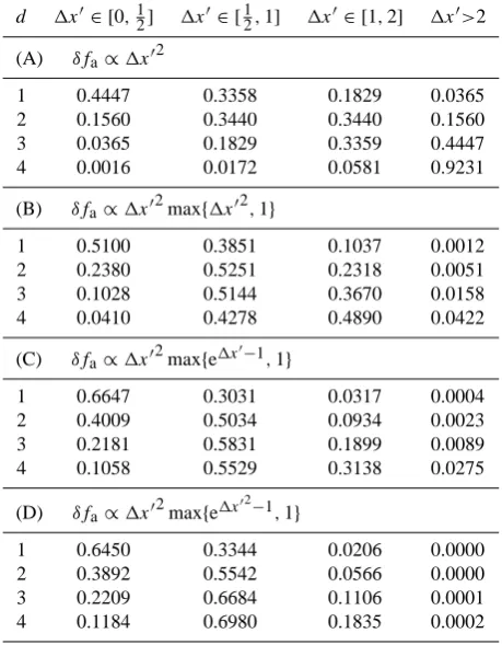
Table 1. Relative contributions of different regions in1x0-space to the least-squares solution for different approximation error models, assuming uniform coverage. See the text for an interpretation.
d 1x0∈ [0,12] 1x0∈ [1
2,1] 1x 0∈ [
1,2] 1x0>2
(A) δfa∝1x02
1 0.4447 0.3358 0.1829 0.0365
2 0.1560 0.3440 0.3440 0.1560
3 0.0365 0.1829 0.3359 0.4447
4 0.0016 0.0172 0.0581 0.9231
(B) δfa∝1x02max{1x02,1}
1 0.5100 0.3851 0.1037 0.0012
2 0.2380 0.5251 0.2318 0.0051
3 0.1028 0.5144 0.3670 0.0158
4 0.0410 0.4278 0.4890 0.0422
(C) δfa∝1x02max{e1x 0−1
,1}
1 0.6647 0.3031 0.0317 0.0004
2 0.4009 0.5034 0.0934 0.0023
3 0.2181 0.5831 0.1899 0.0089
4 0.1058 0.5529 0.3138 0.0275
(D) δfa∝1x02max{e1x 02
−1,1}
1 0.6450 0.3344 0.0206 0.0000
2 0.3892 0.5542 0.0566 0.0000
3 0.2209 0.6684 0.1106 0.0001
4 0.1184 0.6980 0.1835 0.0002
3.1 Weak and strong locality
It is clear that the approximation tends to degrade with dis-tance1x0=k1x0kaway fromx0, where the gradient has to be computed. By choosing the weights inversely propor-tional to the total error, the “(weak) locality principle” is sat-isfied: an individual point closer tox0contributes more to the least-squares solution than a point far away. De Keyser et al. (2007) use this principle to argue that the set of points included in the calculation can be limited (cf. theσ thresh-old that was introduced in Sect. 2). Upon closer inspection, however, it turns out that one must be very careful in draw-ing that conclusion. Let us assume that the approximation error can be modelled asδfa≤fc1x0p, wherefc is a scal-ing constant reflectscal-ing the approximation error at1x0=1. If the measurement errors are all the same, and equal tofc, the weights used in the least-squares problem are
w2i = 1 δfi2
= 1/f
2 c 1+1x02p.
The contributionζ of the set of points inside the homogene-ity domain to the computed solution can be quantified by summing the weights of these points, and comparing that to
the sum of the weights of all points. If the data points are distributed uniformly ind-dimensional space, and if this set of points is dense enough to use the continuous-distribution limit, it is found that
ζ = lim
R→∞Id(1)/Id(R),
where
Id(R)= Z R
0
w(ρ)Sd(ρ) dρ = Z R
0
dCdρd−1 1+ρ2p dρ,
in which the constantCd=Vd(ρ)/ρd, withVd(ρ)andSd(ρ) representing the volume and surface of a d-dimensional sphere with radiusρ, respectively. Whatever the value of p, there is always a dimensiond for whichId is unbounded forR→∞, so thatζ→0: The far-away points dominate the solution despite the fact that the weak locality principle is sat-isfied. Requiring that the solution is not dominated by the set of points outside the homogeneity domain, which we refer to as the “strong locality principle”, leads to 2p>d−1. For the space-time setting of the multi-spacecraft gradient problem (d≤4), this requirement is satisfied forp≤2. To be general for alld,δfamust increase at least exponentially with1x0: Only if the approximation error increases rapidly, the sum of the weights of far-away points decreases quickly enough to yield a finite contribution. Table 1 lists the relative con-tributions of the sets of points with different1x0-ranges in the uniform and continuous distribution limit, for four ap-proximation error bounds. Ford=4, a boundδfa∝1x02is problematic as more than 90% of the solution is contributed by points outside1x0>2. A higherpor an exponential error bound is needed to enforce strong locality; the table gives a few alternatives. The assumption of a uniform coverage of the homogeneity domain is often not realistic, as the num-ber of spacecraft is usually limited. As an alternative, con-sider the case where the data cover ad-dimensional cylinder whose cross-section has dimensions well below the homo-geneity scales, as for closely spaced spacecraft crossing a large structure. The contribution then is proportional toI1, giving the results listed in Table 1 ford=1, regardless of the actual dimensiond. For the quadratic approximation error bound, the contribution from points outside 1x0>2 is less than 4%, so that the situation is not that bad. Note that these assessments ofζ in different circumstances are rather crude since the approximation errors at different points are not sta-tistically independent. Summing or integrating the squared weights is therefore only indicative of the contribution of a particular set of points to the solution.
3.2 Homogeneity properties and the second-order term The approximation error is due to the second- and higher-order terms in the Taylor expansion (1):
δfa(1x0)=δfso(1x0)+δfho(1x0),
J. De Keyser: Gradient calculation with automatic error estimation 3299 whereδfso=O(1x02)is the second-order term,
correspond-ing to the term with the Hessian. It can be written as
δfsoi = 1 21xi
>
H01xi =fc d X
k=1 sk1x02ik
if the Hessian isH0=U3U>with3=diag(2fcsk/ lk2), that is, if the eigen-vectors of the Hessian are the homogene-ity directions, if its eigen-values λk determine the homo-geneity lengthslk=
√
2fc/|λk|and if the sense of curvature sk=signλkin each direction, withfcan a priori given scaling constant. The homogeneity properties therefore determine the second-order term in the Taylor approximation.
3.3 Description of the approximation error Because of the strong locality principle, we use
δfai =fc d X
k=1
sk1x02ik·max{η(1x
0)φ (1x0),1}
to express the approximation error, whereη(1x0)∈[−1,1]is bounded andφ (1x0)is a monotonically increasing function withφ (1)=1. Four approximation error models are consid-ered here: (A)φ≡1, (B) φ=1x02, (C)φ=e1x0−1, and (D) φ=e1x02−1. The actual behaviour of function η(1x0), and especially its sign, is not known. This limits our ability to estimate the variances. A simple estimate is
hδfa2ii ≤f 2 c(
d X
k=1
sk1x02ik)
2max{[φ (1x0 )]2,1}.
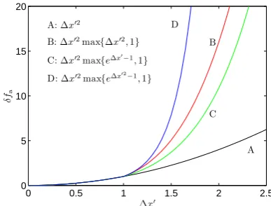
For1x0=1, the variance isδfa2≤fc2, in line with the defini-tion of the homogeneity lengths as the scales corresponding to an approximation errorfc. The above approximation er-ror estimate is correct for small1x0when the homogeneity properties are well estimated. The higher-order terms are de-scribed rather poorly, but points where those terms play a role do not contribute much to the solution anyway because of the strong locality principle. This can be appreciated by looking at the upper bounds given by the four approxima-tion error models. These are the four alternatives discussed in Table 1; they are illustrated for the one-dimensional case in Fig. 2. For1x0<1 the approximation error is quadratic in all four cases. For points that are farther away, the error grows more rapidly with alternatives B, C, and D, so that such points have substantially less weight. While model B initially grows faster than model C, the converse is true as 1x0→∞. Model D produces a very steep increase of the ap-proximation error, so that points beyond roughly1x0>1.7 do not count at all. In the sequel, model C has been adopted, as it offers the best compromise between guaranteeing strong lo-cality and allowing points outside1x0=1 to contribute some information to the solution.
The approximation errors at two pointsiandjare not in-dependent. Because of the lack of knowledge aboutη, we
J. De Keyser: Gradient calculation with automatic error estimation 5
3.3 Description of the approximation error
Because of the strong locality principle, we use
δfai=fc d
X
k=1
sk∆x0 2
ik·max{η(∆x0)φ(∆x0),1}
to express the approximation error, whereη(∆x0)∈[−1,1]
is bounded andφ(∆x0)is a monotonically increasing
func-tion withφ(1) = 1. Four approximation error models are considered here: (A)φ≡1, (B)φ= ∆x02
, (C)φ= e∆x0−1
, and (D) φ = e∆x02−1. The actual behaviour of function
η(∆x0), and especially its sign, is not known. This limits our ability to estimate the variances. A simple estimate is
hδfa2ii ≤fc2( d
X
k=1
sk∆x02ik)2max{[φ(∆x0)]2,1}.
For∆x0 = 1, the variance isδfa2≤fc2, in line with the def-inition of the homogeneity lengths as the scales correspond-ing to an approximation errorfc. The above approximation error estimate is correct for small∆x0when the
homogene-ity properties are well estimated. The higher-order terms are described rather poorly, but points where those terms play a role do not contribute much to the solution anyway because of the strong locality principle. This can be appreciated by looking at the upper bounds given by the four approxima-tion error models. These are the four alternatives discussed in Table 1; they are illustrated for the one-dimensional case in Fig. 2. For∆x0 <1the approximation error is quadratic in all four cases. For points that are farther away, the er-ror grows more rapidly with alternatives B, C, and D, so that such points have substantially less weight. While model B initially grows faster than model C, the converse is true as ∆x0 → ∞. Model D produces a very steep increase of the approximation error, so that points beyond roughly
∆x0 > 1.7do not count at all. In the sequel, model C has
been adopted, as it offers the best compromise between guar-anteeing strong locality and allowing points outside∆x0= 1
to contribute some information to the solution.
The approximation errors at two pointsiandjare not in-dependent. Because of the lack of knowledge aboutη, we can only assume that the covariances of the higher-order part of the solution vanish. In fact, as the higher-order terms rep-resent a residual error, typically with oscillatory behaviour, such correlations can indeed often be ignored. The covari-ances therefore are due to the second-order part alone:
hδfaiδfaji ≈fc2( d
X
k=1
sk∆x02ik)( d
X
k=1
sk∆x02jk).
In the particular situation where the signs sk are not known, an upper bound on the variances is given by
δfa2i ≈fc2∆x0 4
{[φ(∆x0)]2,1};
the covariances can only be taken zero. This simplified de-scription with a diagonal covariance matrixC2is computa-tionally much cheaper.
0 0.5 1 1.5 2 2.5
0 5 10 15 20 ∆x0 δf a
A: ∆x02
B: ∆x02max{∆x02,1}
C: ∆x02max{e∆x0−1
,1}
D: ∆x02max{e∆x02−1,1}
A B
[image:5.595.328.522.63.210.2]C D
Fig. 2. Behaviour of four different upper bounds for the approx-imation error. These four models adopt a quadratic behaviour for ∆x0 <1, but differ in the way in which they estimate the higher-order terms in the Taylor approximation for larger∆x0.
3.4 Role of error cross-correlations
Consider the following toy problem ford= 1withs1= +1, where the data points can be grouped in three sets: set I con-taining points well inside the homogeneity domain (∆x0 1), set II grouping points near the edge of the homogeneity domain (∆x0 ≈1), and set III containing points outside the
homogeneity domain (∆x0 =ξ >1). These sets containNa,
Nb, andNc points, respectively. For the sake of simplicity, considerδfmi≡fc. The covariance matrix then is
C2=fc2
I 0 0
0 I+E ξ2E
0 ξ2E [1+ξ4([φ(ξ)]2−1)]I+ξ4E
,
with cross-correlations due to the quadratic terms (Idenotes identity matrices,Erepresents matrices whose elements are all 1). With a scalingSC =fcdiag([. . .1. . .
√
2. . . s . . .]), wheres2= 1 +ξ4[φ(ξ)]2, one obtains
C2=SC>
I 0 0
0 12(I+E) √ξ2
2sE
0 √ξ2
2sE (1− ξ4 s2)I+ξ
4 s2E
SC
Ifφ is strictly increasing (as in models B, C, and D), the cross-correlations between points of sets II and III, and those among points of set III, are1/√2φ(ξ)and1/[φ(ξ)]2, which tend to zero asξ→ ∞, so that
C2≈SC>
I 0 0
0 12(I+E) 0
0 0 I
SC.
This indicates that only total error cross-correlations between points of set II matter: Those involving points of set I are neg-ligble since uncorrelated measurement errors dominate the total error there, while those involving points of set III are negligible since the second-order error is dwarfed by the un-correlated higher-order contributions there. The approximate eigen-values ofC2are the variances of set I,Natimesfc2, the Fig. 2. Behaviour of four different upper bounds for the approx-imation error. These four models adopt a quadratic behaviour for 1x0<1, but differ in the way in which they estimate the higher-order terms in the Taylor approximation for larger1x0.
can only assume that the covariances of the higher-order part of the solution vanish. In fact, as the higher-order terms rep-resent a residual error, typically with oscillatory behaviour, such correlations can indeed often be ignored. The covari-ances therefore are due to the second-order part alone:
hδfaiδfaji ≈fc2( d X
k=1
sk1x02ik)( d X
k=1
sk1x02j k).
In the particular situation where the signs sk are not known, an upper bound on the variances is given by
δfa2i ≈f 2 c1x
04{[
φ (1x0)]2,1};
the covariances can only be taken zero. This simplified de-scription with a diagonal covariance matrixC2is computa-tionally much cheaper.
3.4 Role of error cross-correlations
Consider the following toy problem ford=1 with s1=+1, where the data points can be grouped in three sets: set I con-taining points well inside the homogeneity domain (1x01), set II grouping points near the edge of the homogeneity do-main (1x0≈1), and set III containing points outside the ho-mogeneity domain (1x0=ξ >1). These sets containNa,Nb, andNcpoints, respectively. For the sake of simplicity, con-siderδfmi≡fc. The covariance matrix then is
C2=fc2
I 0 0
0 I+E ξ2E
0 ξ2E [1+ξ4([φ (ξ )]2−1)]I+ξ4E
,
with cross-correlations due to the quadratic terms (I denotes identity matrices,Erepresents matrices whose elements are
3300 J. De Keyser: Gradient calculation with automatic error estimation all 1). With a scaling SC=fcdiag([. . .1. . .
√
2. . . s . . .]), wheres2=1+ξ4[φ (ξ )]2, one obtains
C2=SC>
I 0 0
0 12(I+E) √ξ2 2sE 0 √ξ2
2sE (1− ξ4 s2)I+
ξ4 s2E
SC
If φ is strictly increasing (as in models B, C, and D), the cross-correlations between points of sets II and III, and those among points of set III, are 1/
√
2φ (ξ )and 1/[φ (ξ )]2, which tend to zero asξ→∞, so that
C2≈SC>
I 0 0
0 12(I+E) 0
0 0 I
SC.
This indicates that only total error cross-correlations between points of set II matter: Those involving points of set I are negligble since uncorrelated measurement errors dominate the total error there, while those involving points of set III are negligible since the second-order error is dwarfed by the uncorrelated higher-order contributions there. The approxi-mate eigen-values ofC2are the variances of set I,N
atimes fc2, the variances of set III,Nctimes(1+ξ4[φ (ξ )]2)fc2, and those of set II, which for the special form of the 12(I+E) diagonal block are known to be once(Nb−1)fc2andNb−1 timesfc2. The corresponding eigen-vectors indicate how the original set of equations is reordered into an equivalent set of equations that each represent a statistically independent piece of information. The equations for set I remain unaf-fected; the eigen-values indicate essentially the independent measurement error variances. The equations for set III are unaffected as well, corresponding to variances that reflect the higher-order errors. The equations for the points of set II, however, are linearly combined into a set ofNb−1 equations with an improved precision as the correlated second-order part of the error can be eliminated there, while there remains one equation with a much higher variance, which is equiva-lent to dropping that equation from the system.
Generalizing the conclusions of this toy problem to ar-bitrary distributions of data points, as well as to the multi-dimensional case, one finds that adding the cross-correlations helps to partially eliminate the effect of the approximation error in points near and beyond the edge of the homogeneity domain, but the contribution of those points is limited be-cause of the strong locality principle. Overall, including the correlation tends to reduce the error margin on the gradient a little, but it does not have a dramatic effect. Even rough estimates of the cross-correlations are therefore sufficient.
This has important practical consequences. Solving the weighted overdetermined problem requires inverting the to-tal error covariance matrix. This computationally very ex-pensive operation can be accelerated, for instance, by setting small correlations to zero in order to improve the sparsity of the matrix. An even more dramatic acceleration is obtained
by simply ignoring the cross-correlations, thus avoiding the inversion of the correlation matrix altogether.
4 Automatic determination of homogeneity parameters
The LSGC technique explained in Sect. 2 requires that an approximation error estimate is given. Section 3 showed how that error can be described in terms of the homogeneity directionsuk, the homogeneity scales lk, and the curvature sensessk. Applying the least-squares gradient method would be much easier if these parameters could be determined au-tomatically. It can intuitively be understood that this must somehow be possible: the residuals reflect the behaviour of the error, from which the parameter values can be extracted. We assume here that the orientationsuk in space-time are given: Most often, one direction is along the time axis, a sec-ond one is along the magnetic field direction, while there is no a priori homogeneity anisotropy perpendicular to the field. The set of parameter values that must be estimated there-fore is eitherS={lk}, orS={lk, sk}, depending on the desired level of detail. In all cases, approximation error model C has been used. It can sometimes be useful to adopt a more com-plicated choice for theuk. For instance, for convecting time-stationary structures, and knowing the convection speed (e.g. from plasma measurements), it can be advantageous to con-sider computing the gradients in the comoving frame defined by the specific choice of theuk as discussed by De Keyser et al. (2007, Appendix A2).
We will determine the parameter values by optimization: The least-squares gradient is computed for different sets of parameter values so as to minimize a functionF(S)that rep-resents the quality of a set. Different functionsF lead to different heuristic parameter estimation techniques.
4.1 Heuristics based onχ2
Ifqdenotes the gradient computed with parameter valuesS, thenAq are the observations that would have been made if the gradient were exact, andr=Aq−f are the residuals. It is a basic property ofχ2-statistics that
χ2=r>C−2r = N X
i=1 (ri
δfi
)2=N−M, (5)
the effective number of degrees of freedom. We can use this property to estimate the approximation error.
Starting with a set of parameter valuesS(n−1), the gradient is computed, as well as
χ2=X i
ri(n−1)2/δfi(n−1)2.
If this value matchesN−M, the specified variances did cor-respond to the observed variability. If this is not the case, something was wrong with the given error estimatesδfi(n−1).
J. De Keyser: Gradient calculation with automatic error estimation 3301 If the measurement errors are well-known, the approximation
error estimates must have been incorrect. Improved estimates δfi(n)and the corresponding residualsri(n)should satisfy N−M=Xri(n)2/δfi(n)2.
Changing the weights in the overdetermined problem only has a modest effect on its solution, so thatri(n)≈ri(n−1)and
δfi(n)2≈ χ 2
N−Mδf (n−1) i
2
=α(n)2δfi(n−1)2;
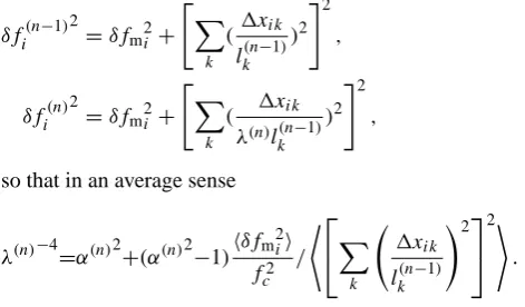
the factorα(n)should be used to rescale the total error esti-mates. To understand the consequences of this, assume that we are working with approximation error model A (second-order term only, without knowledge of curvature senses) and that the homogeneity directions are along the coordi-nate axes. Denoting the improved homogeneity lengths by lk(n)=λ(n)lk(n−1), the total error estimates are
δfi(n−1)2=δfm2i + "
X
k (1xik
lk(n−1) )2
#2 ,
δfi(n)2=δfm2i + "
X
k
( 1xik λ(n)l(n−1)
k )2
#2 ,
so that in an average sense
λ(n)−4=α(n)2+(α(n)2−1)hδfm 2 ii f2
c /
*
X
k
1xik
lk(n−1) !2
2
+
.
Such a solution exists only if the right hand side is positive. This condition is satisfied ifα(n)≥1, when the approximation error was underestimated. A solution also exists ifα(n)<1, but only if the measurement error is small compared to the approximation error: If the measurement errors dominate, rescaling the homogeneity lengths does not affect the residu-als very much. In the particular situation wherehδfm2iifc2, this amounts to rescaling the homogeneity lengths with a fac-torλ(n)=1/
√ α(n).
In conclusion: If the obtainedχ2 was too large, the ap-proximation error was underestimated and the homogeneity lengths must be decreased. Ifχ2was too small, the converse is true. Because of the simplifying assumptions made above, this adaptation process is an iterative one. As the process is repeated,α(n)→1. This amounts to minimizing
F=α2+ 1 α2 ≥2,
a technique that we call “localχ2optimization”. The min-imum of F is uniquely defined if the curvature lengths are lk=(limn→∞λ(n)·. . .·λ(1))lk(0)=λlk(0) with a direction-independent proportionality constant, so that minimizing F(lk(λ)) is a one-dimensional optimization problem. The
heuristic does not allow to estimate the individual homogene-ity lengths, nor the sense of curvature. Different initial ho-mogeneity scales in various directions can be specified; they are rescaled while keeping their relative proportions.
The value of α(n) and the corresponding scale λ(n) are some sort of mean value as the technique cannot distinguish the relative contributions from different directions. If one is dealing with gradients of one-dimensional structures (a rather common situation), the approximation error is due to one of theddimensions only, so that the actual rescaling fac-tor must be takend times larger. Even if there is no single dominant curvature direction, it is safe to do so. Also, as we work with three-standard-deviation error bounds rather than the one-standard-deviation bounds used in the defining property ofχ2, the corresponding factor must be added. Fi-nally, in order to give more emphasis to points where the ap-proximation error is small, we introduce an additional factor µ=2 to force the homogeneity lengths to be chosen a little bit smaller than they would otherwise. We therefore define α(n)2=9µ2d2 χ
2
N−M,
producing a rescaling that reflects the smallest spatial scale. If the number of available data,N, is not large, the statis-tical properties ofχ2 cannot be relied upon. This problem can be overcome by determining the correction not on the basis of an individual gradient computation, but for a set of gradient computations performed over a certain time inter-val. Doing so leads to proportionally larger values ofN,M, andN−M, so thatχ2-statistics do apply. The homogeneity scaleslk then remain constant throughout the time interval, so that this approach is useful only when the curvature prop-erties do not change significantly over that interval. We refer to this technique as “globalχ2optimization”.
[image:7.595.46.282.296.434.2]4.2 Heuristics based on the distribution of the residuals More detailed heuristics analyze the spatial distribution of the residuals to find thelkin each direction individually. Also the curvature signsskcan be determined.
Figure 3 sketches a typical distribution of the (non-weighted) residuals for the one-dimensional case. The mea-surement errors lead to non-zero values for k1xk close to zero. Farther away, the second-order terms lead to a quadratic behaviour. Still farther away, the higher-order terms dominate so that there is not necessarily an obvious systematic behaviour anymore. We can subtract the measure-ment errors and estimate the approximation errors
δfa2i ≈max{r 2
i −3hδfm2ii,0},
from which we try to recover the properties of the second-order errors.
A first possibility is to fit the approximation errors with a second-order expression of the form
|δfai| =fc1x 02
i
3302 J. De Keyser: Gradient calculation with automatic error estimation
J. De Keyser: Gradient calculation with automatic error estimation 7
so that in an average sense
λ(n)−4=α(n)2+ (α(n)2−1)hδfm 2 ii f2 c /h " X k
(∆xik
lk(n−1))
2
#2
i.
Such a solution exists only if the right hand side is positive. This condition is satisfied if α(n) ≥ 1, when the approxi-mation error was underestimated. A solution also exists if
α(n) <1, but only if the measurement error is small com-pared to the approximation error: If the measurement errors dominate, rescaling the homogeneity lengths does not affect the residuals very much. In the particular situation where hδfm2ii fc2, this amounts to rescaling the homogeneity lengths with a factorλ(n)= 1/√α(n).
In conclusion: If the obtainedχ2 was too large, the ap-proximation error was underestimated and the homogeneity lengths must be decreased. Ifχ2was too small, the converse is true. Because of the simplifying assumptions made above, this adaptation process is an iterative one. As the process is repeated,α(n)→1. This amounts to minimizing
F =α2+ 1 α2 ≥2,
a technique that we call localχ2 optimization. The min-imum of F is uniquely defined if the curvature lengths are lk = (limn→∞λ(n) · . . .· λ(1))l(0)k = λl
(0) k with a direction-independent proportionality constant, so that mini-mizingF(lk(λ))is a one-dimensional optimization problem. The heuristic does not allow to estimate the individual homo-geneity lengths, nor the sense of curvature. Different initial homogeneity scales in various directions can be specified; they are rescaled while keeping their relative proportions.
The value of α(n) and the corresponding scale λ(n) are some sort of mean value as the technique cannot distinguish the relative contributions from different directions. If one is dealing with gradients of one-dimensional structures (a rather common situation), the approximation error is due to one of theddimensions only, so that the actual rescaling fac-tor must be takendtimes larger. Even if there is no single dominant curvature direction, it is safe to do so. Also, as we work with three-standard-deviation error bounds rather than the one-standard-deviation bounds used in the defining property ofχ2, the corresponding factor must be added. Fi-nally, in order to give more emphasis to points where the ap-proximation error is small, we introduce an additional factor
µ= 2to force the homogeneity lengths to be chosen a little bit smaller than they would otherwise. We therefore define
α(n)2= 9µ2d2 χ
2
N−M,
producing a rescaling that reflects the smallest spatial scale. If the number of available data,N, is not large, the statis-tical properties of χ2 cannot be relied upon. This problem can be overcome by determining the correction not on the basis of an individual gradient computation, but for a set of gradient computations performed over a certain time inter-val. Doing so leads to proportionally larger values ofN,M,
0 1 2 3 4
0 1 2 3
k∆xk
|
r
[image:8.595.73.258.62.231.2]|
Fig. 3. Typical spatial distribution of the residuals in the one-dimensional case. The diamonds indicate the absolute values of the residuals. For smallk∆xk, the measurement errors dominate (measurement error bound: green line). At intermediate values, the order behaviour is evident (measurement error plus second-order term: blue curve). For largerk∆xk, higher-order terms play a role and may result in residuals whose upper bound can be higher or lower. The goal of solution adaptivity is to find the homogene-ity length scale (marked by the dashed vertical line), at which the transition of second-order to higher-order behaviour occurs.
andN−M, so thatχ2-statistics do apply. The homogeneity scaleslk then remain constant throughout the time interval, so that this approach is useful only when the curvature prop-erties do not change significantly over that interval. We refer to this technique asglobalχ2optimization.
4.2 Heuristics based on the distribution of the residuals
More detailed heuristics analyze the spatial distribution of the residuals to find thelkin each direction individually. Also the curvature signsskcan be determined.
Figure 3 sketches a typical distribution of the (non-weighted) residuals for the one-dimensional case. The mea-surement errors lead to non-zero values for k∆xk close to zero. Farther away, the second-order terms lead to a quadratic behaviour. Still farther away, the higher-order terms dominate so that there is not necessarily an obvious systematic behaviour anymore. We can subtract the measure-ment errors and estimate the approximation errors
δfa2i ≈max{r2i −3hδfm2ii,0},
from which we try to recover the properties of the second-order errors.
A first possibility is to fit the approximation errors with a second-order expression of the form
|δfai|=fc∆x0 2 i
to determine the parameter >0. This is an overdetermined problem. To eliminate the impact of the higher-order terms, weights w2
i = e−∆x
02
i/X2/∆x02
[image:8.595.353.503.63.217.2]i are associated with each Fig. 3. Typical spatial distribution of the residuals in the one-dimensional case. The diamonds indicate the absolute values of the residuals. For smallk1xk, the measurement errors dominate (measurement error bound: green line). At intermediate values, the order behaviour is evident (measurement error plus second-order term: blue curve). For largerk1xk, higher-order terms play a role and may result in residuals whose upper bound can be higher or lower. The goal of solution adaptivity is to find the homogene-ity length scale (marked by the dashed vertical line), at which the transition of second-order to higher-order behaviour occurs.
to determine the parameter>0. This is an overdetermined problem. To eliminate the impact of the higher-order terms, weightsw2i=e−1x02i/X2/1x02
i are associated with each equa-tion;X=3 is used here. The weighted least-squares solution is
= P
ie −1x02i/X2
|δfai|
fcPie−1x 02
i/X21x02
i .
We take the value 3to be an approximate upper bound for the approximation error. It is again possible to obtain a suit-able value corresponding to the smallest homogeneity scale by settingα(n)=3µd, similar to what was done forχ2 op-timization, implying a rescaling of the homogeneity lengths by a common factorλ(n)=1/
√
α(n) at each step. One can again define an optimization process that determines the ho-mogeneity scales that minimize
F=α2+ 1 α2 ≥2.
As α(n)→1 near the optimum, the homogeneity lengths lk=(limn→∞λ(n)·. . .·λ(1))lk(0)=λl(k0) have the desired val-ues. This “solution-adaptive technique with common rescal-ing” is similar to localχ2optimization.
A direction-dependent fit of the form |δfai| =fc
X
k
k1x02ik
x1 x2
l2u2
l1u1 sc3
sc2
sc1
x0
Fig. 4. If the spacecraft sample the homogeneity domain only par-tially, for instance only along homogeneity directionu1as sketched in this example, the residuals do not contain any information about the approximation error along the other directions so that the corre-sponding homogeneity lengths cannot be derived.
can be used to find the parameters k>0; this coincides with the previous technique if allk≡ are identical. The weighted least-squares solution can be formally written as
[k]= "
X
m
w2m1x02im1x02j m #−1"
X
m
w2m1x02km|δfak|/fc #
where the same weighting is used as before. One has to be careful to verify that all k≤0; if not, one has to explore a number of combinations in which one or more of thek are zero and the remaining values are computed from the above system of equations, and retain the solution that mini-mizes the weighted residuals. The effectively used values are taken asα(n)k =3µk>0, from which λk(n)=1/[αk(n)]1/2 and lk=(limk→∞λ(n)k ·. . .·λk(1))l(k0)=λklk(0).
It has been our experience that this multi-dimensional fit-ting procedure fails to work properly if the homogeneity do-main is only partially sampled. And this, unfortunately, is very often the case with data recorded by spacecraft that fly in formation along a common trajectory. Suppose that the spacecraft orbit is along one of the homogeneity direc-tions, as depicted in Fig. 4. If the homogeneity scales in the perpendicular directions happen to be much larger than the transverse spacecraft separations, the residuals do not contain much information about the approximation error in those di-rections, so that the corresponding homogeneity lengths can-not be properly estimated. This is can-not really a problem: As there are no data points in those directions, there is no need to evaluate the corresponding approximation errors, and so those homogeneity lengths are not needed. One only has to make sure that the heuristic technique is robust enough to handle such circumstances.
The strategy adopted here is to guide the direction-dependent heuristic by the direction-indirection-dependent one. First
J. De Keyser: Gradient calculation with automatic error estimation 3303 obtain αmax=1/λ2min from the common rescaling method,
corresponding to the minimum scale length in any direction. Then apply the direction-dependent technique. In each step we obtain theα(n)k values. Definingαˆk=αmax/Akwith Ak=α(nk −1)·. . .·α
(1) k ,
we set the effective direction-dependent rescaling factors to
logα(n)effk =logαˆk+max{logL2·erf √
πlog(α(n)k /αˆk) 2 logL2 ,0} whereL>1 is a given constant. This restrictsαeff(n)k to the in-terval[ ˆαk/L2,αˆk]if it was outside, while keepingαeff(n)k≈αk(n) inside that interval. This choice guarantees that
1 L2 ≤
αeff(n)kAk
αmax
≤1 and thus 1≤ l (n) k
λminl(k0) ≤L.
This choice therefore makes sure that the homogeneity lengths all lie in a bounded interval above the minimum length as determined by common rescaling. This makes this “solution-adaptive technique with direction-dependent rescaling” very robust, while at the same time allowing some adaptivity. The constantLcan be freely chosen, but it should not be too large to avoid ill-defined values when the homo-geneity domain is not well covered. The choiceL=10 has been adopted here, which is sufficient to capture the effects of direction-dependent homogeneity properties. The target function that is minimized in the direction-dependent case is
F= d X
k=1 αk2+ 1
α2k ≥2,
under the constraints discussed above.
Yet another way to improve the well-posedness of the direction-dependent adaptation process is to limit the number of unknown homogeneity scales by introducing constraints. For instance, one might require the spatial homogeneity lengths to be all equal. This is done by taking equal reference lengthsl(x0)=ly(0)=lz(0) and by forcingλx=λy=λz, while the homogeneity time is determined by a reference timelt(0)and a rescaling factorλt. The corresponding direction-dependent technique then becomes a two-dimensional optimization pro-cess, which is also computationally easier to solve.
The “solution-adaptive technique with direction-dependent rescaling and curvature” goes one step further: from the signs of the (non-weighted) residuals r=f−Aq
one can infer the curvature signssk. In this case, too, it can be useful to set constraints on the set of homogeneity scales; introducing constraints on the curvature signs, however, is of little practical use. The curvature sign in a particular direction is deemed to be zero if the corresponding homogeneity length is large: in such directions the curvature error is small. As explained in Sect. 3.3, knowing the signs allows a more precise evaluation of the approximation error.
It also allows the cross-correlations on the data used in the overdetermined system to be estimated, although we do not exploit that in order limit computation time.
4.3 Homogeneity parameters from a second-order fit An alternative approach would be to compute both a first-and a second-order fit, first-and use the difference between both as an error estimate. Computing a second-order fit is, how-ever, usually not feasible. A full quadratic fit implies many unknowns: M=15 for a scalar field (function value, gradi-ent, and symmetric hessian matrix) andM=45 for a vector field. In a simplified version where the homogeneity direc-tions are good approximadirec-tions of the eigen-vectors of the hessian, the hessian off-diagonals vanish, so that M=9 or M=27 for a scalar or a vector field. In either case, there usually is not enough information available to determine all these unknowns because the homogeneity domain is not fully covered by the sampling points.
4.4 Optimization procedure
The heuristic techniques described above rely on minimizing target function F, a multi-dimensional optimization prob-lem. The optimization algorithm used here is the classical Broyden, Fletcher, Goldfarb, and Shanno (BFGS) method with numerical derivatives. This algorithm progressively evolves from a steepest descent method to a quasi-Newton method. Starting from an initial guess and an estimate of the target function gradient at that point (obtained by numerical differentiation), a line search is performed to find the (ap-proximate) minimum in that direction. The line search iter-atively uses an interpolating parabola to approach that min-imum. This procedure is repeated, but at each step the tar-get function gradient is used to improve an estimate of the HessianHF of the target function near the minimum, from
which the next search direction is computed. Rather than storing the Hessian, one stores its Cholesky factorLF(where
HF=LF>LF); the BFGS algorithm relies on a specific
up-date and downup-date of the Cholesky factor that is computa-tionally efficient.
Given the algorithm to compute the least-squares gradi-ent and the choices made therein (such as the selection of data points to be used), the target functionF, while having a smooth overall behaviour as a function of its arguments, is not necessarily smooth locally. This behaviour manifests itself when solving the optimization problem with high preci-sion: The optimization might get trapped in a local minimum close to the global minimum. To avoid this, we let BFGS op-timization be followed by a comparison of the BFGS solution with the target function values in a set of nearby alternatives in all directions. If a lower value is found, BFGS is used to improve that solution even further.
We formally describe F as being a function of logα=−2 logl or logαk=−2 loglk. We solve each
3304 J. De Keyser: Gradient calculation with automatic error estimation optimization problem until the solution updates become
smaller than a specified precision of 10−6. This implies that the values ofl or lk are determined with a relative error of 0.1%, which is more than adequate for our purpose.
The globalχ2optimization heuristic requires solving one optimization problem in just a single variable. On one hand, the evaluation of the target function is pretty expensive, as it consists of computing the gradients at all points for the current values of the homogeneity lengths to evaluateα. On the other hand, for a one-dimensional search space the BFGS technique reduces to a line search, so that only a limited num-ber of evaluations is needed.
For the localχ2technique, an optimization problem must be solved at each point where the gradient is to be computed. Each optimization problem is one-dimensional, with a tar-get function that involves computing one gradient, which is fairly easy.
The solution-adaptive technique with common rescaling is similar to localχ2optimization: Only the definition ofαis different.
The solution-adaptive technique with direction-dependent rescaling is more expensive, in that there are nowd or 3d parameters at each point, the homogeneity scales for the scalar and vector cases, respectively. (The number of pa-rameters is less when constraints on the homogeneity scales are being used.) The heuristic benefits from the computa-tional efficiency of BFGS for such multi-dimensional prob-lems. We perform the optimization in three steps. First, the common rescaling problem is solved. The multi-dimensional direction-dependent problem is then solved with the BFGS algorithm, while forcing the homogeneity scales in a band within a factor L=
√
10 above the direction-independent minimum length. Finally, this solution is used as the start-ing guess for solvstart-ing the direction-dependent problem over again, now with L=10. Note that choosing a larger value ofLwould require solving the optimization problem up to a (much) larger precision; as explained before, the valueL=10 is quite sufficient for our purposes.
If the signs are to be computed as well, this would increase the dimension of the search space even more. However, be-cause of their discrete nature, they are treated differently: First, a solution is computed corresponding to the common rescaling case. This solution is then improved by solving the directional-dependent rescaling case for unknown signs. As the result is pretty close to the final solution, the signs can be determined at this point. Finally, a more detailed cal-culation of the homogeneity lengths is carried out with the given signs, first withL=
√
10 and then with L=10. This procedure circumvents the need to solve a mixed continuous-discrete multi-dimensional optimization problem.
The optimization processes needed for iteratively estab-lishing the homogeneity parameters are computationally ex-pensive: The gradients at each point have to be computed a number of times. One way to accelerate this optimization would be to use the solution obtained in the previous point as
a starting guess for the optimization at the next point. This is advantageous mostly in cases where the gradients are com-puted with a rather high time resolution, since then the homo-geneity lengths do not change much from point to point. For testing purposes, however, we have not followed this strategy here: By keeping the computation at each point independent from that in the other points it is easier to evaluate the cor-rectness and the efficiency of the optimization processes.
5 Algorithm performance
In this section we illustrate the performance of LSGC-AS with the error estimation heuristics proposed above.
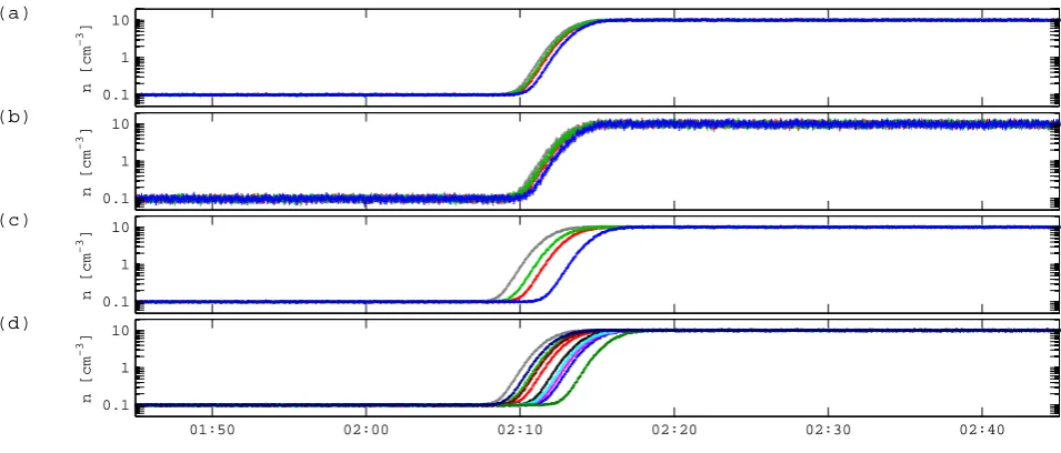
5.1 Gradient of a scalar field: a planar transition layer In a first series of tests we consider a planar interface in a scalar field, e.g. plasma density (see Fig. 5). The interface has its normal direction alongx and is characterized by a smooth transition profile of the form
n(x)=nl
1+erf(x/D)
2 +nr
1−erf(x/D)
2 .
The two asymptotic densities are chosen as nl=0.1 cm−3 and nr=10 cm−3 and the characteristic half-thickness is D=100 km. Synthetic data have been produced for multi-spacecraft constellations, in which the multi-spacecraft fly through the interface along parallel straight lines from the left (x<0) to the right (x>0) with a constant speedvx=1 km s−1, while moving along the y-direction with vy=0.5 km s−1; there is no motion alongz. The synthetic data sample the structure at 5 s resolution. Note that there is only a single direction of varying curvature in this example.
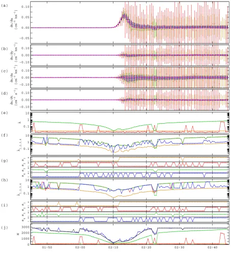
We first consider the case of a 4-spacecraft constellation that is about 150 km wide, on the order of the layer thick-ness. The spacecraft therefore cross the boundary with de-lays that are less than the crossing duration (Fig. 5a). The relative errors on the data have a normal distribution with a three-standard-deviation range of 5% (constant relative er-ror). The x-, y-, z-, and t-axes are taken to be the homogene-ity directions. The reference homogenehomogene-ity lengths have been chosen isotropic in space, withl(x0)=ly(0)=l(z0)=1000 km, and the reference homogeneity time scale islt(0)=600 s. The ap-proximation error scaling factor isfc=1 cm−3. The gradi-ents were computed with a selection limitσ=1000.
The least-squares gradient of (the logarithm of) the den-sity has been computed every 30 s. Figure 6a–d shows the space-time gradient components obtained with diffent heuristic techniques for estimating the approximation er-ror. Each of these techniques provides the gradient with a different total error estimate. The figure plots the re-sults for global χ2 optimization (orange), local χ2 opti-mization (red), solution-adaptive common rescaling (green), direction-dependent rescaling with curvature while requiring