International Doctorate School in Information and
Communication Technologies
DISI - University of Trento
O
PTIMIZATION
M
ODULO
T
HEORIES
WITH
L
INEAR
R
ATIONAL
C
OSTS
Silvia Tomasi
Advisor:
Prof. Roberto Sebastiani
Universit`a degli Studi di Trento
In the contexts of automated reasoning (AR) and formal verification (FV),
important decision problems are effectively encoded into Satisfiability Modulo
Theories (SMT). In the last decade efficient SMT solvers have been developed
for several theories of practical interest (e.g., linear arithmetic, arrays,
bit-vectors). Surprisingly, little work has been done to extend SMT to deal with
op-timization problems; in particular, concerning the development of SMT solvers
able to produce solutions which minimize cost functions over arithmetical
vari-ables (we are aware of only one very-recent work [60]).
In the work described in this thesis we start filling this gap. We present and
discuss two general procedures for leveraging SMT to handle the minimization
of linear rational cost functions, combining SMT with standard minimization
techniques. We have implemented the procedures within the MathSAT SMT
solver. Due to the absence of competitors in AR and FV, we have
experimen-tally evaluated our implementation against state-of-the-art tools for the domain
oflinear generalized disjunctive programming (LGDP), which is closest in spirit to our domain, and a very-recent SMT-based optimizer [60]. Our benchmark
set consists of problems which have been previously proposed for our
competi-tors. The results show that our tool is very competitive, and often outperforms
these tools (especially LGDP ones) on their problems, clearly demonstrating
the potential of the approach.
Stochastic Local-Search (SLS) procedures are sometimes very competitive
tools which are commonly based on the lazy approach (it combines a Conflict-Driven-Clause-Learning (CDCL) SAT solver with theory-specific decision
pro-cedures, called T-Solvers). We first introduce a general procedure for
inte-grating a SLS solver of the WalkSAT family with a T-Solver. Then we present a
group of techniques aimed at improving the synergy between these two
compo-nents. Finally we implement all these techniques into a novel SLS-based SMT
solver for the theory of linear arithmetic over the rationals, and perform an
empirical evaluation on satisfiable instances. Although the results are
encour-aging, we concluded that the efficiency of proposed SLS-based SMT techniques
is still far from being comparable to that of standard SMT solvers.
Keywords
1 Introduction 1 1.1 Main Contribution: Optimization Modulo Theories with Linear
Rational Costs . . . 1
1.2 A Secondary Contribution: Stochastic Local Search for SMT . . 3
1.3 Structure of the Thesis . . . 5
1.4 Previous Publication . . . 7
I Background and State of the Art 9 2 Background 11 2.1 Propositional Satisfiability . . . 12
2.1.1 Conflict-Driven Clause Learning SAT Solvers . . . 13
2.1.2 Sthocastic Local Search for SAT . . . 17
2.2 Satisfiability Modulo Theories . . . 22
2.2.1 The Satisfiability Modulo Theories Problem . . . 22
2.2.2 Theory Solvers . . . 26
2.2.3 Lazy SMT Solvers . . . 29
2.2.4 Lazy SMT for Combinations of Theories . . . 34
2.3 Linear Generalized Disjunctive Programming . . . 38
2.3.1 Linear Programming . . . 38
2.3.4 Linear Generalized Disjunctive Programming . . . 42
3 State of the Art and Related Work 47 3.1 State of the Art . . . 47
3.1.1 Optimization in SAT: MaxSAT and Pseudo-Boolean Op-timization . . . 47
3.1.2 SMT with Pseudo-Boolean Costs and MaxSMT . . . 51
3.2 Other Forms of Optimization in SMT . . . 54
3.3 A Very-Recent OMT(LA(Q)) Tool . . . 55
II Novel Contributions 57 4 Optimization in SMT(LA(Q)∪T) 59 4.1 Basic Definitions and Notation . . . 59
4.2 Theoretical Results . . . 61
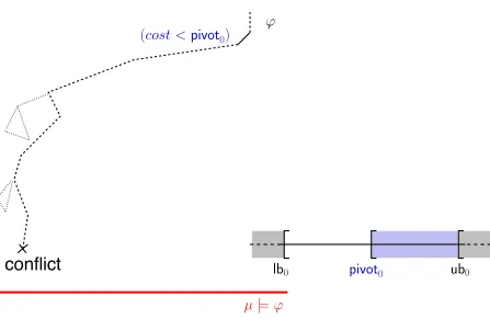
4.2.1 OMT(LA(Q)∪T) wrt. other Optimization Problems . 69 5 Procedures for OMT(LA(Q)) and OMT(LA(Q)∪T) 73 5.1 An Offline Schema for OMT(LA(Q)) . . . 74
5.1.1 Handling strict inequalities . . . 77
5.1.2 Discussion. . . 78
5.2 An Inline Schema for OMT(LA(Q)) . . . 80
5.3 Extensions to OMT(LA(Q)∪T ) . . . 85
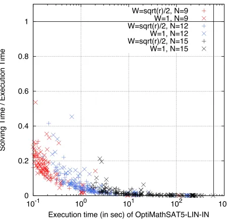
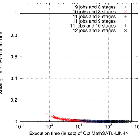
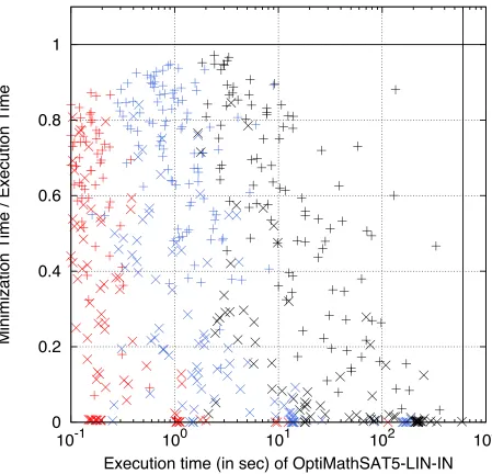
6 Experimental Evaluation for OMT(LA(Q)) 87 6.1 Encodings. . . 89
6.2 Comparison on LGDP Problems . . . 91
6.2.1 The strip-packing problem. . . 91
6.3 Comparison on SMT-LIB Problems . . . 112
6.3.1 Discussion . . . 114
6.4 Comparison on SAL Problems . . . 119
6.4.1 Discussion . . . 120
6.5 Comparison on Pseudo-Boolean SMT Problems . . . 124
6.5.1 Discussion . . . 124
6.6 Comparison on SYMBA Problems . . . 129
6.6.1 Discussion . . . 130
7 Stochastic Local Search in SMT 141 7.1 Intuition . . . 142
7.2 A basic WalkSMT procedure . . . 144
7.3 Efficient T-solvers for local search. . . 145
7.4 Enhancements to the basic WalkSMT procedure . . . 146
7.4.1 Preprocessing . . . 146
7.4.2 Single and Multiple Learning . . . 148
7.4.3 Filterings . . . 150
8 Experimental evaluation for WalkSMT 153 8.1 Environment and Settings . . . 153
8.2 WALKSMT on SMT-LIB Instances . . . 155
8.3 WALKSMT on Random Instances . . . 166
8.4 Discussion . . . 169
9 Conclusions and Future Research Directions 171
Introduction
In the contexts of automated reasoning (AR) and formal verification (FV), im-portant decision problems are effectively encoded into and solved as Satisfi-ability Modulo Theories (SMT) problems. In the last decade efficient SMT solvers have been developed, that combine the power of modern conflict-driven clause-learning (CDCL) SAT solvers with dedicated decision procedures (T
-Solvers) for several first-order theories of practical interest like, e.g., those of equality with uninterpreted functions (EUF), of linear arithmetic over the ra-tionals (LA(Q)) or the integers (LA(Z)), of arrays (AR), of bit-vectors (BV), and their combinations. (See [79, 18] for an overview.)
1.1
Main Contribution: Optimization Modulo Theories with
Linear Rational Costs
Many SMT-encodable problems of interest, however, may require also the ca-pability of finding models that are optimal wrt. some cost function over con-tinuous arithmetical variables.1 E.g., in (SMT-based) planning with resources [94] a plan for achieving a certain goal must be found which not only
ful-1Although we refer to quantifier-free formulas, as it is frequent practice in SAT and SMT, with a little abuse of
terminology we often call “Boolean variables” the propositional atoms and we call “variables” the free constants
fills some resource constraints (e.g. on time, gasoline consumption, ...) but that also minimizes the usage of some of such resources; in SMT-based model checking with timed or hybrid systems (e.g. [11, 10]) you may want to find executions which minimize some parameter (e.g. elapsed time), or which min-imize/maximize the value of some constant parameter (e.g., a clock timeout value) while fulfilling/violating some property (e.g., minimize the closure time interval of a rail-crossing while preserving safety). This also involves, as par-ticular subcases, problems which are traditionally addressed as disjunctive pro-gramming (DP) [13] or linear generalized disjunctive programming (LGDP) [75, 78], or as SAT/SMT with Pseudo-Boolean (PB) constraints and (weighted partial) MaxSAT/SMT problems [76, 59, 70, 31, 32]. Notice that the two latter problems can be easily encoded into each other.
Surprisingly, little work has been done so far to extend SMT to deal with op-timization problems [70, 31, 80, 40, 32, 63, 60]. In particular, to the best of our knowledge, most such works aim at minimizing cost functions over Boolean variables (i.e., SMT with PB cost functions or MaxSMT), whilst very little ef-fort has been put into extending SMT solvers for producing solutions which minimize cost functions over arithmetical variables (we are aware of only one very-recent work [60]). Notice that the former optimization problem can be easily encoded into the latter, but not vice versa.
In this thesis we try to fill this gap producing the following contributions:
• We define theOptimization ModuloLA(Q)∪T (OMT(LA(Q)∪T)) prob-lem which extends SMT(LA(Q) ∪ T ) for finding models which mini-mize some LA(Q)cost variable —T being some (possibly empty) stably-infinite theory s.t. T and LA(Q)are signature-disjoint.
a black-box; the second, called inline, is more sophisticate and efficient, but it requires modifying the code of the SMT solver. This distinction is important, since the source code of most SMT solvers is not publicly available.
• We have implemented these procedures within the MATHSAT5 SMT solver [33]. Due to the absence of competitors from AR and FV we have exper-imentally evaluated our implementation against state-of-the-art tools for the domain of LGDP, which is closest in spirit to our domain, on sets of problems which have been previously proposed as benchmarks for the lat-ter tools. Notice that LGDP is limited to plain LA(Q), so that, e.g., it cannot handle combination of theories like LA(Q)∪ T. As a last-minute addendum to this work, we also compared our implementation with the very-recent SMT-based tool presented in [60] on the authors own bench-marks problems. The results show that our tool is very competitive, and often outperforms these tools (especially LGDP ones) on their problems, clearly demonstrating the potential of the approach.
1.2
A Secondary Contribution: Stochastic Local Search for
SMT
to wonder whether SLS can be exploited successfully also inside SMT tools, both solvers and optimizers. As side work, in this thesis we start investigating this issue.
Remarkably, CDCL and SLS SAT solvers are very different in the way they perform Boolean search. CDCL SAT solvers reason on partial truth assign-ments, which are updated in a stack-based manner. Moreover, they intensively use techniques like Boolean constraint-propagation (BCP), conflict-directed backtracking (backjumping) and learning, which are heavily exploited in the lazy-SMT paradigm and allow for very-efficient SMT optimization techniques like early pruning, theory-propagation, theory-driven backjumping and learn-ing(see [79, 20]). SLS SAT solvers, instead, reason on total truth assignments, which are updated by swapping the phase of single literals according to some mixed greedy/stochastic strategy. Moreover, they typically do not use BCP, backjumping and learning. Therefore, the problem of an effective integration of a T -solver with a SLS SAT solver is not a straightforward variant of the stan-dard integration with a CDCL solver in lazy SMT. Moreover, the stanstan-dard SMT optimization techniques mentioned above cannot be applied in a straightforward way.
In order to cope with these problems, we present the following contributions:
• We present a novel and general architecture for integrating aT-Solverwith a Boolean SLS solver, which is inspired by the idea of “partially-invisible” SAT formulas.
• We analyze the differences between the interaction of a T-solver with a CDCL-based and a SLS-based SAT solver, and we introduce and discuss a group of optimization techniques aimed at improving the synergy between an SLS solver and theT-solver.
SLS solvers with the LA(Q)-solver of MATHSAT [30].
• We provide an extensive experimental evaluation of our implementation. In particular, we evaluate the effects of the various optimization tech-niques, also comparing them against MATHSAT, on two groups of sat-isfiable instances: industrial problems coming from the SMT-LIB and randomly-generated unstructured problems. The results show that:
1. the enhanced techniques drastically improve the performances of the basic version,
2. the improved techniques drastically improve the performances of the basic version but WALKSMT cannot beat MATHSAT4.
Although the results are encouraging, we concluded that the efficiency of pro-posed SLS-based SMT techniques is still far from being comparable to that of standard SMT solvers.
1.3
Structure of the Thesis
This thesis is divided in two parts.
Part I provides the necessary background knowledge and terminology, and a survey of the literature on the topic of optimization in SAT and SMT.
procedures which underlies lazy SMT solvers, its main enhanced tech-niques, relevant features of decision procedures for SMT, and methods for theory combination. Finally, (§2.3) we introduce LGDP and its solu-tion approaches after recalling linear programming, mixed integer linear programming and disjunctive programming which inspired it and whose techniques are exploited by it.
Chapter 3 summarizes the state of the art and related work of optimization problems in the context of SAT and SMT. First, (§4) we describe optimiza-tion problems and procedures for solving them available in the literature of SAT (such as MaxSAT and Pseudo-Boolean Optimization) and SMT. In the context of SMT, we consider SMT with Pseudo-Boolean Costs and MaxSMT [70, 31, 6, 32]. Second, (§3.2) we report on other forms of optimization in SMT, such as the problem of finding minimum-cost as-signments [40] and the “ILP Modulo Theories” framework [63]. Finally, (§3.3) we introduce a very-recent SMT-based tool for optimization, called SYMBA [60].
Part II is dedicated to the description of the novel contributions of this thesis. Chapter 4 introduces the problem addressed in this thesis. First, (§4.1) we provide the definition of the Optimization Modulo Theory (OMT) prob-lem and the theoretical foundations of the procedures for solving OMT, where the background theory isLA(Q)∪T. Then, (§4.2.1) we show how the OMT(LA(Q) ∪ T) problem captures many interesting optimization problems described in the Part I.
Chapter 6 reports on an extensive experimental evaluation carried out for eval-uating the implementation of the proposed procedures (we call it OPTI-MATHSAT) against a LGDP tool, called GAMS. We consider different encodings (§6.1) and kind of benchmarks: (§6.2) LGDP problems (e.g. strip-packing and job-shop), (§6.3) SMT-LIB formulas augmented with cost functions, (§6.4) formulas obtained by using the SAL Model Checker on bounded verification problems, and (§6.5) Pseudo-Boolean SMT prob-lems. As last-minute comparison, (§6.6) we evaluate OPTIMATHSAT against the recently-proposed tool SYMBA [60].
Chapter 7 describes a novel and general architecture for integrating a theory specific solver forLA(Q)with a based SAT solver resulting in a SLS-based SMT solver, called WALKSMT. First, we present the main intuition (§7.1), a basic architecture (§7.2). Then, (§7.3) we describe the most im-portant features for efficient theory-specific decision procedures for SLS. Finally, (§7.4) we propose several enhanced techniques.
Chapter 8 presents the experimental evaluation conduced for evaluating the performance of WALKSMT and its enhancements. After introducing the experimental evaluation (§8.1), we report on experiments on SMT-LIB for-mulas and random generated problems (§8.2 and §8.3 respectively).
Chapter 9 briefly concludes the thesis and highlights directions for future work.
1.4
Previous Publication
Part I and Chapters 4, 5 and 7:
• Roberto Sebastiani and Silvia Tomasi. Optimization in SMT with LA(Q)
Cost Functions. In Proceedings of IJCAR 2012, the 6th International Joint Conference on Automated Reasoning. Manchester, UK, 2012. [80].
• Roberto Sebastiani and Silvia Tomasi. Optimization Modulo Theories with Linear Rational Costs. Submitted to ACM Transactions on Computational Logic – TOCL [81].
Chapters 7 and 8:
• Silvia Tomasi. Stochastic Local Search for SMT. Technical Report. DISI-10-060, DISI, University of Trento. [87]
• Alberto Griggio, Roberto Sebastiani and Silvia Tomasi. Stochastic Local Search for SMT: a Preliminary Report. In Proceedings of SMT 2009, the 7th International Workshop on Satisfiability Modulo Theories. Montreal, Canada, 2009. [47]
• Alberto Griggio, Quoc Sang Phan, Roberto Sebastiani and Silvia Tomasi Stochastic Local Search for SMT: Combining Theory Solvers with Walk-SAT. In Proceedings of FroCoS 2011, the 8th International Symposium
Background
In this chapter we provide the background concepts and terminology of Propo-sitional Satisfiability (SAT) (§2.1), Satisfiability Modulo Theories (SMT) (§2.2) and Linear Generalized Disjunctive Programming (LGDP) (§2.3).
Notation2.1. We introduce a uniform notation which shall be used both in this chapter and in the rest of the thesis. We use boldface lowercase lettersa,y for arrays and boldface uppercase lettersA,Y for matrices, standard lowercase let-ters a, y for single rational variables/constants or indices and standard uppercase lettersA, Y for Boolean atoms and index sets; we use the first five letters in the various forms a, ...e, ... A, ...E, to denote constant values, the last five v, ...z,
... V, ...Z to denote variables, and the letters i, j, k, I, J, K for indexes and
in-dex sets respectively, pedices .j denote the j-th element of an array or matrix, whilst apices.ij are just indexes, being part of the name of the element. We use lowercase Greek letters ϕ,φ,ψ, µ,η for denoting formulas and uppercase ones
Φ,Ψ for denoting sets of formulas.
Disclaimer. The material presented in §2.1 is standard in SAT and it is mostly taken from [79] (and in part from [65]) for§2.1.1 and from [52, 51, 53, 88] for
2.1
Propositional Satisfiability
Given A = {A1, A2, . . .} a non-empty set of primitive propositions, the lan-guage of propositional logic is the least set of formulas containing A and the primitive constants ⊤ and ⊥ (“true” and “false” respectively) and closed un-der the set of standard propositional connectives {¬,∧,∨,→,↔}. We call a propositional atom every primitive proposition in A, and apropositional literal every propositional atom (positive literal) or its negation (negative literal). We implicitly remove double negations: e.g., if l is the negative literal ¬Ai, by ¬l we mean Ai rather than ¬¬Ai.
A propositional formula is inconjunctive normal form(CNF), if it is written as a conjunction of disjunctions of literals: !i"jlij. Each disjunction of literals
"
j lij is called a clause. Aunit clauseis a clause with only one literal.
Given a propositional formula ϕ, we call a truth assignmentµ for ϕa func-tion mapping truth values{true,false}to propositional atoms ofϕ. With a little abuse of notation, we represent µ indifferently as a set of literals {l1, . . . , ln}, with the intended meaning that a positive [resp. negative] literal Ai means that Aiis assigned to true [resp. false], or as aconjunctionof literalsl1∧. . .∧ln; thus, e.g., we may say “li ∈ µ” or “µ1 ⊆ µ2” (i.e. µ2 extends µ1 and µ1 subsumes µ2), but also “¬µ” meaning the clause “¬l1 ∨. . .∨ ¬ln”.
A truth assignmentµsatisfiesϕ, writtenµ |= ϕ, if and only ifϕis true under that truth assignment. (µ is called model for ϕ). A truth assignment is called total if it assigns a value to all atoms in ϕ, partial otherwise. We say that ϕ is satisfiableif and only if there exists at least one model for it. Two formulas ϕ1 and ϕ2 are called equi-satisfiable if and only if there exists µ1 s.t. µ1 |= ϕ1 if and only if there existsµ2 s.t. µ2 |= ϕ2.
this is the case. The following sections shall describe modern SAT solvers based on two different search approaches:
Systematic Search, which traverses the search space of a problem instance in a systematic manner. This guarantees that eventually a solution is found or no solution exists.
Local Search, which inspects the search space of a problem instance by iter-atively moving from one search space position to a neighboring one on the basis of local knowledge only. This kind of algorithms are typically incomplete since there is no guarantee that eventually an existing solution is found.
2.1.1 Conflict-Driven Clause Learning SAT Solvers
Most modern SAT solvers are based on systematic search and are inspired by the well-known Davis-Putnam-Logemann-Loveland (DPLL) procedure [38]. These solvers take advantage of smart non-recursive implementation and very efficient data structures to handle Boolean formulas and assignments, and can be grouped into two families:
conflict-driven SAT solvers: the search process is guided by the analysis of the conflicts at every branch which fails [65];
look-ahead SAT solvers: the search process is built on top of a look-ahead procedure which calculates the reduction effect of the selection of each variable in a set [50].
Algorithm 1Conflict-Driven Clause Learning SAT Solver Require: ⟨ϕ, µ⟩
1: ifpreprocess(ϕ, µ) = CONFLICT then
2: return UNSAT 3: end if
4: loop
5: decide next branch(ϕ, µ)
6: loop
7: res←boolean constraint propagation(ϕ, µ)
8: ifres =SATthen
9: return SAT
10: else ifres=CONFLICTthen
11: blevel←analyze conflict(ϕ, µ)
12: ifblevel= 0then
13: return UNSAT
14: else
15: backtrack(blevel,ϕ, µ)
16: end if
17: else
18: break
19: end if
20: end loop
21: end loop
in a stack-based manner. It performs aPreprocessingstep in lines 1-3. The core part of the algorithm is given in the outer loop in lines 4-21, which alternates four main phases: Decision, Boolean Constraint Propagation (BCP), Conflict Analysis andBackjumping and Learning.
Preprocessing preprocess(ϕ, µ)rewrites the input formulaϕinto a simpler and equi-satisfiable formula updatingµaccordingly; if the resulting formula is unsatisfiable, then it returns UNSAT.
given pairs of clauses, detecting and dropping subsumed clauses.
Decision decide next branch(ϕ, µ) selects an unassigned literall from the pre-processedϕaccording to some heuristic function, and adds it to the assign-ment µ. The literal l is called decision literal end the number of decision literals in µafter this operation is calleddecision level ofl.
Modern CDCL solvers compute a score at the end of each branch privileg-ing variables that occurs in recently-learned clauses.
Boolean Constraint Propagation boolean constraint propagation(ϕ, µ) itera-tively deduces literals l deriving from the current assignment, and updates ϕ and µaccordingly; this step is repeated until one of the following facts happens:
• µsatisfies ϕand the procedure ends returning SAT;
• µfalsifies some clause ψ ofϕ (conflicting clause) and the procedures backtracks;
• no more literals can be deduced, so that the inner loop ends and a new decision is performed.
BCP is based on the iterative application ofunit propagation: if all but one literals in a clause ψ are false, then the lonely unassigned literall is added to µ, all negative occurrences of l in other clauses are declared false and all clauses with positive occurrences of l are declared satisfied. State-of-art SAT solver benefits of extremely efficient implementations of BMC (based on the two-watched-literal scheme [96]) and also other forms of deductions and formula simplification, e.g. on-line equivalence reasoning and variable and clause elimination.
level, that is, the literal corresponding to the nth decision and the literals derived by unit-propagation after that decision are labelled with n; each non-decision literal l inµis also labelled by a link to the clauseψl causing its unit-propagation (called the antecedent clause of l). When a clause ψ is falsified by the current assignment (in this case we say that a conflict occurs and ψ is the conflicting clause) a conflict clause ψ′ is computed from ψ such that ψ′ contains only one literal lu which has been assigned at the last decision level. ψ′ is computed starting from ψ′ = ψ by iter-atively resolving ψ′ with the antecedent clause ψl of some literal l in ψ′ (typically the last-assigned literal in ψ′), until some stop criterion is met. Some example follows: in the 1st-UIP Scheme the last-assigned literal in ψ′ is always picked and the process stops as soon as ψ′ contains only one literalluassigned at the last decision level; in thelast-UIP Scheme, lumust be the last decision literal;
Backjumping and Learning If the computedblevelis equal to 0, then the pro-cedure returns UNSATsince a conflict exists even without branching. Oth-erwise,backtrack(blevel,ϕ, µ)adds theblocking clause¬η toϕ(learning) and backtracks up to blevel (backjumping), popping out of µ all literals whose decision level is greater than blevel, and updating ϕ and µ accord-ingly.
Other techniques often implemented in CDCL-based SAT solvers are:
search restarts causing the procedure to restart itself. Notice that previously-learned clauses are not deleted;
Modern CDCL SAT solvers often provide two important features:
stack-based incremental interface, by which it is possible to push/pop (the blocks of clauses corresponding to) sub-formulas φi into a stack of
formu-las Φ =def {φ1, ...,φk}, and check incrementally the satisfiability of !ki=1φi.
The interface maintains the status of the search from one call to the other, also storing learned clauses. Consequently, when invoked on Φ the solver can reuse a clauseC which was learned during a previous call on some Φ′
if C was derived only from clauses which are still in Φ (provided C was not discharged in the meantime); in particular, if Φ′ ⊆ Φ, then the solver can reuse all clauses learned while solvingΦ′.
unsatisfiable-core extraction is the capability of CDCL SAT solvers, when Φ
is found unsatisfiable, to return the subset of formulas in Φ which caused the unsatisfiability ofΦ. Notice that such subset is not unique, and it is not necessarily minimal1.
2.1.2 Sthocastic Local Search for SAT
Local searchapproach [53, 52] (see definition in§2.3) is widely used for solving hard combinatorial search problems. The idea is to examine the search space of a problem instance starting at some position and then iteratively moving from the present position to a neighboring one, where each location has a relatively small number of neighbors and moves are determined by decisions based on local knowledge only. When LS algorithms make use of randomized choices during both the initialization and the search process or of additional memory for storing historical information, they are calledStochastic Local search (SLS) algorithms. SLS algorithms are typically incomplete, however, in case of prob-lems which are known to be solvable by nature or of optimization probprob-lems
where the goal is to find a solution of sufficiently high quality, the ability to prove that no solution exists is not relevant.
SLS algorithms make use of an evaluation function for guiding the search towards solutions. It maps search positions onto real numbers the solutions of a given problem instance correspond to global minima of this function. However they can get stuck in local minima (i.e. positions having no improving neigh-bors) and plateau regions (i.e. regions not containing high-quality solutions) of the search space causing the premature stagnation of the search. There are many mechanisms for avoiding this, for example random restart which reini-tializes the search if after a fixed number of steps (cutoff time) no solution has been found, or diversification steps such as random moves.
Generally SLS algorithm are often advantageous if the knowledge of the problem domain is rather limited and when relatively good solutions are re-quired in a limited time, SLS algorithms returns the best solution found so far whereas systematic algorithms usually cannot provide approximated solutions.
SLS algorithms have been successfully applied to the solution of many NP-complete decision problems, including SAT. Typically SLS algorithms for SAT work with a CNF input formula (namely ϕ) and share a common high-level schema:
• initialization of the search by generating an initial truth assignment µ for ϕ (typically at random);
• iteratively selection of one (or more) Boolean atom Ai ofϕ which is then flipped within the current truth assignmentµ.
Algorithm 2Schema of WalkSAT Algorithms Require: ⟨ϕ,MAX TRIES,MAX FLIPS⟩
1: fori= 1toMAX TRIESdo
2: µ←initial truth assignment(ϕ)
3: forj = 1toMAX FLIPS do
4: if(µ|=ϕ)then
5: return SAT
6: else
7: c←choose unsatisfied clause(ϕ)
8: µ←next truth assignment(ϕ, c)
9: end if
10: end for
11: end for
12: return UNKNOWN
use random restarts.
In this section we focus on WalkSAT, a popular family of SLS-based SAT algorithms [53, 52].
WalkSAT Algorithms
The schema of WalkSAT algorithms is shown in Algorithm 2. It takes as input a CNF formulaϕand two integer constants MAX TRIES and MAX FLIPS. Initially, initial truth assignment selects a complete truth assignment µ for the variables ofϕ (line 2) according to some heuristic criterion (e.g. uniformly at random). The search proceeds iteratively by selecting and flipping a variable in µusing a two-stage process:
1. choose unsatisfied clause selects a currently-unsatisfied clause c ∈ ϕ ac-cording to some heuristic criterion (e.g. uniformly at random) (line 7).
(line 8).
The procedure terminates when a solution is found (line 5) or after MAX TRIES sequences of MAX FLIPS variable flips without finding a model forϕ(line 12).
Over the last ten years, several variants of the basic WalkSAT algorithm have been proposed [83, 66, 88], which differ mainly for the different heuristics used for the functions described above —in particular on the degree of greediness and randomness and in the criteria used for selecting the variable to flip in c within
next truth assignment. One of the best performing WalkSAT-based algorithm for SAT seems to be Adaptive Novelty+ [51, 88]. It adopts the Novelty+’s vari-able selection heuristic, and it adjusts its degree of greediness according to the search progress. Novelty+ deterministically chooses the variable to be flipped from cdepending on two mechanisms:
score function which computes the difference in the total number of satisfied clauses a flip would cause,
memory which stores variable’s age, i.e. the number of search steps performed since a variable was last flipped.
The variable selection heuristic works as follows:
1. if the variable with the highest score does not have minimal age among the variables in c, then it is selected;
2. otherwise, it is selected with a probability 1− p, where p is a parameter (callednoise setting). While in the remaining casesp, the variable is picked uniformly at random (i.e. random walk).
diversificationandintensificationrespectively). Search stagnation is detected if no progress in finding a solution has been observed over the last θ×m search steps, where m is the number of clauses of ϕ and θ is an input parameter. For this reason, each timepchanges, the current score function value is stored. Dur-ing the search the noise settDur-ing is increased byp = p+(1−p)×φand decreased by p = p−p ×φ/2, where φ is an input parameter; the asymmetry is due to the fact that detecting search stagnation is computationally more expensive than detecting search progress.
Trimming Variable Selection and Literal Commitment Strategy.
A few attempts have been made in order to enhance SLS algorithms with tech-niques borrowed from CDCL solvers (e.g. [23, 12]). This thesis focuses on the work of Belov and Stachniak [23], who propose two techniques that exploit the search history to improve the variable selection process of the classic SLS procedures for SAT. They modify the WalkSAT schema by adding a database (DB) that represents a set of constraints that help to guide the search process. It consists in:
• a partial truth assignment η that records assignments made by the local search heuristic (namely η ⊆ µ);
• a set of clausesψ obtained by storing selected unsatisfied-clauses (see line 7 of Algorithm 2).
The proposed techniques are inspired to clause learning and unit propagation, which are widely used by modern SAT solvers working with partial truth as-signments (see§2.1.1):
checks the satisfiability of ψ∧η′ by unit propagation, whereη′ is obtained from η by adding the (flipped) truth assignment of v under µ. If it is un-satisfiable, the variable v cannot be flipped. When all variables cause a conflict, the database is reset (i.e. η is set to∅) so that any variable inccan be chosen by the local search heuristic. Notice that, once the truth value of a variable has been flipped, η is updated accordingly and the clause cis added to the database.
Literal commitment strategy aims at exploiting the power of unit propaga-tion inside SLS procedures that naturally work with total truth assignments rather than partial ones. It iteratively deduces literals l in ψ deriving from η (i.e. ψ∧η |= l) and updates the current total truth assignmentµ accord-ingly during a single search step.
2.2
Satisfiability Modulo Theories
In this section we illustrate the background on the Satisfiability Modulo The-ories (SMT) problem. We first recall theoretical concepts and terminology in order to provide the definition of the problem; then we present the main ap-proaches for solving it.
2.2.1 The Satisfiability Modulo Theories Problem
In what follows we recall some basic notions and terminology about first-order theories. We assume the standard syntax and semantics of first-order logic with equality as defined, e.g., in [91].
Ift1, . . . , tn areΣ-terms and P is a predicate symbol, thenP(t1, . . . , tn)is aΣ -atom. Ift1 andt2are twoΣ-terms, then theΣ-atomt1 = t2is called aΣ-equality and ¬(t1 = t2) (also written as l ̸= r) is called a Σ-disequality. A Σ-formula ϕ is built in the usual way out of the universal and existential quantifiers ∀,∃, the Boolean connectives ∧,¬ and Σ-atoms. We apply the standard Boolean abbreviations, e.g. “φ1 ∨ φ2” for “¬(¬φ1 ∧ ¬φ2)”, “φ1 → φ2” for “¬(φ1 ∧
¬φ2)”, “⊤” [resp. “⊥” ] for the true [resp. false] constant. A Σ-literal is either aΣ-atom or its negation (i.e. a positive literal or anegative literal). By notation, we use the capital letters Ai and Bi to represent Boolean atoms, and the Greek letters α,β to representΣ-atoms. AΣ-formula isquantifier-free if it does not contain quantifiers, and a sentence if it has no free variables. As for propositional formulas, a quantifier-free formula is in CNF if it is written as a conjunction of disjunctions of literals.
We writeΓ |= φ to denote that the formulaφ is a logical consequence of the (possibly infinite) setΓ of formulas. AΣ-theory is a set of first-order sentences with signatureΣ. We consider theories which are first-order theories with equal-ity. This means the equality symbol = is a predefined predicate and it is always interpreted as the identity on the underlying domain (so it will not be included in any signature Σ considered in this thesis). As a result, = is interpreted as a relation which is reflexive, symmetric, transitive, and it is also a congruence.
We call the Σ-structure I a model of a Σ-theory T if I satisfies every sen-tence inT . A Σ-formula is satisfiablein T (or T-satisfiable) if it is satisfiable in a model of T. A Σ-formula is valid in T (or T-valid) if it is satisfiable in all models of T. We write Γ |=T φ to intend T ∪ Γ |= φ. Two Σ-formulae φ and ψ are T -equisatisfiable if and only if φ is T-satisfiable if and only if ψ is
T-satisfiable.
Satisfiability Modulo Theory(SMT(T) for short) is the problem of deciding theT-satisfiability ofΣ-formulas, for some background theoryT2.
In this thesis we only consider quantifier-freeΣ-formulas on someΣ-theory
T (notice that the variables are implicitly existentially quantified). Therefore, when we refer to SMT(T)we mean the satisfiability problem inT of quantifier-free formulas. As it is frequent practice in SAT and SMT, with a little abuse of terminology we refer to predicates of arity zero (i.e. propositional atoms) as Boolean variables, uninterpreted constants asTheory variables(orT-variables) and free constantsxiin quantifier-free linear arithmetic atoms (e.g.,(3x1−2x2+ x3 ≤3)) as variables.
Combination of Theories
We briefly present some background on SMT(T) when T is a combination of theories.
We call a conjunction ofT-literals in a theoryTconvexif and only if for each disjunction "nI=1xi = yi (where xi, yi are variables and i = 1, . . . , n) we have that Γ |=T "nI=1xi = yi if and only if Γ |=T xi = yi for somei ∈ {1, . . . , n}; A theoryT isconvexiff all the conjunctions of literals are convex inT. We call a theory Tstably-infinite if and only if for each T-satisfiable formula ϕ, there exists a model of T whose domain is infinite and satisfiesϕ.
Consider two disjoint signatures Σ1 and Σ2 (i.e. Σ1 ∩ Σ2 = ∅) and a theory
Ti inΣi fori = 1,2s.t. Σ
def
= Σ1∪Σ2andT
def
= T1∪T2. We refer to SMT(T1∪T2) as the problem of discovering the T1 ∪T2-satisfiability of Σ1 ∪Σ2-formulas.
one theoryTi.
Consider a pure Σ1 ∪Σ2-formula ϕ, a variable in ϕis an interface variable forϕif and only if it occurs in both 1-pure and 2-pure atoms of ϕ. An equality
(vi = vj)is aninterface equalityforϕif and only ifvi, vj are interface variables forϕ. We often refer to the interface equality(vi = vj) as “eij”.
Truth Assignments and Propositional Satisfiability inT
We consider a generic quantifier-free decidable first-order theoryT on a signa-ture Σ. From now on, we will often omit the “Σ-” prefix from term, formula, theory, models, etc. We will also use the prefix “T-” to intend “in the theoryT ’ (e.g. we call a “T-formula” a formula in T, “T -model” a model inT, etc.).
We call atruth assignment µ for aT-formula ϕa truth value assignment to the T-atoms of ϕ. As for propositional satisfiability (see §2.1), a truth assign-ment istotal if it assigns a value to all atoms inϕ, partialotherwise. Notice that syntactically identical instances of the sameT-atom are always assigned iden-tical truth values; syntaciden-tically differentT-atoms, e.g., (t1 ≥ t2) and (t2 ≤ t1), are treated differently and may thus be assigned different truth values.
We use a superscripted formula ϕp for denoting the Boolean abstraction of a SMT formula ϕ, which maps Boolean variables into themselves and theory
T-atoms into fresh Boolean atoms and distributes with sets and Boolean con-nectives. The formulaϕ is said to be the refinement of ϕp. Given a T -formula ϕ, the formula ϕp obtained by rewriting each T -atom in ϕ into a fresh atomic proposition is theBoolean abstraction ofϕ, and ϕis the refinement of ϕp. No-tationally, we indicate byϕpand µp the Boolean abstraction of ϕandµ, and by ϕandµthe refinements of ϕpand µp respectively.
propositional T-satisfiability we do not distinguish between total and partial assignments.) If we consider a T -formula ϕ as a propositional formula in its atoms, then |=p is the standard satisfiability in propositional logic (see §2.2). With a little abuse of notation, we say that µp is T-(un)satisfiable if and only if µ isT -(un)satisfiable.
We often represent a truth assignment µ as a conjunction of T-literals l1 ∧
. . .∧ln or asetofT-literals{l1, . . . , ln}. We adopt the same notation described
in §2.2, and also use the convention s.t. if l is a negative Σ-literal ¬β, then by “¬l” we conventionally mean β rather than¬¬β. We sometimes write a clause in the form of an implication (as in§2.1).
We say that a collection M := {µ1, . . . , µn} of (possibly partial) assign-ments propositionally satisfying ϕ is complete if and only if, for every total assignment η s.t. η |=p ϕ, there exists µj ∈ M s.t. µj ⊆ η. Furthermore, we can see M as a compact representation of the whole set of total assignments propositionally satisfyingϕ.
Theorem 2.1 ([79]). Let ϕ be a T-formula and let M := {µ1, . . . , µn} be a complete collection of (possibly partial) truth assignments propositionally
sat-isfying ϕ. Then, ϕ is T-satisfiable if and only if µj is T -satisfiable for some
µj ∈ M.
2.2.2 Theory Solvers
Consider some first-order theory T. A theory solver for T, T-Solver, is any procedure able to decide the T-satisfiability (T-consistency) of a conjunc-tion/set µ of T -literals. Modern T-Solvers support several features which are relevant to SMT(T). The most important are described in what follows.
Conflict Set Generation When aT-Solver is invoked on a T-unsatisfiable as-signment µ, it may return the set/conjunction η of T-literals in µ which was foundT -unsatisfiable;η is called aT-conflict set, and¬η aT-conflict clause. We say that η is a minimal theory conflict set if all strict subsets of η are T-consistent. A key efficiency issue forT -Solveris the ability to produce small (possibly minimal) conflict sets.
Incrementality and Backtrackability T-Solversare often invoked sequentially on incremental assignments, in a stack-based manner. For this reason, a crucial factor for efficiency of T-Solvers is that of being incremental and backtrackable.
• Incremental means that a T -Solverremembers its computation status from one call to the other, so that, whenever it is given in input an assignmentµ1 ∪µ2 such thatµ1 has just been proved T-satisfiable, it avoids restarting the computation from scratch by restarting the com-putation from the previous status.
• Backtrackable means that it is possible to undo steps and return to a previous status on the stack in an efficient manner.
Deduction of Unassigned Literals When aT-Solveris invoked on aT-satisfiable assignmentµ, it may return some unassignedT-literall ̸∈ µs.t. {l1, ..., ln} |=T
Theory of Linear Arithmetic andLA-solvers
The Theory of Linear Arithmetic on the rationals (LA(Q)) and on the integer (LA(Z)) is one of the theories of main interest in SMT. It is a first-order theory whose atoms are of the form (a1x1 + . . . + anxn ⋄ b) (i.e. (ax ⋄ b)) s.t ⋄ ∈
{=,̸=, <, >,≤,≥,}. Difference logiconQ(DL(Q)) is an important sub-theory
of LA(Q), in which all atoms are in the form(x1 −x2 ⋄b).
Efficient incremental and backtrackable procedures have been conceived in order to decide LA(Q) [41], LA(Z) [45] and DL [36]. In particular, for
LA(Q) most SMT solvers implement variants of the simplex-based algorithm by Dutertre and de Moura [41] which is specifically designed for integration in a lazy SMT solver, since it is fully incremental and backtrackable and allows for aggressiveT -deduction.
Another benefit of such algorithm is that it handlesstrict inequalitiesdirectly. This is based on the following Lemma.
Lemma 2.1 (Lemma 1 in [41]). A set of LA(Q) atoms Γ containing strict in-equalities S = {t1 > 0, . . . , tn > 0} is satisfiable iff there exists a rational number δ > 0 such that Γδ
def
= (Γ ∪ Sδ) \ S is satisfiable, s.t. Sδ
def
= {t1 ≥
δ, . . . , tn ≥ δ}.
The lemma states that it is possible to replace all strict inequalities by non-strict ones if a small enough δ is known. The idea of [41] is that of treating the infinitesimal parameter δ symbolically instead of explicitly computing its value. Strict bounds (x < b) are replaced with weak ones (x ≤ b−δ), and the operations on bounds are adjusted to take δ into account.
are defined inQδ:
⟨v, vδ⟩ +⟨u, uδ⟩
def
= ⟨v +u, vδ +uδ⟩
a⟨v, vδ⟩
def
= ⟨av, avδ⟩
⟨v, vδ⟩ ≤ ⟨u, uδ⟩
def
= (v < u)or ((v = u) and(vδ ≤uδ))
Thus, if the set of inequalities ⟨ci, ki⟩ ≤ ⟨di, hi⟩ ∈ S′ is satisfiable inQδ, then
there is a positive rational numberδ0 s.t. the inequalities ci+kiϵ ≤di+hiϵare satisfied for anyϵs.t. 0 < ϵ < δ0. The solutionβ to the original problemS can be determined starting from the satisfying assignmentβ′ forS′ by:
1. computing the value of δ0 as follows
δ0 = min
#
di−ci
ki −hi |
ci < di andki > hi
$
if the set on the right-hand side is nonempty or setting δ0 to an arbitrary positive rational otherwise,
2. usingδ0 for calculating the value of every pair⟨v, vδ⟩ ∈ β′ asv +δ0vδ.
2.2.3 Lazy SMT Solvers
The most popular approach to SMT(T)is calledlazyand is based on combining a CDCL-based SAT solver (see §2.1) and one (or more) T-Solver (s), respec-tively handling the Boolean and the theory-specific components of reasoning. More specifically, the SAT solver enumerates truth assignments which satisfy the Boolean abstraction of the input formula, and theT-Solverchecks the con-sistency inT of the set of literals corresponding to the assignments enumerated. We can partition lazy SMT solvers into two main categories:
offlinesolvers: a CDCL SAT solver is used as black-box and re-invoked from scratch each time an assignment is foundT -unsatisfiable;
Algorithm 3OfflineConflict-Driven Clause Learning SMT Solver Require: ϕ
1: whileCDCL-solver(ϕp, µp) =SAT do 2: ifT-solver(µ) = SATthen
3: return SAT 4: end if
5: ϕp ←ϕp∧¬µp 6: end while
7: return UNSAT
Offline SMT Solvers
The Algorithm 3 shows a basic schema of a typical offline SMT solver. The procedure takes as input aT-formula ϕ, whose Boolean abstractionϕpis given as input to CDCL-solver, which enumerates truth assignments µpi for ϕp. If a new µpis found, its corresponding list ofT-literalsµis fed toT-Solver(line 2). If µ contains also Boolean literals, then they are dropped because they do not take part in the T-satisfiability of µ. If the Boolean refinement of µp is found
T -satisfiable, thenϕisT-consistent and the procedure returnsSAT(line 3) pos-sibly returning also the modelI produced. Otherwise,¬µp is added as a clause to ϕp (line 5), preventing CDCL-solver from finding the same assignment more than once, andCDCL-solveris restarted from scratch on the resulting formula. If no T-satisfiable truth assignment is found by CDCL-solver, then the procedure returns UNSAT (line 7).
More efficiently, if the T-Solver is able to return the conflict set η which caused the T-inconsistency of µ, ¬ηp is added as a clause to ϕ instead of
µp (typically the former set is smaller than the latter, drastically reducing the search).
Inline SMT Solvers
Algorithm 4InlineConflict-Driven Clause Learning SMT Solver Require: ⟨ϕ, µ⟩
1: ifT-preprocess(ϕ, µ) =CONFLICT then
2: return UNSAT 3: end if
4: loop
5: T-decide next branch(ϕp, µp)
6: loop
7: res←T-deduce(ϕp, µp) 8: ifres =SATthen
9: return SAT
10: else ifres=CONFLICTthen
11: blevel←T-analyze conflict(ϕp, µp)
12: ifblevel= 0then
13: return UNSAT
14: else
15: T-backtrack(blevel,ϕp, µp)
16: end if
17: else
18: break
19: end if
20: end loop
21: end loop
and mainly resembles the schema of a CDCL SAT Solver shown in Algorithm 1. The procedure takes as input aT -formula ϕ (in CNF) and an (initially empty) set ofT-literalsµ. It behaves as follows.
Decision T-decide next branchresemblesdecide next branchin the CDCL schema (see §2.1.1), but it may also consider the semantics in T of the literals to select.
Deduction T-deduce performs similarly to boolean constraint propagationin the CDCL schema: it iteratively deduces Boolean literals lp which derive propositionally from the current assignment (i.e., s.t. ϕp ∧µp |=p lp) and updatesϕp andµp accordingly, until one of the following facts happens:
1. µp propositionally violates ϕp (i.e. µp ∧ ϕp |= ⊥): T-deduce be-haves like boolean constraint propagation in CDCL schema, return-ingCONFLICT.
2. µp propositionally satisfies ϕp (i.e. µp |=p ϕp): T -deduce invokes
T-Solver on µ. If the latter returns SAT, then T -deduce returns SAT; otherwise,T -deduce returnsCONFLICT.
3. no more literals can be deduced: T-deduce returns UNKNOWN.
Important enhancements in T-deduce can be implemented invoking the
T -Solverwhen an assignmentµis still under construction:
early pruning if µ is T-unsatisfiable (i.e. T-Solver returns UNSAT) then
T-deduce returns CONFLICT and the procedure backtracks, without exploring the (possibly many) extensions of µ;
T -propagation ifµisT-satisfiable (i.e. T-SolverreturnsSAT) and theT
-Solveris able to perform deductions of unassigned literals{l1, ..., ln} |=T l, then T-deduce can iteratively deduce literals l which can be unit-propagated, and the T-deduction clause ("ni=1¬li ∨l) can be used in backjumping and learning.
• if the conflict produced by deduce is caused by a Boolean failure (case (1) above), then T-analyze conflict conflict produces a Boolean conflict set ηp and the corresponding value of blevel, as described in
§2.1.1;
• if the conflict is caused by a T-inconsistency revealed by T-Solver
(case (2) or (3) above), then T-analyze conflict conflict produces as a conflict set the Boolean abstraction ηp of the theory conflict set η produced by T-Solver, or computes a mixed Boolean+theory conflict set by a backward-traversal of the implication graph starting from the conflicting clause¬ηp (see§2.1.1). IfT-Solver is not able to return a theory conflict set, the whole assignmentµmay be used, after remov-ing all Boolean literals fromµ.
T-Backjumping andT-Learning Once the conflict setηpandblevelhave been computed,T-backtrackbehaves analogously to backtrack in CDCL schema: it adds the clause¬ηp toϕpand backtracks up to blevel.
Other relevant enhancements for CDCL SMT Solvers are:
Pure-literal filtering if some LA(Q)-atoms occur only positively [resp. neg-atively] in the original formula (learned clauses are ignored), then we can safely drop every negative [resp. positive] occurrence of them from the assignment µto be fed intoT-Solver[79]. The benefits of this action are:
1. reduction of the workload for theT-Solverwhich receives smaller sets ofT -literals;
2. increase in the probability of finding a T -consistent satisfying as-signment by removing “useless” T-literals which may cause the T -inconsistency of µ.
the T-Solver and may affect the T-satisfiability of µ forcing unneces-sary backtracks and causing unnecesunneces-sary Boolean search and hence useless calls to the T-Solver. Thus, every occurrence of ghostT -literals may be safely removed fromµ, e.g. by monitoring the satisfaction of the (original) clauses in ϕin which the selected literal occurs.
Static learning it detects a priori short and “obviously T-inconsistent” assign-ments to T-atoms in ϕ(typically pairs or triplets), e.g. incompatible value assignments ({x = 0, x= 1}), transitivity constraints ({(x−y ≤2),(y− z ≤ 4),¬(x−z ≤ 7)}), equivalence constraints ({(x = y),(2x−3z ≤
3),¬(2y−3z ≤ 3)}).
2.2.4 Lazy SMT for Combinations of Theories
Many practical applications of SMT require a combination of two or more the-ories T1, . . . ,Tn rather than just one. Two main approaches to the development of lazy SMT(T)solvers for combination of theories3 have been proposed: Nelson-Oppen (N.O.) Combination: Nelson and Oppen [69, 72] were the
pi-oneers in this field (together with Shostak [85]) and established the theoret-ical foundations onto which most modern combined procedures are based on. They also proposed a general-purpose procedure for integrating Ti -solvers into one combinedT -solver which is integrated into a SMT solver according to the CDCL schema.
Delayed Theory Combination (DTC): it is a combination procedure (proposed by Bozzano et al. [27]) which builds a combined SMT solver directly by exploiting the CDCL schema also for theory combination.
Modern SMT(T) solver are built on top of variants or evolutions of these two approaches [17, 39, 55, 27].
3For simplicity we often refer to combinations of two theories
Nelson-Oppen Theory Combination
Consider two decidable stably-infinite theories with equalityT1 and T2 and dis-joint signaturesΣ1 andΣ2 (often called Nelson-Oppen theories) and consider a pure conjunction of T1 ∪ T2-literals µ
def
= µT1 ∧ µT2 s.t. µTi is i-pure for each i.
Nelson and Oppen’s key observation is thatµ is T1 ∪T2-satisfiable if and only if it is possible to find two satisfying interpretations I1 and I2 s.t. I1 |=T1 µT1
andI2 |=T2 µT2 which agree on all equalities on the shared variables.
Overall, the T1 ∪ T2-satisfiability problem of a set of pure literals µ is re-duced to the problem of finding an equivalence relation on the shared variables which is consistent with both pure parts of µ. The condition of having only pure conjunctions as input allows to partition the problem into two independent
Ti-satisfiability problems µTi ∧ µe. This condition is easy to address, because
every non-pureT1∪T2-formulaϕcan be converted into aT1∪T2-equisatisfiable and pure one by recursively replacing each alien subterm t by a new variable vt and conjoining the equality vt = t with ϕ(this process is called purification [68]). The condition of having stably-infinite theories is sufficient to guarantee enough values in the domain to allow the satisfiability of every possible set of disequalities one may encounter.
The combined decision procedure T1 ∪ T2-solver works by performing a structured interchange of interface equalities (disjunctions of interface equal-ities if Ti is non-convex) which are inferred by either Ti-solver and then prop-agated to the other, until convergence is reached. Each Ti-solver must be eij -deduction complete, i.e. it must be able to derive the (disjunctions of) interface equalitieseij which are entailed by its current factsϕ.
If the theories are convex, then the T1 ∪ T2-solver receives from the CDCL SAT solver a pure set of literals µ, and partitions it into µT1 ∪ µT2, s.t. µTi is
i-pure, and feeds eachµTi to the respectiveTi-solver. Each Ti-solver, in turn:
2. deduces all the interface equalities deriving fromµTi,
3. passes them to the otherT-solver, which adds it to his own set of literals.
This process is repeated until either one Ti-solver detects inconsistency (µT1 ∪
µT2 is T1 ∪ T2-unsatisfiable), or no moreeij-deduction is possible (µT1 ∪µT2 is
T1 ∪T2-satisfiable).
If the theories are non-convex, then the two solvers need to exchange ar-bitrary disjunctions of interface equalities. As each Ti-solver can handle only conjunctions of literals, the disjunctions must be managed by means of case splitting and of backtrack search. Thus, the N.O. procedure must explore a number of branches to check the consistency of a set of literals which depends on how many disjunctions of equalities are exchanged at each step: if the current set of literals is µ, and one of theTi-solver sends the disjunction"nk=1 = (eij)k to the other, the latter must further investigate up to n branches to check the consistency of each of the µ∪(eij)k sets separately.
Delayed Theory Combination
Delayed Theory Combination (DTC) is based on the Nelson and Oppen’s for-mal framework and thus considers signature-disjoint stably-infinite theories with their respective Ti-solvers, and pure input formulas. No assumption is made about the deduction capabilities of the Ti-solvers.
Each of the two Ti-solvers interacts directly and only with the CDCL SAT solver, so that there is no direct exchange of information between theTi-solvers. The CDCL SAT solver is instructed to assign truth values not only to the atoms of ϕ, but also to the interface equalities eij’s. Consequently, each assignment enumerated by the SAT solver µp is partitioned into three components µpT1, µpT2 and µpe, s.t. each µTi is the set of i-pure literals and µe is the set of interface (dis)equalities in µ, so that each µTi ∪µe is passed to the respective Ti-solver.
schema is shown in Algorithm 4 in§2.2.3. Each of the two Ti-solvers interacts with the CDCL engine by exchanging literals via the assignment µin a stack-based manner. The Algorithm 4 in§2.2.3 is modified to the following extents:
1. The CDCL solver must assigns truth values not only to the atoms inϕ, but also to the interface equalities not occurring in ϕ(the Boolean abstraction and the Boolean refinement are modified accordingly).
2. T -decide next branch is modified to select also interface equalities eij’s not occurring in the formula yet, after the current assignment proposition-ally satisfies ϕ.
3. T -deduce is modified to work as follows: for each Ti, µTi ∪ µe, is fed to
the respective Ti-solver. If both return SAT, then T -deduce returns SAT, otherwise it returns CONFLICT.
4. T -analyze conflictandT-backtrackare modified so that to use the conflict set returned by one Ti-solver for T-backjumping and T -learning; such conflict sets may contain interface (dis)equalities.
5. Early-pruning andT-propagation are performed: if oneTi-solver performs the eij-deduction µ∗ |=Ti
"k
j=1ej s.t. µ∗ ⊆ µTi ∪ µe, each ej being an
interface equality, then the Boolean abstraction of the deduction clause µ∗ → "kj=1ej is learned.
6. If both Ti-solvers areeij-deduction complete, then an assignmentµwhich propositionally satisfies ϕ is foundTi-satisfiable for both Ti’s, and neither
Ti-solver performs any eij-deduction from µ, then the procedure stops re-turning SAT.
handles the case-split induced by the entailment of disjunctions of interface equalities in non-convex theories. The rationale is to exploit the full power of a modern CDCL engine by delegating to it part of the heavy reasoning effort previously due to theTi-solvers.
2.3
Linear Generalized Disjunctive Programming
In this section we provide the necessary background onLinear Generalized Dis-junctive Programming. We start from recalling the classicLinear Programming, which is effectively applied for addressing more complex problems; we proceed by describing Mixed Integer Linear Programming, and Disjunctive Program-ming which inspired it and provide approaches for solving it.
2.3.1 Linear Programming
Linear Programming (LP) is the problem of optimizing a linear function over a system of inequalities, formally written as:
min{cx | Ax ≥ b,x ≥ 0} (2.1)
where A is a matrix, c and b are constant vectors and x a vector of rational variables. The LP problem is solved by a variety of methods, such as the well-known simplex method developed by Dantzig [37] and the more recent interior-point methods; whereas the former searches for solutions on the boundary of the constraints set trying to improve the value of the objective function until the optimal solution is found, the latter searches for solutions in the interior of the constraints set, and only at the end of the search they jump to its boundary. We refer the reader to [26] for details interior-point methods. Although limited to linear inequalities with continuous variables and convex4 constraints sets, LP is practically used as relaxation method [61].
4A shape or set isconvex if for any two points that are part of the shape, the whole connecting line segment is
LP can be seen as a special case ofconvex optimization [26], a class of opti-mization problems of the form
minimize f0(x)
subject to fi(x) ≤ bi, i = 1, . . . , n
(2.2)
where the functions fi : Qn ← Q are convex5. Convex optimization prob-lems are effectively solved by interior-point methods and can be applied to non-convex problems. For instance, they can be used for computing upper and lower bounds on the optimal solution quality, and as relaxation methods by replacing non-convex constraints with looser, but convex, constraints.
2.3.2 Mixed Integer Linear Programming
Mixed Integer Linear Programming(MILP) is an extension of Linear Program-ming (LP) involving both discrete and continuous variables [61]. MILP prob-lems have the following form:
min{cx : Ax ≥ b,x ≥0,xj ∈ Z ∀j ∈ I} (2.3)
that is the form of a LP problem augmented with an integrality requirement on thex variables in the set I. We call aLP relaxation a MILP problem where the integrality constraint on the variablesxj, for allj ∈ I, is dropped.
Special cases of MILP are:
• Integer Linear Programming (ILP), which refers to a MILP problem in which all variables are constrained to be integers;
• 0-1 Mixed Linear Programming, which is a special case of MILP where non-rational variable are restricted to be binary.
5A functionf is convex if it satisfiesf(αx+βy)
≤αf(x) +βf(y)for allx, y ∈Qnand allα,β ∈Qwith
A large variety of techniques and tools for MILP are available, mostly based on efficient combinations of LP,branch-and-boundsearch mechanism and cutting-plane methods, resulting in a branch-and-cut approach proposed by Padberg and Rinaldi [73].
Branch-and-bound search In its basic version of Land and Doig [57], it it-eratively partitions the solution space of the original MILP problem into subproblems and solves their LP relaxation until all variables are integral in the LP relaxation. The solutions that are infeasible in the original prob-lem guide the search in the following way:
• if the optimal solution of a LP relaxation is greater than or equal to the optimal solution found so far, the search backtracks, since there cannot exist a better solution;
• if a variable xj is required to be integral in the original problem, the rounding of its valueain the LP relaxation suggests how to branch by requiringxj ≤ ⌊a⌋in one branch andxj ≥ ⌊a⌋+ 1in the other. Cutting planes MILP problems can be solved by simply finding the convex
hull6 of its (mixed-)integer solutions. The cutting plane algorithm was proposed by Gomory [44] for solving IP and requires to interactively solve the separation problem: given a MILP problem and a solution x∗ of the LP relaxation which is not feasible for it, its goal is to find a linear in-equality ax ≥ b which is satisfied by all feasible solutions of the MILP problem, while it is violated by x∗, i.e. ax∗ < b. Any inequality solving the separation problem is called acutting plane (orcut for short).
Cutting planes (e.g. Gomory mixed-integer and lift-and-project cuts, see [61]) can be inferred and added to the original MILP problem and its sub-problems in order to cut away non-integer solutions of the LP relaxation
6For any subsetCof the plane (e.g. set of points, rectangle, simple polygon), itsconvex hull is the smallest
and obtain a tighter relaxation (which better approximates the convex hull).
Modern MILP exploits effective evolutions of cutting planes, branching heuris-tics and preprocessing (see e.g. [61] for details on characterisheuris-tics of current MILP solvers).
Notice that SAT techniques have also been incorporated into these proce-dures for MILP (see [4]).
2.3.3 Disjunctive Programming
Disjunctive Programming (DP) problems are LP problems where linear con-straints are connected by the logical operations of conjunction and disjunction (paradigm proposed by Balas [13]). Typically, the constraint set is expressed by a disjunction of linear systems:
%
i∈I
(Aix ≥ bi) (2.4)
or, alternatively, as:
(Ax ≥ b)∧ t
&
j=1
%
k∈Ij
(ckx ≥ dk) (2.5)
whereAx ≥ b consists of the inequalities common to Aix ≥ bi for i ∈ I, Ij
for j = 1, . . . , t contains one inequality of each system Aix ≥ bi and t is the
number of sets Ij having this property. DP problems are effectively solved by the lift-and-project approach, which combines a family of cutting planes, called lift-and-project cuts, and the branch-and-bound schema (see, e.g., [15]).
Disjunctive Programming has given very important contributions for Integer Linear Programming and 0-1 Mixed Linear Programming, that have been so far its main application (see, e.g., [14, 15, 16]):
2.3.4 Linear Generalized Disjunctive Programming
Closest to our domain isLinear Generalized Disjunctive Programming(LGDP), a generalization of DP which has been proposed by Raman and Grossmann in [75] as an alternative model to the MILP problem. Unlike MILP, which is based entirely on algebraic equations and inequalities, the LGDP model allows for combining algebraic and logical equations with Boolean propositions through Boolean operations, providing a much more natural representation of discrete decisions. Current approaches successfully address LGDP by reformulating and solving it as a MILP problem [75, 93, 77, 78]; these reformulations focus on efficiently encoding disjunctions and logic propositions into MILP, so as to be fed to an efficient MILP solver like CPLEX.
The general formulation of a LGDP problem is the following [75]: min '∀k∈Kzk +dx
s.t. Bx ≤ b
∨j∈Jk
( Yjk
Ajkx ≥ ajk zk = cjk
)
∀k ∈ K (2.6)
φ
0≤ x ≤ e
zk ∈ R1+, Yjk ∈ {T rue, F alse} ∀j ∈ Jk,∀k ∈ K
Ajkx ≥ ajk, where (Ajk,ajk) is a mjk ×(n+ 1) matrix, for all j ∈ Jk and k ∈ K, that are connected by the logical OR operator. Boolean variables Yjk and logic propositions φ in terms of Yjk (expressed in Conjunctive Normal Form) represents discrete decisions. Only the constraints inside the disjuncts j ∈ Jk, whereYjkis true, are enforced. Bx ≤b, where(B,b)is am×(n+ 1) matrix, are constraints that must hold regardless of disjuncts.
LGDP problems can be solved using MILP solvers by reformulating the orig-inal problem in different ways, big-M (BM) and convex hull (CH) are the two most common reformulations.
big-M reformulation Boolean variables Yjk and logic constraints φ are re-spectively replaced by binary variables Yjk and linear inequalities as fol-lows [75]:
min '∀k∈K'∀j∈J
kc
jkY
jk+ dx
s.t. Bx ≤b
Ajkx−ajk ≤ Mjk(1−Yjk) ∀j ∈ Jk,�