UDK 532.5:519.6
Numerična dinamika tekočin
Computational Fluid Dynamics
LEOPOLD ŠKERGET - IVAN ŽAGAR - ZLATKO REK - - MATJAŽ HRIBERŠEK - MARJAN DELIČ
Članek obravnava numerično reševanje prenosnih pojavov v tekočinah. Predstavljena robno-območna integralska metoda ponuja nekatere prednosti v primerjavi z drugimi metodami (metodo končnih razlik in metodo končnih elementov). Prednosti izhajajo iz uporabe različnih Creenovih funkcij glede na vrsto obravnavanega problema. Na tej osnovi so izpeljane različne numerične sheme, med katerimi je najobetavnejša shema z Greenovimi funkcijami difuzivno- -konvektivne enačbe, ki je stabilna ne glede na vrednost Pecletovega oziroma Reynoìdsovega števila. Uporaba tehnike podobmočij ter modernih iterativnih metod omogoča močno zmanjšanje potreb metode po računalniškem času in spominu.
The paper deals with numerical solution of transport phenomena in fluids. Presented boundary-domain ntegral method offers some advantages in comparison with other domain- -type methods (finite differences or finite elements methods). Advantages arise from application of different Green’s functions depending on the type of problem under consideration. On this basis different numerical schemes are developed, among which the most promising is the scheme with Green’s functions of diffusive-convective equation, which is stable regardless of Pec.let or Reynolds number values. Application of subdomain technique and modern iterative methods enables great reduction of computer time and memory demands of the method.
0. UVOD
Izredno hiter napredek računalništva je omo gočil razvoj posebne veje numerične dinamike tekočin 111, 1171. Ta predstavlja numerično mode liranje in simuliranje tokovnih razmer ali tudi numerični preizkus, krmiljen z računalnikom. Numeričnemu preizkusu lahko pripišemo po membne prednosti nasproti fizikalnemu preizkusu, krmiljenemu na laboratorijskih modelih. Velike prednosti so predvsem v tem, da lahko lastnosti tekočine (gostoto, viskoznost, stisljivost, itn.) preprosto in poljubno spreminjamo, numerični preizkus ne moti toka, simuliramo ravninske tokove, kar je skoraj nemogoče doseči s fizi kalnim preizkusom. Seveda pa ima numerični preizkus tudi pomanjkljivosti, lastne vsem nu meričnim postopkom, saj pomeni numerična re šitev vedno rezultat diskretnega sistema enačb, ki niso analogne temeljnim fizikalnim zakonom mehanike zveznih teles. Diskretizacija pogosto spremeni kolikostno in kakovostno obnašanje enačb in rešitev. Numerično simuliranje ima tudi podobno omejitev kakor fizikalni laboratorijski preizkus, saj so rešitve le posamične diskretne vrednosti in ne funkcijske odvisnosti tokovnega polja.
0. INTRODUCTION
Čeprav se je numerična dinamika tekočin potrdila kot izviren način študija tokovnih razmer, vendar ne more v celoti nadomestiti fizikalnega preizkusa in teoretične analize. Zaradi izjemne težavnosti predmeta so vsi trije omenjeni načini analize enakovredni in nujno potrebni. Dinamika tekočin je področje raziskovanja, izrazito bogatega z nelinearnostmi, močnimi vplivi geometrijskih nepravilnosti in singularnih robnih pogojev. Vo dilne enačbe prenosnih pojavov so v splošnem di- fuzivno-konvektivne parcialne diferencialne enač be, katerih značaj se močno spreminja od točke do točke tokovnega polja, kar je odvisno od vrednosti lokalnih Reynoldsovih oziroma Pecletovih števil, ki fizikalno pomenijo razmerje med difuzijo in konvekcijo določene veličine. Tako ne moremo govoriti o čistih eliptičnih, paraboličnih in hiper boličnih enačbah, ampak o enačbah mešanega tipa. Prav ta mešani značaj enačb dela numerično dina miko tekočin neprimerno težjo od numeričnega reševanja pojavov v trdni snovi.
Navier-Stokesove enačbe so sistem nelinear nih parcialnih diferencialnih enačb gibanja viskoz ne newtonske tekočine. Sistem je matematični model osnovnih fizikalnih zakonov ohranitve mase, energije, snovi in gibalne količine, veljaven za nadzorno prostornino — Eulerjev način. Vodilne enačbe lahko zapišemo za osnovne fizikalne spre menljivke ali tudi za izpeljane. Na izbiro najpri mernejšega oblikovanja v veliki meri vpliva upo rabljena numerična tehnika. Tako poznamo hitrost- no-tlačno, vrtinčno-tokovno, hitrostno-vrtinčno, »penalty« izražanje itn. Zlasti hitrostno-vrtinčni način se je pokazal kot zelo ugoden pri metodi robnih elementov. Privlačnost hitrostno-vrtinčne- ga izražanja je predvsem v numerični ločitvi ki nematike in kinetike toka od računanja tlaka. Tlak izračunamo pozneje z rešitvijo linearnega sistema enačb že znanega hitrostnega in vrtinčnega polja.
Nelinearni sistem Navier-Stokesovih enačb v splošnem popisuje tako laminaren kakor tudi tu r bulenten tok. Omenjene enačbe le izjemoma upo rabljamo pri numeričnem simuliranju turbulentnih tokov pri večjih vrednostih Reynoldsovega števila, saj so te rešitve izredno drage, vezane na največje računalnike in za praktične inženirske probleme skoraj nemogoče. Pri reševanju inženirskih turbu lentnih problemov se zato moramo zadovoljiti z določenimi poenostavitvami na podlagi statističnih postopkov časovnega povprečja. Znani so številni načini reševanja turbulence, npr. popolno simuli ranje turbulence (FTS), simuliranje velikih vrt- ljev (LES), Reynoldsovi časovno povprečni modeli itn. Popolno simuliranje je preprosto numerična rešitev Navier-Stokesovih enačb vseh detajlov turbulentnega toka. Takšno modeliranje je vedno prostorsko in časovno odvisno. Zapis z velikimi
Even though numerical fluid dynamics has been recognised as an original attempt to study flow circumstances, it cannot totally replace phy sical experiments and theoretical analyses. Due to the difficulties of the subject, all these approaches are equally important and essential. Fluid dyna mics is a research field, full of nonlinearities, strong geometrical nonregularities and singulari ties due to boundary conditions. Governing equa tions of transport phenomena are in general diffu- sivity-convectivity partial differential equations, the characteristics greatly change from point to point in the flow field, due to local Reynolds and Peclet number values, physically representing the relationship between diffusion and convection of individual parameters of state. Thus, it is not possible to discriminate pure elliptic, parabolic and hyperbolic equations, since they are of mixed type. This particular character of the equations makes numerical fluid dynamics more difficult compared to the numerical solving of phenomena in solids.
Navier-Stokes equations are a system of non linear partial differential equations of viscous Newtonian fluid motion. They are a mathematical model of physical conservation laws of mass, energy, species and momentum for a control vo lume — Eulerian case. Governing equations may be written for primitive physical variables or for dependent ones. For selection of the best formula tion, it is of great importance which numerical technique is applied. There is a variety of velocity- -pressures, vorticity-stream functions, velocity- -vorticity, penalty formulations, etc. In particular, the velocity-vorticity aproach has shown advanta ges over the boundary element method. The advan tage of the velocity-vorticity formulation lies with the numerical separation of the kinematics and kinetics of the flow from the pressure com putation, which is determined later by the solution of a linear system of equations for known velocity and vorticity fields.
vrti ji je prav tako prostorsko in časovno odvisen, eksplicitno simuliramo le velike vrtlje, medtem ko manjše modeliramo. Kljub izrednemu razvoju računalništva sta načina FTS in LES praktično predraga za reševanje inženirskih primerov turbu lence. Namenjena pa sta lahko za študij turbulence. Reševanje časovno povprečnih Navier-Stokesovih enačb prek Reynoldsove razvejitve trenutnih veli čin toka na časovno povprečne vrednosti in tre nutne deviacije oziroma fluktuacije od časovno povprečne vrednosti je še vedno najpogosteje upo rabljan način v numeričnem simuliranju turbu lentnih tokov.
Pri mnogih praktičnih aproksimacijah nas navadno zanima le ustaljeno stanje, manj pa sam prehoden pojav. Vsem numeričnim tehnikam je skupno, da najuspešnejša tokovna simuliranja tudi ustaljenega stanja, snujejo na časovno odvisnih enačbah, rezultate ustaljenega stanja pa dobimo s časovnim omejevanjem prehodnih rešitev. Časovno odvisen sistem enačb je numerično laže obvladljiv, je bolj stabilen, saj je znotraj posameznih časovnih intervalov bistveno manj nelinearen. Prehoden na čin tudi ne predpostavlja ustaljenega stanja, ki lahko v resnici tudi ne obstaja.
of turbulent flow. Such modelling is always space and time dependent. LES is also a space and time dependent approach, where only large eddies are explicitly simulated, whereas little ones are mo delled. In spite of the remarkable development of modern computers, FTS and LES are still in prac tice too expensive for solving real engineering problems, but they can serve well as an efficient tool for studying turbulence. Solving a tim e-ave raged form of Navier-Stokes equations with Rey nolds decomposition of instantaneous flow quanti ties into time-averaged part and instantaneous deviations (or fluctuations) from time-averaged values is still the most common way of simula ting turbulent flows.
With most practical approximations, only the steady state is of interest with respect to tran sient phenomena. It is common to all numerical techniques that they are usually more effective, also when determining the steady state, if this is achieved from time dependent solutions by a limit process. A time dependent system of equations is numerically simpler to deal with, and it is more stable since it has less nonlinear behaviour in in dividual time steps. Transient case approach also does not presume the existance of a steady state, which may not always exist.
1. OSNOVE DINAMIKE TEKOČIN 1. BASIC FLUID DYNAMICS
1.1 Zakoni ohranitve 1.1 Conservation Laws
Sistem vodilnih parcialnih diferencialnih enačb prenosnih pojavov v toku nestisljive tekoči ne podamo z osnovnimi fizikalnimi zakoni ohra nitve mase, gibalne količine, energije in snovi, zapisan npr. v kartezijevem tenzorskem zapisu [31:
The partial differential equations set gove rning transport phenomena in incompressible fluid flow represent the basic conservation ba lances of mass, momentum, energy and species concentration written below in an indicial notation form for a right-handed Cartesian coordinate system 131:
O X j (1.1)
D Vi
Pol i t - d( T' 3 4. „ d x j +P o/m if (1.2) DT
PoCp Dt '
dqTi
± / r + $ (1.3)
DC
Dt d x j ± l c (1.4)
za /, j = 1, 2, 3, kjer pomenijo: v, — lokalno tre nutno hitrost v X, koordinatnih smereh, D /D t —
for i , j = 1, 2, 3, where v,
neous velocity component, v'! is the i-th instanta- is the i-th coordi-snovni odvod oziroma Stokesov odvod, — nape
tostni tenzor in f — prostorninske sile (npr.:
gravitacija g-,). p0, cp, IT in /c — konstantna go stota tekočine, specifična izobarna toplota, toplotni vir oz. ponor toplote in snovi zaradi kemijske re akcije, T — temperatura, C — koncentracija, qT . in Tej — gostoti toplotnega toka oziroma toka snovi. Člen O je Rayleighova viskozna trosilna funkcija podana z:
$ = n dvi
dxi (1 .5 )
ki spreminja razpoložljivo mehansko energijo v which converts the mechanical energy to heat toplotno in deluje kot dodatni toplotni vir, s r,j acting as an additional heat source term, with viskoznim napetostnim tenzorjem: the viscous stress tensor:
on = -pèij + Tij (1.6)
kjer sta p — trenutni tlak, <5^ — Kroneckerjeva where p is the instantaneous pressure and <J,j the funkcija delta. Vektor gostote toplotnega toka qT Kronecker delta function. The heat flux vector qT je v splošnem primeru vsota difuzijskega qTD in is in general case a sum of the diffusive flux <fTD
sevalnega toka qTR: and the radiation flux qTR:
qT=qTD + vTR t 1-7)
Pri reševanju praktičnih problemov neizo- termnih tokov moramo upoštevati v gibalni enačbi (1.2) vzgonske sile, saj lahko pomembno vplivajo na razvoj hitrostnega, temperaturnega in koncen tracijskega polja 1231, 1401. Te lahko vključimo v analizo z Boussinesqovo aproksimacijo, kjer pred postavimo spremenljivost gostote le pri prostor- ninskih silah pri vseh drugih členih enačbe pa zanemarimo spremenljivost gostote in jo imamo za konstantno. S substitucijo funkcijske odvisnosti za gostoto splošne oblike:
In many nonisothermal engineering applicati ons, buoyancy forces play an important role in de veloping velocity, temperature and concentration fields, and they thus have to be included in the momentum conservation eq. (1.2) 123), 140). This can be accomplished by using a Boussinesq aproxi- mation, where the temperature influence on fluid mass density is considered only with the body for ce term while it is neglected in all other terms, where the fluid mass density is considered to be invariant. Substituting the expression for density variation of a general form:
(1.8)
p = p0(l + F)
lahko enačbo (1.2) zapišemo v obliki: (1.2) can be written in the following form: Dvi
Po~Dt ^ l + p 0 ( l + F ) gi (1 .9 ) Pri izbiri zakonitosti F moramo biti pazljivi,
saj neustrezen zakon vodi do napačne rešitve hi trostnega in temperaturnega polja. Pogosto zadošča linearna zakonitost spreminjanja gostote v odvis nosti od temperature, npr. za zrak, olje itn., v normalizirani obliki razlike gostote:
P-Po = F = Po
kjer sta ßT — toplotni prostorninski razteznostni koeficient, p0 — referenčna gostota pri temperatu ri T0. Za nekatere tekočine moramo upoštevati nelinearni zakon spreminjanja gostote s tempera turo, npr. kvadratno funkcijo za vodo v bližini točke anomalije 142). V nekaterih posebnih prime rih procesnega inženirstva moramo upoštevati hkratni vpliv temperaturnega in koncentracijskega gradienta na gostoto tekočine. Sem sodijo pojavi pri sušenju, sončnih toplotnih zbiralnikih, zbiral nikih utekočinjenega naravnega plina, atmosferski tokovi itn. Funkcijsko odvisnost med gostoto, temperaturo in koncentracijo predstavlja na pri mer naslednji izraz 1411:
_ F = - [ß.
Po
The function F has to be chosen physically justified, otherwise the results for its velocity and temperature fields may be unrealistic. For a num ber of fluids, e.g. air, oil etc., a simple linear approximation of fluid density temperature depen dence is sufficient, given by a normalised differen ce density expression:
- ß r ( T - T 0) (1.10)
where p0 is the reference density at temperature T0, and /3X is the volume coefficient of thermal expansion. For some fluids, nonlinear approxima tions of density temperature variations are nece ssary to account for the material behaviour, e.g. a quadratic function has to be used for water around the point of anomaly 1421. In some special cases of process engineering, the simultaneous effect of temperature and concentration fields on density variation has to be considered, e.g. by the following statement 1411:
( T - T 0) + ßc ( C - C 0)] (1.11)
kjer sta ßc — prostorninski razteznostni koefi- where ßc is a volume coefficient of the concen-cient in C0 — referenčna koncentracija pri tem- tration expansion and C0 is the reference
1.2 Kinematika 1.2 K inem atics Podajmo nekaj osnovnih vektorskih in ten-
zorskih veličin hitrostnega vektorskega polja v = v(r, t) s kartezijivimi komponentami v = (vx, vy, vz ), kjer je r = U, y, z) vektor lege 131. Definirajmo tenzor hitrostnega gradienta 3v,/ 3aj oziroma Vv . ali grad v v simbolnem
zapisu z enakostjo:
dvi _ 1 dxj 2
d V{ dvj dxj dxi
Let us define some necessary vector and tensor quantities of the velocity vector field v = with the cartesian components v = ( vx, vy , vz ) and where f = (jv, y, z) is the position vector 131. The velocity gradient 3v,/ 3aj
or V v, and in symbolic notation grad v, is a tensor given with the identity:
d v i d v j '
dxj dxiJ 1
+ 2 (1.1 2)
simetričnega tenzorja £,j deformacijskih hitrostih: 1
€ i j ~ 2
in antisimetričnega tenzorja Q kotnih hitrosti:
of the symmetric tensor £,j of deformat, velocities dvi dvj
dxj dxi ( 1 .1 3 )
and the antisymmetric tensor Q of rotation ve
locities: J
6 ... 1 ( dvi dvj
ij * 2 \ d Xj dxi ( 1 .1 4 ) medtem ko deformacijsko hitrost podajmo z
razom:
1Z- while the deformation velocity is given by the definition:
7 - \/2é,j èij ( 1 .1 5 )
Vektor^vrtinčnosti 5 (T , t) je rotor hitrost nega polja V X v ali rot v, v simbolnem zapisu:
The vorticity vector co i f , t) is a curl of the velocity field, Vx v or rot v, in symbolic notation:
— €ijkdvkdxi ( 1 .1 6 )
velja pa tudi naslednja pomembna odvisnost: and the following important relation may be written:
w= 2 ft ( 1 .1 7 )
oziroma fizikalna kotna hitrost Q ( f , t) infinitezi malnega delca tekočine je enaka polovici vektorja vrtinčnosti co. V (1.16) je eljk permutacijski enot- ski tenzor, ki je enak 1 za krožni potek indeksov i j k, npr. 12312 oziroma je enak -1 za protikrožni potek indeksov 32132 in je enak nič za vsako pono vitev indeksov. Ker pa velja za vsak vektor zveza divrotv = 0, je vektor vrtinčnosti solenoiden vektor div öS = 0:
or the physical angular velocity Q (r , t) of an infinitesimal fluid particle is equal to one-half the vorticity vector 5 . Above eljk in (1.16) is the permutation unit tensor, which equals 1, if the subscripts i j k are in cyclic order 12312, or equals -1 when they are in anticyclic order 32132 and is otherwise zero. The effect , of the vector operation d ivrotv = 0, which holds for any vector function, isthat the vorticity vector is a solenoidal vector div 5 = 0:
devi
dxi = 0 ( 1 .1 8 )
Vrtinčnost öS in antisimetrični tenzor Q.j Vorticity 5 and the antisymmetric tensor Q
povezuje enačba: are related by the expression: J
oziroma obratna zveza:
wfc = - 2 eijküij (1.19)
or with the inverse relation:
fhj = --eijkUk (1.2 0)
oziroma zaradi definicije (1.19):
Dvi dvi ■ 1 0( v j v j )
+ 2 ^ 0 « + j - t e T
can be expressed using (1.19) as: (1.22) z upoštevanjem enačbe (1.20) pa tudi v obliki:
D Vi ~Dt
d Vi dt
or due to the definition (1.20): 1 d(vjVj)
vjeijkUk + - dxi (1.23)
1.3 Zakoni tečenja
Omejimo se na sevalno prosojne tekočine, za katere veljajo preproste konstitutivne hipoteze gradientnega tipa, npr. Newtonov, Fourierjev in Fickov zakon, ki pomenijo odvisnost med napetost nim tenzorjem r,j in deformacijskim tenzorjem £'n:
vektorjem toplotnega toka qT in temperaturnim poljem T(T, t):
1.3 C onstitutive Laws
Let us restrict the current discussion to a heat radiation transparent fluid, obeying a simple linear gradient type of constitutive hypothesis, namely Newton’s, Fourier’ s and Fick’ s laws, describing respecitvely the relation between the stress tensor and the strain tensor
Irjèij (1.24)
the heat flux vector <fT and the temperature field
nr, ty.
= dT
KdXj (1.25)
in med vektorjem toka snovi qc in koncentracij skim poljem d T , t):
and between the dispersion flux vector <fc and the concentration field CLr , t):
fc . = (1.26)
kjer so r], A in ac — dinamična viskoznost teko čine, toplotna prevodnost in difuzivnost snovi. Viskozno disipacijsko funkcijo © (1.5) nestisljive newtonske viskoznosti tekočine (1.24) podamo z zvezo 1151:
where rj, X and ac are the respective fluid dyna mic viscosity, heat conductivity, and mass diffusi- vity. The viscous dissipation function 0 (1.5) for incompressible fluids obeying the viscous Newton1 s law (1.24) is given by the relation (151:
$ — 2t]èijèij — 2rj [éjj + + L33 + 2 («12 + «23 + ^31)] (1.27)
2. NAVIER-STOKESOVE ENAČBE 2.1 Zapis z osnovnim i spremenljivkami
Z upoštevanjem konstitutivnih hipotez (1.24) do (1.26) v osnovnih ohranitvenih zakonih (1.1) do (1.9) izpeljemo vodilni nelinearni sistem Navier- Stokesovih enačb prenosnih pojavov v toku new tonske nestisljive tekočine:
2. NAVIER-STOKES EQUATIONS 2.1 P rim itive Variables Formulation
Substituting the constitutive hypothesis eqs. (1.24) to (1.26) into the basic conservation laws, equations (1.1) to (1.9), the nonlinear Navier- -Stokes equations set can be derived, expressing the transport phenomena in an incompressible Newtonian fluid flow:
dvj dx i = 0 Dvi
~Dt
1 dP J_____d___ ( dvi Po dxi dxj V [ d Xj DT \ d T \ PoCp~Dt —dxj k d x j DC = _ L ( a 9C \
Dt : dxj Vc d x J +
dxi
± I T + $
± I n
+ Fg,
(
2.
1)
(2.2)
kjer sta v = Tj/p — kinematična viskoznost in P = p - Po<7j/ j — modificiran tlak. Če predposta
vimo, da so lastnosti snovi konstantne, kar je razumna predpostavka v številnih inženirskih problemih, se Navier-Stokesove enačbe pomembno poenostavijo. Z upoštevanjem enakosti:
where v = p / p is the kinematic viscosity and P = p - PoTjCi the modified pressure. If we assu me that the material properties are constant, which is a reasonable assumption in many engi neering problems, the Navier-Stokes equations set simplifies considerably. Due to the identity: d_
dxj
naslednji sistem enačb:
f dvi du; \ ' <dxj + dxi) =
lahko zapišemo dvj dxj
d2Vj | d f dvk
dxjdxj Ox, \d x kJ (2.5)
and the continuity eq. (2.1), the following set of equations can be written
= 0 (2.6)
Dvi dvi dvjVi _ 1 dP ffivi Dt dt dxj p dxi 0 dxjdxj
D T _ d T d v j T _ a d 2T IT $
Dt dt dxj T° dxjdxj dp0cP0 pQcPo
DC_ _ dC_ dvjC d2C Dt dt dxj ac° dxjdxj c
(2.7)
(2.8)
(2.9) kjer pomeni aT = X / pcp — toplotno difuzivnost.
Ta sistem enačb za konstantne lastnosti snovi pomeni sklenjen sistem enačb za določitev hitrost nega v ( r , ti, tlačnega p(T , f), temperaturnega
7(7, t) in koncentracijskega C(T, t) polja ob upoštevanju primernih začetnih in robnih pogojev za hitrost, temperaturo in koncentracijo. Sistem Navier-Stokesovih enačb (2.6), do (2.9) pomeni paraboličen problem začetnih robnih vrednosti, zato mu moramo za popolnost matematičnega opisa toka tekočine dodati Dirichletove, Neu mannove in Cauchyjeve robne pogoje ter začetne vrednost, na primer za hitrostno vektorsko polje v Ir , t):
vj — na/on F
v3 = Ph v/in ß in skalarno temperaturno polje T (r , t):
where aT = X / p c p is the thermal diffusivity. The above equations set for constant material proper ties represents a closed system of equatins for the determination of velocity v (F, t), pressure p(P, t), temperature 7(7, t) and concentration C (r, t) fields, subject to appropriate initial and boundary conditions of velocity, temperature and concentra tion. The Navier-Stokes equation set (2.6) to (2.9) represents a parabolic initial-boundary value pro blem, and the mathematical description of the fluid motion is completed by providing suitable Dirichlet, Neumann or Cauchy mixed type boundary condi tions, and some initial conditions have also to be known, e.g. for the velocity vector field v ( f, t):
za/for t > 0
pri/at t = t0 (2.10)
for the temperature scalar field T (P, t):
T - T na/on Ti za/for V o'
7 r„ = (lrn na/on r2 za/for t > t0 qTn = aT(T — Tf) na/on r3 za/for t ~> t0
T = T~0 v/in ft pri/at t = t0
kjer je aT — toplotna prestopnost in Tf — tempe- where aT and T{ respectively are the heat transfer ratura okolice ter skalarno koncentracijsko po- coefficient and ambient fluid temperature, while lje C(T, t): f°r the scalar concentration field C (r , t) one may
prescribe:
kjer je ac — prestopnost cija snovi v okolici.
C — C na/on
?cn = fcT na/on
= a c ( C - c s) na/on
C — C0 v/in
snovi, Cf —
koncentra-Ti za/for t > t0 T2 za/for t > t0
r 3 za/for t > t0
ft pri/at t t0 (2.12)
2.2 Zapis »Penalty«
Pri zapisu »penalty« stavka ohranitve gibalne količine (2.7) tlačni člen p (T, t) aproksimiramo s šibko kompresibilno obliko kontinuitetne enačbe 191, 1101:
2.2 Penalty Function Formulation In penalty function formulation of the mo mentum conservation statement (2.7), the pressure term p (r , t) is approximated by a weak com pressible form of the continuity equation 191, 1101:
p = -P ? (2 -1 3 )
oxj
Pogoj nestisljivosti je s tem porušen in je za pisan v obliki utežitvene omejitvene enačbe, v ka teri je nestisljivost zapolnjena do vnaprej znane ravni, odvisne od vrednosti utežitvenega parametra »penalty« P. Stavek (2.13) vstavimo v gibalno enačbo in eliminiramo tlak kot osnovno veličino računanja. Za vrednosti utežitvenega parametra P —- co je seveda izpolnjen pogoj o končni vred nosti tlaka in nestisljivosti tekočine 3Vj/3xj — 0. V numerični analizi izberemo glede na natančnost računalnika neko veliko končno vrednost, npr. P = IO5 do 107.
The incompressibility condition is violated and written as a penalised constraint equation in which incompressibility is satisfied up to a predetermined level given by the penalty para meter P. The statement (2.13) is substituted into the momentum equation, eliminating the pressure from the primary computation. Since the pressure has a finite value, the penalty pa rameter goes off limits P — oo, due to the in compressibility of the media dv^/dx, — 0. In the numerical analysis, some large values for the penalty parameters have to be taken, depending on the computer tolerance, e.g. P= IO5 do 107. 2.3 H itrostno-vrtlnčnl zapis
Z vektorjem vrtinčnosti Z)(T, t) razdelimo postopek računanja tokovnih razmer na kinematski in kinetski del 1201, 1231, 1361, 1371, 1391.
Kinematika je zajeta v kontinuitetni enačbi (2.6) in definiciji vrtinčnosti (1.16) in pomeni od visnost med vrtinčnim poljem in hitrostnim po ljem v danem trenutku. Z omejitvijo obravnave na nestisljivo tekočino, ko je hitrostno polje solenoid- no div v = 0, ga lahko podamo z rotorjem vek torskega potenciala v rot ip ki ga izberemo poljubno solenoidno div p = 0 oziroma v simbol nem zapisu:
2.3 V elo city -V o rtlclty Formulation With vorticity vector 25 (f , t) the fluid moti on computation scheme is partitioned into its kine matic and kinetic aspects 1201, 1231, 1361, 1371, 1391. The kinematics is described by the continuity (2.6) and the vorticity definition (1.16), expressing the relationship between the vorticity field at any given instant of time and the velocity field at the same instant. Due to the limitation to an incompressible fluid, the velocity field is sole- noidal div v = 0, and it may be represen ed by the curl of the vector potential v = rot ip, which may_ be selected arbitrarily to be solenoidal, divip = 0 in a symbolic notation:
dipk dtpj Vi~ eijkdxj ’ dXj
Z neposredno kombinacijo enačb (2.14) in (2.16) izpeljemo vektorsko eliptično Poissonovo enačbo za hitrostni vektorski potencial:
(2 .1 4 )
Combining directly (2.14) and (2.16), the follo wing vector elliptic Poisson’s equation is derived for the vector potential:
d2rpj
dxjdxj + oJi — 0 (2 .1 5 ) Z upoštevanjem rotorja (2.15) lahko kinema
tiko podamo tudi v obliki vektorske eliptične Poissonove enačbe za vektor hitrosti:
By taking the curl of (2.15) the kinematics can be also formulated in the form of a vector elliptic Poisson’s equation for the velocity vector: d2Vi
dxjdxj T Stjk dujk
dxj (2 .1 6 )
Kinetika je podana z vrtinčno prenosno enač bo, ki jo izpeljemo tako, da poiščemo rotor gibalne enačbe (2.7), in opisuje prerazporeditev vrtinčnosti v toku tekočine:
The kinetics is governed by the vorticity transport equation obtained as a curl of the mo mentum (2.7), and describes the redistribution of the vorticity in fluid flow:
Iz enačbe (2.17) izhaja, da je celotna spre memba vrtinčnosti delca tekočine podana s Stoke- sovim odvodom na levi strani enačbe, odvisna od členov na desni strani enačbe, ki pomenijo defor macijo, viskozno difuzijo in vzgonske sile. Difu zijski člen je popolnoma analogen členu v stavku gibalne količine, ki podaja difuzijo gibalne količine. Deformacijski člen ima pomen, če se vektor hitro sti spreminja vzdolž vrtinčne linije. Pri ravnin skem toku ima vektor vrtinčnosti 25 samo eno komponento pravokotno na ravnino toka, tako da ga lahko predstavimo s skalarno veličino to. Vrtinčno deformacijski člen je nič (25- v ) v = 0, tako da se vektorska vrtinčna enačba skrči v skalarno:
Dui _ du dvju Dt dt ^ dxj
kjer je (/, j = 1, 2) permutacijski simbol (e,2 _ + 1> ®2i _ - L fin - ©22 ~ Ob
etavni vzrok obravnave toka tekočine v obliki za vrtično porazdelitev je v tem, da je vektor vrtinčnosti 2) (T, f), solenoiden vektor, oziroma ne more nastati ali izginiti v notranjosti homoge nega sredstva pri normalnih pogojih. Nastane sa mo na trdnih površinah zaradi delovanja viskoznih sil. Rezultirajoča viskozna sila na nestisljiv delec tekočine je podana z lokalnim vrtinčnim gradien tom. Za tokove tekočin majhne viskoznosti je re zultirajoča viskozna sila pomembna le v točkah tokovnega polja velikih vrtinčnih gradientov. Enačba prenosa vrtinčnosti (2.17) je močno neli nearna PDE zaradi zmnožka hitrosti v in vrtinč nosti 25 v konvektivnem in deformacijskem členu, hkrati pa je hitrost kinematično odvisna od vrtinč nosti. Zaradi te vsebovane nelinearnosti je kinetika splošnega viskoznega gibanja, kar pa še posebej velja za tokove z velikimi vrednostmi Reynoidso- vega števila, numerično mnogo teže rešljiva v pri merjavi s kinematiko. Prenosna enačba vrtinčnosti in energijska enačba sestavljata vezani sistem enačb prek člena vzgonskih sil, kar še dodatno oteži numerično reševanje.
2.4 Tlačni zapis
Pri »penalty« in hitrostno vrtinčnem zapisu smo tlak izločili iz gibalne enačbe kot osnovno spremenljivko, medtem ko se v zapisu osnovnih spremenljivk pojavlja v obliki gradienta in lahko povzroča numerične nestabilnosti.
Z upoštevanjem vektorske enakosti (1.23) iz peljemo hitrostno-vrtinčno-tlačni zapis gibalne enačbe (2.7), npr. v vektorskem zapisu:
Equation (2.17) shows, that the rate of change of the vorticity as we follow a fluid particle, given by the Stokes derivation on the left hand side of equation, due to the vortex stretching, viscous dif fusion and buoyancy force, is represented by the terms on the right hand side. The diffusion term is exactly analogous to the term in the momentum statement expressing the momentum diffusion. The stretching term is effective whenever the ve locity vector is changing along the vortex lines. For a two-dimensional flow, the vorticity vector 25 has just one component perpendicular to the plane of the flow, and it can be treated as a scalar quanity to. The vortex stretching term is identi cally zero (25 V) v = 0, reducing the vector vorti city equation to a scalar one for the vorticity to:
d2u dF
+ (2-18)
where (J, j = 1, 2) is the permutation unit symbol (e12 = +1, e21 -1, e,, = e22 = 0).
The essential reason for considering the fluid motion in terms of the vorticity distribu tion is that the vorticity vector 25 ( r , t) is a solenodial vector, and so it cannot be produced or destroyed in the interior of homogeneous media under normal conditions. It is produced only at the solid boundaries due to viscous effects. The net viscous force on an incompres sible fluid particle is given by the local vorticity gradients. For a low viscosity fluid the net viscous force is significant only at the point in the fluid flow of large vorticity gradients. The vorticity transport statement eq. (2.17) is a highly nonlinear PDE due to the products of velocity v and vorticity 25 in convective and stretching terms, and the velocity is kinema tically dependent on vorticity. Because of this inherent nonlinearity, the kinetics of general viscous motion, and what is drastically true for high Reynolds number values flows, represents greater numerical efforts than that considered by the kinematics. Due to the buoyancy force term, the vorticity transport equation is coupled to the energy equation, making the numerical solution procedure even more severe.
2.4 P ressure Formulation
In penalty and in velocity-vorticity formu lation, pressure is eliminated from the momentum equation as a primary variable, while in the pri mitive variables approach, it appears in the gra dient form, and as such can cause numerical in stabilities.
kjer je h — totalni tlak, definiran s h(~r , t) = = p / p0 - g • T + v2/2. Enačba (2.19) je linearna enačba za neznane tlačne vrednosti, če uporabimo hitrostno-vrtinčni zapis določitve hitrostnega in vrtinčnega polja [211. Alternativno tlačno predsta vitev oblikujemo tako, da poiščemo divergenco enačbe (2.19) 1381, kar se kaže v izrazu:
V 2/i = V • ( v
ki pomeni eliptični problem robnih vrednosti za totalni tlak Dirichletovih in Neumannovih robnih pogojev.
3. INTEGRALSKA PREDSTAVITEV USTALJENE PRENOSNE ENAČBE
Ustaljena difuzivno-konvektivna enačba je pomemben primer parcialnih in diferencialnih enačb opisa prenosnih pojavov v toku tekočine, npr. prenos toplotne energije, gibalne količine, vrtinčnosti, disperzijskih problemov itn. Zaradi mešanega eliptično-hiperboličnega značaja omenje ne parcialno diferencialne enačbe je numerično reševanje prenosnih procesov v tekočinah nepri merno težje kakor v trdninah. To še posebej velja za tokove z velikimi vrednostmi Reyoldsovih oz. Pecletovih števil, ko postane konvekcija dominant na v primerjavi z difuzijo, oziroma ko hiperbolični značaj prevladuje eliptičnost enačbe.
Obravnavajmo splošno stacionarno nelinearno difuzivno-konvektivno enačbo časovno neodvisnega prenosa poljubne skalarne funkcije i/(r ) v homo genem izotropnem in nestisljivem mediju v ob močju rešitve toka O, ograjenem z mejo T, npr. podano v tenzorskem kartezijevem zapisu:
kjer je v (?) lokalno solenoidno hitrostno polje. Spremenljivka u(r) lahko predstavlja, npr. tempe raturo pri toplotno prenosnih problemih, koncen tracijo v disperzijskih procesih, vrtinčnost v dina miki tekočin itn. in jo bomo označili kot potencial. Dejanska difuzivnost ae (r, u) in izvorni člen IJr, u) sta poljubni monotoni funkciji kraja in po tenciala. Dejansko difuzivnost ae lahko vedno raz delimo na stalni a0 in spremenljivi del a N( r , u):
— a0 T
where h is the total pressure head defined by hCr, t) = p /p 0 - g- r + v2/2 . The (2.19) can be treated as a linear one for unknown pressure va lues in the case that the velocity-vorticity formu lation is used to determine the velocity and vorti- city fields 1211. An alternative pressure represen tation can be formulated by taking the divergence of (2.19) 1381, resulting in a expression:
x u + F g ) (2.20)
which represents an elliptic boundary values pro blem for the total pressure head evaluation, sub ject to Dirichlet’s and Neumann’s boundary con ditions.
3. INTEGRAL REPRESENTATION OF STEADY TRANSPORT EQUATION A steady diffusion-convective equation is an important class of partial differential equations, governing steady transport phenomena in fluid flow, e.g. transfer of heat energy, momentum, vorticity, dispersion problems, etc. Due to the mixed elliptic-hyperbolic character of mentioned PDE, the numerical solution of transport proce sses in fluids is much more difficult than those in solids. This is specially true for flows characteri sed with high Reynolds or Peclet number values, when convection becomes dominant compared with diffusion, or when the hyperbolic character of the equation predominates over the ellipticity of the equation, respectively. Let us consider a general steady state nonlinear diffusion-convective equa tion describing the time nondependent transport of an arbitrary scalar function u(F) in a homoge neous, isotropic and incompressible medium of so lution flow domain Q bounded by the boundary T, e.g. given in indicial notation for a right-handed Cartesian coordinate system 1191, 1281:
A0co
where v (D is the local solenoidal velocity field. The variable u (r ) can be interpreted, e.g., as a temperature in heat transfer problems, concentra tion in dispersion processes, vorticity in fluid dy namics problems etc., and will be refered to as a potential. The effective diffusivity ae (U, u) and the source term 7u(r , u) are monotonie space and potential dependent functions. The effective diffu sivity ae can be always partitioned into a constant a0 and a variable part a N(U, u):
(3.2) To omogoči preoblikovanje (3.1) v obliko:
d2u dvju d / a° d x j d x j d x j d x j \
Enačba (3.3) predstavlja eliptični problem robnih vrednosti, tako da sklenemo matematični opis prenosnega pojava z robnimi pogoji, npr. Di- richletovimi, Neumanovimi ali Cauchyevimi na delih meje T,, f 2 in T3:
This permits rewriting (3.1) as:
+ — — = 0 v /in Q (3.3)
dxi J P0co
u = u na/on IT
du du
na/on
d ^ nj dn r2
du
- au(u - Uf) na/on r3
kjer je aru — prenosni koeficient med mejo toka tekočine, definirane z normalo enote n in okolico potenciala uf.
Glede na uporabo različnih osnovnih rešitev lahko oblikujemo številne numerične modele difu- zivno-konvektivne enačbe. Za vse te integralske zapise lahko rečemo, da so zelo stabilni, natančni in razmeroma brez pojava umetne difuzivnosti, znanega pri numeričnem reševanju z metodo kon čnih razlik oziroma končnih elementov. Glavna omejitev samo robne integralske predstavitve je v tem, da obstajajo osnovne rešitve le za parcialno diferencialne enačbe s konstantnimi koeficienti. Če to ni primer, lahko koeficiente vedno raz delimo na stalni in spremenljivi del, ki je obrav navan na način psevdoprostorninskih sil. Glavna pomanjkljivost takšne robno-območne integralske predstavitve je v potrebni območni diskretizaciji popisa psevdo prostorninskih sil.
3.1 Integralska predstavitev osnovne rešitv e Laplaceove enačbe
Obravnavajmo integralsko predstavitev neho mogene eliptične parcialno diferencialne enačbe časovno neodvisnega prenosa poljubne skalarne funkcije u ( f ) 141, 151:
d 2u
dxjdxj + kjer člen M r, u) pomeni psevdo prostorninske sile. Z uporabo Greenovih teoremov za skalarne funkcije oziroma preprosto z aplikacijo tehnike utežnih ostankov lahko zapišemo naslednji robno- območni integralski stavek:
r d u * E
c( tM O + Jr U ^ - d T = ,
where au is the transfer coefficient between the fluid flow surface defined by the unit normal vec tor Tf , and the surrounding ambient at the poten tial U f .
Different numerical models for the diffusi on-convective equation can now be developed based on different fundamental solutions. All of these integral formulations seemed to be very stable, accurate and relatively free from the phenomenon of artifficial diffusion, a well known problem in finite difference or finite elements methods of numerical solution. The only major restriction of the boundary integral representation is that fun damental solutions are only available for PDE with constant coefficients. If this is not the case, the coefficients can be always partitioned into constant and variable parts, which are then trea ted as pseudo-body forces. The main disadvantages of such a boundary-domain integral representation approach, is that domain discretization is required for the pseudo-body forces.
3.1 Integral representation for a fundamental solution of Laplace’s equation
Let us first consider an integral representa tion of a nonhomogeneous elliptic PDE describing the time non dependent transport of an arbitrary scalar function i/(r ) 141, 151:
0 v/in Cl (3-5)
where b(F, u) represents a pseudo body force term. Using Green’ s theorems for scalar func tions, or simply by applying a weighted residual technique one can w rite the following boundary- domain integral statement:
J ^ u * EdT + J bu*EdCl (3.6)
kjer sta u *E eliptična osnovna rešitev Lapla- where t/*E is the elliptic fundamental solution of ceove enačbe: the Laplace s equation, i.e. the solution of:
<92m*e
dxjdxj + 6(t,s) = 0 (3.7)
oz. sta f in s izvorna točka in točka polja, med tem ko sta du*E/d n odvod osnovne rešitve nor malno na rob in c (f) geometrijsko odvisen prosti člen zaradi Cauchyeve singularnosti na levi strani (3.6). Z izenačitvijo člena psevdo prostorninskih sil s konvekcijo, nelinearno difuzijo in izvornim čle nom v (3.3):
6 = 1 r d (
d u ^\ I n ]
r e v * “ - PoA>.
(3.8)
izpeljemo naslednji integralski stavek difuzivno- the following integral statement can be written -konvektivne enačbe: for the diffusion-convective equation
+
f aP d u ^
dT 1
■dr = — — u *E
Jr % d n % .
d u s\ d u * E
+ In ,
1 d x j ---Pocou dQ, (3.9)
kjer je vn = v ■ n normalna komponenta hitrosti na rob. Enačba (3.9) velja za prostorske (j = 1, 2, 3) kakor tudi za ravninske (j = 1, 2) tokove pri uporabi ustrezne prostorske oziroma ravninske eliptične osnovne rešitve.
Robno-območna integralska predstavitev (3.9) opisuje prenos skalarne funkcije u v integralski obliki na fizikalno ustrezen način. Glede na to je numerična shema, ki izhaja iz diskretne integral ske enačbe, zelo stabilna in natančna. Opazimo lahko, da je difuzija čisto robni problem, podan s prvima robnima integraloma, medtem ko tretji robni integral daje rezultirajoči konvektivni tok veličine u prek kontrolne površine, ki seveda ne obstaja v primeru, ko ne obstaja normalna kom ponenta hitrosti vn = 0. Območni integral se po javi zaradi območnih konvektivnih učinkov, ne linearne difuzije in prispevka izvornega člena na razvoj skalarnega polja. Za harmonične vire lahko ta območni integral preoblikujemo v enakovreden robni integral.
where vn = v - n is the normal velocity component to the boundary. The (3.9) is valid both for space (j = 1, 2, 3) and for plane (j = 1, 2) flow problems, subject to the use of appropriate space or plane elliptic fundamental solutions.
The boundary-domain integral representa tion (3.9) describes the transport of the scalar function u in an integral form in a physically adequate manner. Because of this, the numerical scheme resulting from the discretised integral equation is very stable and accurate. Note, that the diffusion is a boundary problem only described by the two boundary integrals, while the third boundary integral gives the resulting convective flux of the quantity u across the control surface, and vanishes for a zero normal velocity component, vn = 0. The domain integral is due to the convective domain effects, non linear diffusion and the contribution of the source term on the development of the scalar field. For an harmonic source this domain integral part can be transformed to an equivalent boundary integral.
3.2 Integralska predstavitev osnovne rešitv e modificirane Helmholtzove enačbe
Integralski zapis difuzivno-konvektivne enač be lahko temelji tudi na modificirani Helmholtzovi nehomogeni parcialno diferencialni enačbi 1261:
kjer je parameter ß pozitivno število. To diferen cialno enačbo preoblikujemo v ustrezno integralsko predstavitev z uporabo tehnike utežnih ostankov, npr. kar se kaže v integralskem stavku:
3.2 Integral representation for a fundamental solution of a modified H elm holtz’s equation
Next, the integral formulation of a diffusion- convective equation can be based on a modified Helmholtz’s nonhomogeneous PDE 1261:
6 = 0 v/in f1 (3.10)
where the parameter ß is a positive number. The above differential equation can be transformed into an equivalent integral representation by applying a weighted residual technique, i.e. resulting in the following integral statement:
bu*adtt (3.11)
kjer je u*H osnovna rešitev modificirane Helm- where u*H is the fundamental solution of the holtzove enačbe: modified Helmholtz’s equation, i.e. the solution of:
d2u*H
— - ß u ~ + 8U,s) = 0 (3.12)
Člen psevdoprostorninskih sil b predstavlja: The pseudo-body force term b stands now for the terms:
d ( du
dxj
In '
tako da zapišemo naslednjo integralsko enačbo: rendering the following integral equation: C( 0 U(0 + / U~K— dT = / — ^-u*HdT - — f uvnu*HdT
Jr dn Jr a0 dn a0 Jr
+ i L
[ ( ” J - “» £ ) i s r +
( j z+
a°ß u )(3-14)
Pravilna izbira parametra ß ima velik vplivna konvergenco iterativne sheme. Vsaj za samo nelinearne difuzivne probleme je konvergenca zgornje sheme monotona.
3.3 In te g ra ls k a p re d stav ite v osnovne re S itv e d lfu ziv n o ko n vektlvn e enačbe
Mogoče najprimernejši in stabilni integralski zapis neodvisno od vrednosti Reynoldsovega števila lahko izpeljemo z uporabo osnovne rešitve difuziv- no konvektivne parcialno diferencialne enačbe s konstantnimi koeficienti. Splošni ustaljeni tran sport s kemično reakcijo prvega reda podaja enač ba:
d2u dvju a° dxjdxj dxj
The proper selection of the parameter ß has a great influence on the convergency of the itera tive scheme. At least for pure nonlinear diffusion problems the convergency of the above scheme proved to be monotonie.
3.3 In te g ra l re p res e n ta tio n fo r a fundam ental solution of a d iffu s io n -c o n v e c tiv e equation
Perhaps the most adequate and stable integral formulation, regardless of the Reynold’s number values, can be obtained by using the fundamental solution of a diffusion-convective PDE with con stant coefficients. The general steady-state tran s port, including the first order reaction, can be governed by the equation:
- f c u + 6 = 0 v/in ft (3.15) kjer je k reakcijska konstanta. Če želimo razviti
integralsko enačbo zgornje parcialno diferencialne enačbe, potrebujemo rešitev (3.15). Ker pa ta ob staja le za ustaljeno hitrostno polje, moramo spre menljivi vektor hitrosti v (T ) razstaviti na pov prečni konstantni vektor in perturbacijski vektor, tako da je:
where k stands for the reaction constant. In order to developed an integral equation to the above PDE, a fundamental solution of (3.15) is necessary. Since it exists only for the case of constant velocity fi elds, the variable velocity vector v ( D has to be decomposed into an average constant and pertur bation vector, such that:
16)
vj(rk) = Vj + Vj(rk) (3.
this permits rewriting (3.15) as: To omogoča zapis (3.15) kot:
d2 u dvju a° dxjdxj dxj
Diferencialni zapis lahko preoblikujemo v ekvivalentni integralski stavek z uporabo tehnike utežnih ostankov ali Greenovimi teoremi za ska- Iarne funkcije, kar se kaže v naslednjem integral skem zapisu:
ku - ^ ^ + b = 0 (3.17) dxj
The above diferential formulation can now be transformed into an equivalent integral statement using a weighted residual technique or Green’ s theorems for scalar functions, resulting in the following integral formulation:
c(£MO
+ a° Jr
u^Tdr = a°
Jr lu*CdT ~ j uv"u*CdT+
dft (3.18)
kjer je vn = vn + v n = v - n in u*c je sedaj glavna rešitev difuzivno konvektivne enačbe s konstantnimi koeficienti:
where vn = vn + vn = v - n and u * c is now the fundamental solution of the diffusion-convective eq. with constant coefficients, i.e. the solution of:
a0--- 1----d 2u *c d v iu * c1
Opazimo lahko, da je predznak konvektivnega člena v (3.15) in (3.19) nasproten, ker operator ni sebi prirejen (adjungiran). Člen psevdoprostornin- skih sil b izenačimo s členi:
It can be noted that the sign of convective term is reversed in (3.15) and (3.19), since the operator is not self-adjoint. The pseudo-body force b can now be equated to terms:
(3.20)
tako da velja naslednji integralski stavek: rendering the following final integral statement
c(O u( 0 +
aoJ
u^Qn
~
J
“e^w *cdr -J
uvnu*cdT+V območnem integralu se pojavlja konvekcija samo zaradi perturbacijskega hitrostnega polja, zaradi česar je ta način, kombiniran s tehniko podobmočij, izredno obetaven za numerično reše vanje splošnih problemov toka tekočin z velikimi vrednostmi Reynoldsovega števila.
^
O X j Poco J
dCl (3.21)
Note, that in the domain integral, only con vection due to the perturbation velocity field exists, making this approach, combined with a sub-structure technique, the most promissing one for a numerical solution of general fluid flow problems for high Reynolds number values. 4. INTEGRALSKA PREDSTAVITEV
NESTACIONARNE PRENOSNE ENAČBE Nestacionarna difuzivno konvektivna enačba predstavlja mešan parabolično hiperboličen tip par cialne diferencialne enačbe, ki podaja časovno od visne prenosne pojave v toku tekočine. Časovno odvisen prenosni stavek gibalne količine, vrtinč- nosti, temperature, koncentracije itn. lahko for malno prepoznamo kot isti tip nestacionarne difu zivno konvektivne enačbe.
Obravnavajmo splošno časovno odvisno neli nearno difuzivno konvektivno enačbo, ki opisuje nestacionaren transport poljubne skalarne funkcije u (r, t) v homogenem izotropnem mediju in defi niranem v območju R = Q x /, ki pomeni zmnožek območja Q in časovnega intervala /U0, ti:
d ( d u \ d u d v
d x j \ e d x j J d t da
4. INTEGRAL REPRESENTATION OF AN UNSTEADY TRANSPORT EQUATION
An unsteady diffusion-convective equation represents a mixed parabolic-hyperbolic type of partial differential equations, governing time de pendent transport phenomena in fluid flow. The time dependent transport statement for momen tum, vorticity, temperature, concentration etc., can be recognised to be formally of the same type as the unsteady diffusion-convection equation.
Let us consider a general unsteady state non linear diffusion-convection equation describing the time dependent transfer on an arbitrary scalar function ui f , t) in a homogeneous and isotropic medium defined in solution domain R = Q X /, representing the product of space Q and time interval Iit0, t):
^ + — = 0 v/in R (4.1) ■j Poco
kjer sta dejanska difuzivnost ae in izvorni člen /u (r , u) poljubni prostorsko in časovno odvisni funkciji. Z zamenjavo izraza za variacijo dejan ske difuzivnosti oblike (3.2), se (4.14) razdeli na linearni in nelinearni del:
where the effective diffusivity ae ( f , u) and source term 7u (r , u) are some arbitrary space and potential dependent functions. Substituting expression for effective difusivity variation of a form (3.2), (4.14) can be partitioned into a linear and nonlinear part in the following manner: d2 u
0 dxjdxj du dt
dvju d f d u \ Iu
dxj + dxj \ N dx3
J
+ p0c0 v/in R (4.2) Enačba (4.2) predstavlja parabolični problemzačetnih in robnih vrednosti. Zato moramo poznati nekatere robne in začetne pogoje, da bi lahko za okrožili matematični opis problema. Robni pogoji so predpisani na ograji T,, T2 in T3 kot:
u= u na/on IT za/for t > t, du
£hTjnj
du
dn na/on r 2 za/for t > t{
du .
d x j nj = a u{u — uj ) na/on r 3 za/for t > tf
medtem ko so začetni pogoji:
(4.3)
while the initial conditions are: v/in ft pri/at t = t0 (4.4) 4.1 Integralski zapis z glavno rešitvijo
difuzlvne enačbe
Obravnavajmo integralski zapis nehomogene parabolične diferencialne enačbe, ki opisuje ne ustaljeni prenos poljubne skalarne funkcije M r, ti: d2u du
4.1 Integral representation for a fundamental solution of a diffusion equation
Let us first consider an integral formulation of a nonhomogeneous parabolic PDE governing time dependent transfer of an arbitrary scalar function M r , t):
0 dxjdxj dt kjer M r, u) predstavlja člen prostorninskih sil. Enačbo (4.5) preoblikujemo v ustrezno robno ob močno integralsko enačbo z uporabo metode utežnih ostankov ali Greenovih teoremov skalarnih funk cij, zapišemo za časovni korak r = tF
+ 6 = 0 v/in R (4.5)
tF-l'
where M r, u) stands for a pseudo body force term. The (4.5) can be transformed into an equivalent boundary-domain integral equation by applying a weighted residual technique or Green’s theorems for the scalar functions, e.g. written in a time
in-c(£M£>*f) + A
+ a
du*v dn
bu*vdtd£l +
cremental form for the time step r dtdT = a0 [ f F ^u**dtdT
Jr JtF_t dn
/ (4-6)
J n
tF —T
in je u * p parabolična rešitev difuzivne enačbe: Ö V P
where u*p is the parabolic fundamental solution of the diffusion equation, i.e. the solsution of: 0d x j d x j ' d t
in sta (£ fF) in (s, f) — izvorna in območna točka, du*p/ d n — odvod v smeri normale na rob območja, c(£) — geometrijsko odvisen prosti člen, ki se pojavi zaradi singularnosti Cauchyjevega in tegrala na levi strani enačbe (4.6).
Z izenačitvijo člena prostorninskih sil b s konvekcijo, nelinearno difuzijo in izvornim členom v enačbi (4.2):
H—k:— b 0 (4.7)
in which (£, tF) and (s, t) are the source and field points, respectively, while du*p / d n its de rivative in a direction normal to the boundary, while c(<f) is the geometrically dependent free term due to the Cauchy type singularity of the integral on the left hand side of (4.6).
Equating the pseudo body force term b with the convection, nonlinear diffusion and source term in (4.2):
b = _d_ dxj lahko izpeljemo naslednjo integralsko enačbo:
du**
aNdu \ d x j +
In
dxj j p0 c0 (4.8)
(£M
Z,tF)+ ao f (
J r J t F+ l f r
dn dt dr
one can derive the following integral statement: ft* du
f d u [ F
J J ae-^u * * d td T -J J uvnu**dtdY
d u \ d u * * I u
— 1 -1
---dxj J ---dxj p0 c0 dtdtl+ I uF_iu**_i dü (4.9)J Q
Enačbo (4.9) lahko uporabimo tako za prostor sko (j = 1, 2, 3) kot ravninsko (j = 1, 2) tokovno stanje, razlika je le v uporabljenih osnovnih re šitvah. Robno območni integralski stavek (4.9) predstavlja časovno odvisen prenos skalarne
funkcije u v fizikalno ustrezni integralski obliki. Proces difuzije je opisan s prvima dvema robnima integraloma, medtem ko tretji integral pomeni konvektivni tok prek roba, ki pa izgine v primeru vn = 0. Prvi območni integral se pojavi zaradi konvekcije, nelinearne difuzije in izvorov, medtem ko zadnji območni integral daje vpliv začetnih pogojev na razvoj potencialnega polja naslednjega časovnega intervala.
4.2 Integralskapredstavltev z glavno rešitvijo m odificirane Helmholtzove enačbe ln časovna
aproksimacija s končnimi razlikami Vpeljimo aproksimacijo časovnega odvoda z levo nesimetričnimi končnimi razlikami:
* « dt
kar omogoča zapis enačbe (4.5) v obliki:
transport of scalar function uin an integral form in a physically justified way. The diffusion process is described by the first two boundary integrals, while the third boundary integral represents the convective flow on the boundary which vanishes for a zero normal velocity component vn = 0. The first domain integral is due to the convection, non linear diffusion and source, while the last domain integral gives the initial condition effects on the development of the potential field in the next time interval.
4.2 Integral representation for afundamental solution of a modified Helmholtz equation and
fin ite-d ifferen ce approximation ln tim e Let us introduce on the left, a non-symmet- ric finite difference approximation of the time derivative in (4.9):
which permits rewriting (4.5) as:
+ = 0 v/ln * ( 4 .1 1 )
kjer je parameter ß = l / a 0r. Z izenačitvijo člena where the parameter ß = l / a 0r. By taking the prostorninskih sil kot: pseudo body force term b equal to:
i f d ( d u \ I u
~ ao L dxj;V , U °N dxj ) p0c0 + ßuF-i ( 4 .1 2 )
lahko izpeljemo integralski zapis: c (0 « (0 + ^
the following integral representation can be obtained: du*«
u2^ ~ dTon = [Jr a ^ | V Hd r - - / uvnu*0 On a0Jr ldT du
1n oTj
du*« Iu „ + ----u
Poco
dxj dSl + ß j Up^u^dfl
' J
Jn ( 4 .1 3 ) Robno-območni integral (4.13) je formalnoenak enačbi (3.14), razen v primeru dodatnega območnega člena, ki opisuje začetne pogoje. Raz vita je popolna implicitna shema, vendar pa so uporabne in izpeljive tudi druge sheme, npr. Crank-Nicholsonova.
The boundary-domain integral (4.13) is for mally identical to (3.14) except for the additional initial conditions domain term. Althought the complete implicit scheme is developed, Crank- -Nicholson and others, can be simply formulated in the same manner.
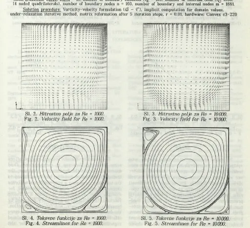
5. TESTNI PRIMER 5.1 Tok v odprti kotanji
5. NUMERICAL EXAMPLE 5.1 Driven Cavity Flow Test v odprti kotanji je standarden test za
preverjanje robno območne integralske sheme kakor tudi drugih sorodnih shem. Kvadratna kotanja vsebuje izotermni viskozni nestisljivi fluid. Namen analize je določitev gibanja fluida zaradi inducira nega gibanja na odprtem zgornjem robu. Analiza je bila izvedena za Re = 1000 in Re = 10000. Rezul tati postopka robnih elementov so primerjani z rešitvijo »benchmark«, ki jo je podal Ghia z me todo končnih elementov in uporabo zelo goste mre že (128 X 128 vozlišč). Primerjava pokaže zelo dobra ujemanja rezultatov obeh preračunov. Slika 1 prikazuje geometrijsko obliko problema, diskretizi- rano območje in robne pogoje. Sliki 2 in 3 prikazu jeta polje, sliki 4 in 5 pa grafe tokovne funkcije.
Sl. 1. Mreža, geometrija in robni pogoji.
Diskretni model: neenakomerna mreža. 41 x 41 vozlišč, linearna interpolacija za funkcijo, konstantna interpolacija
za odvod funkcije, razmerje mreže: Lm a x / L m jn = 10, število robnih elementov NE = 160, število notranjih celic
Nc = 1600. (4 vozliščni četverokotniki), število robnih vozlišč n = 160, število robnih in notranjih vozlišč m = 1681. Postopek reševanja: vrtinčno-hitrostna formulacija (čo - v*), impliciten izračun vrednosti v območju, pod-relaksacijska iterativna metoda, reformacija matrike po 5 iteracijah, r = 0,01, računalnik: Convex c3-220
Fig. 1 Mesh, geometry and boundary conditions
Pierete model: Non-uniform mesh, 41 x 41 nodes, linear interpolation for function, constant interpolation for flux.
Mesh gradation: L m a x / L m i n = 10, number of boundary elements NE = 160, number of internal cells Nc 1600,
(4 noded quadrilaterals), number of boundary nodes n = 160, number of boundary and internal nodes m = 1681. Solution procedure: Vorticity-velocity formulation (to - v“), implicit computation for domain values, under-relaxation iterative method, m atrix reformation after 5 iteration steps, r = 0.01, hardware: Convex c3-220
Fig. 2. Velocity field for Re = WOO.
SI. 4. Tokovne funkcije za Re = WOO. Fig. 4. Streamlines for Re = WOO.
SI. 3. Hitrostno polje za Re = 10000. Fig. 3. Velocity field for Re = 10000.
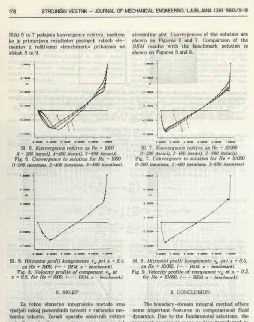
Sliki 6 in 7 podajata konvergenco rešitve, medtem ko je primerjava rezultatov postopek robnih ele mentov z rešitvami »benchmark« prikazana na slikah 8 in 9.
00 0 0 0 0 0 . 2 0 0 0 0 0 . 4 0 0 0 0 0 . 6 0 0 0 0 0 . 8 0 0 0 0 1 . 0 0 0 0 0
Sl. 6. Konvergenca rešitve za Re = 1000
(1 - 200 iteraci j. 4-400 iteraci j. 3 -8 0 0 iteraci j).
Fig. 6. Convergence to solution for Re = 1000
(1-200 iterations. 2 -400 iterations. 3 -8 0 0 iterations).
SI. 8. Hitrostni profil komponente vx pri x = 0,5, za Re = 1000, (----BEM. o - benchmark). Fig. 8. Velocity profile of component vx at X — 0 , 5 , for Re = 1 0 0 0 , (---BEM. o - b e n c h m a r k ) .
6. SKLEP
Za robno območno integralsko metodo smo vpeljali nekaj pomembnih novosti v računsko me haniko tekočin. Zaradi uporabe osnovnih rešitev več ali manj celotnega pojava prenesemo na rob obravnavanega območja, kar se kaže v stabilnosti in natančnosti numerične sheme. V primeru upo rabe Laplaceove ali difuzijske Greenove funkcije prenesemo celotno difuzijo na rob območja, med tem ko zajamemo konvekcijo z območnimi inte grali. Mnogo bolj učinkovita je numerična shema, ki je zasnovana na difuzijsko konvektivni Greenovi funkciji. Stabilnost numerične rešitve te sheme
streamline plot. Convergences of the solution are shown on Figures 6 and 7. Comparison of the BEM results with the benchmark solution is shown on Figures 8 and 9.
0 . 0 0 0 0 0 0 2 0 0 0 0 0 . 4 0 0 0 0 0 . 6 0 0 0 0 0 . 8 0 0 0 0 1 . 0 0 0 0 0
SI. 7. Konvergenca rešitve za Re = 10000
(1-200 iteracij. 2-400 iteracij. 3 -8 0 0 iteracij).
Fig. 7. Convergence to solution for Re = 10000
(1-200 iterations. 2 -400 iterations, 3-800 iterations).
SI. 9. Hitrostni profil komponente vx pri x = 0.5, za Re = 10000, (----BEM. o - benchmark).
Fig. 9. Velocity profile of component vx at x = 0.5, for Re = 10000, (----BEM. o - benchmark).
6. CONCLUSION