A low-power data acquisition system for geomagnetic observatories and variometer stations

https://doi.org/10.5194/gi-6-345-2017

© Author(s) 2017. This work is distributed under the Creative Commons Attribution 3.0 License.

A low-power data acquisition system for geomagnetic observatories

and variometer stations

Achim Morschhauser, Jürgen Haseloff, Oliver Bronkalla, Carsten Müller-Brettschneider, and Jürgen Matzka GFZ German Research Centre for Geosciences, Section 2.3: Geomagnetism, Telegrafenberg, 14473 Potsdam, Germany Correspondence to:Achim Morschhauser ([email protected])

Received: 3 March 2017 – Discussion started: 30 March 2017

Revised: 18 June 2017 – Accepted: 27 June 2017 – Published: 20 September 2017

Abstract.A modern geomagnetic observatory must provide data of high stability, continuity, and resolution. The INTER-MAGNET network has therefore specified quantitative crite-ria to ensure a high quality standard of geomagnetic observa-tories. Here, we present a new data acquisition system which was designed to meet these criteria, in particular with respect to 1 Hz data. This system is based on a Raspberry Pi em-bedded PC and runs a C++ data acquisition software. As a result, the data acquisition system is modular, cheap, and flexible, and it can be operated in remote areas with limited power supply. In addition, the system is capable of near-real-time data transmission, using a reverse SSH tunnel to work with any network available. The system hardware was suc-cessfully tested at the Niemegk observatory for a period of 1 year and subsequently installed at the Tatuoca observatory in Brazil.

1 Introduction

Geomagnetic observatories are known for providing contin-uous and high-quality geomagnetic field data (e.g. Matzka et al., 2010). These data are essential to understand the geo-magnetic field, its sources and its temporal variations (e.g. Chulliat et al., 2016). Amongst many other examples, ge-omagnetic observatories are an important source of reli-able long-term data to resolve secular variation over several decades to centuries (e.g. Wardinski and Holme, 2006; Jack-son et al., 2000), and they are essential to derive indices of geomagnetic activity (e.g. Menvielle et al., 2011) due to their fixed position on Earth. The main disadvantage, however, is their sparse spatial global coverage (Macmillan, 2007; Ras-son et al., 2010). The reaRas-son is the dependence on

infrastruc-ture such as a reliable power supply, facilities for continuous data transmission, as well as their dependence on human re-sources for maintenance tasks and manual absolute measure-ments. In particular, the availability of power and continu-ous data transmission remains a challenge in remote areas whereas the lack of absolute measurements might be accept-able for some applications such as magnetospheric studies or short-period magnetotellurics.

Since the digitization of geomagnetic observatories, effi-cient and reliable data acquisition systems had to be devel-oped. Such a system is responsible for digitizing the analogue output signal of the sensors, for timestamping the readings, and for filtering, storing, and transmitting the data. Due to the long life cycle of geomagnetic observatory installations, many of the currently used data acquisition systems have been developed in the 1980s and 1990s. In consequence, spare parts are more and more difficult to obtain, and mod-ern requirements with respect to power consumption, resolu-tion, and timestamping accuracy can hardly be fulfilled. For example, the MAGDALOG data acquisition system devel-oped at the GFZ German Research Centre for Geosciences (Linthe et al., 2009) runs on DOS, usually requires two ad-ditional PCs which increase power consumption, and limits the use of digital filters by its sampling rate of 2 Hz. For the above reasons, existing data acquisition systems are being modernized, including G-DAS used by BGS (Riddick et al., 2009), the system used by the Polish Academy of Sciences (Reda and Neska, 2016), and ENO3 used by IPGP (Chulliat et al., 2009), or newly developed such as the system MAR-COS/MARTHA of the Conrad observatory and the commer-cially available MAGREC-4 by MinGeo Ltd.

intend to fulfil the INTERMAGNET 1 Hz data standard (Tur-bitt et al., 2014). This system is designed to be highly mod-ular and flexible, allowing its adaptation to a particmod-ular lo-cation, existing infrastructure, and existing instrumentation. Also, easily available hardware such as the Raspberry Pi embedded PC (Upton and Halfacree, 2016) has been used whenever possible, and no custom-made electronic circuit boards are necessary. The system hardware was tested at the Niemegk geomagnetic observatory and installed at the Tatuoca geomagnetic observatory in Brazil (Morschhauser et al., 2017). These systems run a previous version of the data acquisition software which is mainly based on shell and Perl scripts along with C code for serial communication. The new software package is based on object-oriented C++and was tested in Niemegk, but more development and testing is nec-essary in order for it to be used in an operative environment. We believe that an efficient and versatile data acquisition sys-tem can only be developed with the support and experience of the community, and therefore encourage active participa-tion in the project by publishing the source code at a GFZ GitLab server under the Creative Commons licence for non-commercial use.

Details of the design criteria and functionality of the data acquisition system are presented in Sect. 2. Subsequently, the hardware is described in Sect. 3, and the data acquisition soft-ware is presented in Sect. 4. Finally, discussion and conclu-sions are given in Sect. 5.

2 Design criteria and functionality

A modern data acquisition system for geomagnetic observa-tories should meet a variety of requirements. Many of these requirements are included in the INTERMAGNET 1 Hz data standard (Turbitt et al., 2014); others result from operational conditions in remote areas.

INTERMAGNET specifies that the timestamping accu-racy for 1 Hz data should be better than 10 ms and that the deviation from a linear phase response should be less than 10 ms (Turbitt et al., 2014). This can be achieved by precise GPS or radio-controlled clocks in combination with good knowledge of the inherent time delays of the data acquisition system. In addition, the characteristics of the used analogue and digital filters should have a linear phase response and be well characterized. Also, INTERMAGNET requires a noise level of less than 10 pT Hz−1/2at 0.1 Hz. Amongst good sen-sors, this requires efficient anti-aliasing whilst the employed low-pass filter should not damp power in the passband. In-deed, INTERMAGNET requires at least 50 dB attenuation in the stop band of≥0.5 Hz (≤2 s), less than 3 dB attenuation in a transition passband of 8 mHz (120 s) to 0.2 Hz (5 s), and minimum attenuation in a passband of DC to 8 mHz (Turbitt et al., 2014). Therefore, specifically designed digital filters should be used along with high sampling rates, ideally faster than 120 Hz. Further, an analogue filter is recommended in

order to avoid aliasing of frequencies above the Nyquist fre-quency corresponding to half the sampling rate. In addition, INTERMAGNET demands a resolution of 1 pT along with a dynamic range of±3000 to 4000 nT depending on latitude (Turbitt et al., 2014). Still, the suggested dynamic range may be exceeded during extreme geomagnetic events (Thomson et al., 2011). In consequence, analogue-to-digital convert-ers (ADCs) with high resolution are necessary. For exam-ple, a DTU FGE with the largest available dynamic range of

±10 000 nT requires at least a 20 bit ADC in order to resolve 1 pT.

Other important design criteria which are not the sub-ject of the INTERMAGNET 1 Hz data standard, but which have been considered here, are described in the following. First, a fully operating geomagnetic observatory must guar-antee long-term stability of its data product. Therefore, cali-bration constants of the analogue output of the instruments must be stable and remain unchanged even after loss of power. In addition, the capability for real-time data trans-mission becomes more and more important, in particular for applications in geohazard monitoring and space weather, e.g. ground-induced currents (Viljanen et al., 2014; Bar-bosa et al., 2015). Finally, data gaps in operation should be avoided, requiring a system that is easy to operate, safely sur-vives power losses, close-by lightning strikes, and automati-cally restarts data acquisition as soon as power is available af-ter power loss. Continuous operation also requires that spare parts should be easily available and replaceable with com-monly available tools following simple procedures. In addi-tion, low power consumption of the whole system is essential for continuous operation, particularly in remote areas with an unreliable or no power grid.

In the following sections, we will present our approach to implement these design criteria with a modern C++ soft-ware package, a low-power and widely available embedded PC (Raspberry Pi), a modern ADC developed for geomag-netic observatories, and a flexible and modular system for backup and remote connectivity.

3 Hardware layout

The overall system layout can be divided into the power sup-ply chain and the data acquisition chain (Figs. 1 and 3) which we describe below. We required that the system should be easy to integrate in the existing observatory electronics which have previously been installed by GFZ in a number of obser-vatories worldwide (e.g. Korte et al., 2009). Still, we made sure that this requirement does not interfere with the flexibil-ity and easy integrabilflexibil-ity in other existing systems.

3.1 Data acquisition

embed-GPS RTC

Sensors and electronics

Variometer h ut

Electronics h ut

FMC

USB

RS232/485

Router FMC

Fibre optics

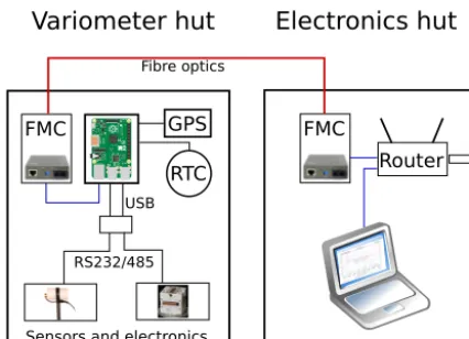
Figure 1.Schematic illustration of the data acquisition chain. On the left-hand side, the electronics in the variometer house is shown. These include the Raspberry Pi embedded computer as the cen-tral processing unit, the attached GPS sensor and real-time clock (RTC) for timekeeping, a fibre optics media converter (FMC), USB to RS232/485 converters, and the magnetometer sensors and elec-tronics. On the right-hand side, the electronics hut is shown where another FMC, an optional laptop or Raspberry Pi, and an optional router are located. See text for more details.

ded PC (Upton and Halfacree, 2016) which is responsible for timestamping, digital filtering, and buffering the data, as well as for communicating with the geomagnetic instruments and the corresponding ADCs. The Raspberry Pi was orig-inally developed as a tool to teach basic computer science in schools (Severance, 2013), but has found wide applica-tions also in science (e.g. Cox et al., 2013). Here, we use the Raspberry Pi model B+, which consumes maximally 3 W at 5 V (Upton and Halfacree, 2016) and which runs on an ARM processor clocked at 700 MHz along with 512 MB of shared memory. Further, the operating system and any data are stored on an internal SD card. Here, we have extended the Raspberry Pi by attaching an external real-time clock (RTC) (DS3231/AT24C32) to quickly restore the correct system time after power-loss, a GPS module (Microstack L80) in order to guarantee precise timekeeping in remote areas, and small serial to USB converters (FTDI USB-RS232-PCBA and FTDI USB-RS485-PCBA). Along with power supply and a fibre media converter (FMC), we enclose all peripher-als and the Raspberry Pi in an industrial plastic case for pro-tection (Fig. 2). This equipment is usually placed in the vari-ometer house in order to reduce cable lengths, and therefore must not influence the geomagnetic instruments. The data of most geomagnetic instrumentation is either available through a serial port (e.g. GEMSystem GSM magnetometers) or as an analogue signal (e.g. Technical University of Denmark (DTU) FGE variometer). In the former case, the Raspberry Pi will directly communicate with the instrument, and in the latter case, an ADC is required which we recommend to sup-port data sampling with at least 24 bit and 128 Hz. In our setup, we use a MinGeo ObsDAQ 24 bit ADC which

ad-ditionally allows for external triggering to improve timing accuracy, provides three independent input channels (non-multiplexed), can store pre-defined calibration constants, and is able to record housekeeping values such as voltage and temperature.

Ideally, any additional electronics should be kept in a sep-arate building which we will refer to as the electronics hut (Fig. 1). Data are transmitted from the Raspberry Pi to the electronics hut via rsync on a 15 min basis. For this pur-pose, a fibre optical cable is used instead of copper cables for two reasons: first, larger distances of up to 2 km (multi-mode) and 20 km (single (multi-mode) can be bridged compared to only a few hundred metres with twisted-pair copper ca-bles. Second, the optical transmission line serves as a gal-vanic isolation, avoiding, for example, induced currents due to close-by lightning strikes. For worldwide data transfer, we use a dedicated router to access the internet either via the mo-bile network or any local infrastructure, if available. In this way, a firewall can protect the observatory system, and a lo-cal UMTS USB modem can easily be integrated without hav-ing to worry about UMTS setthav-ings and modem drivers. Such a router is usually cheap, and consumes typically less than 5 W of power. Additionally, we use a laptop to locally back up the data and to graphically display the incoming data. In this way, the local observatory staff obtains immediate feed-back on the correct operation of the system. Even more, the observatory staff can manually store the absolute measure-ments on the laptop which are then transmitted automatically via rsync.

Apart from the described standard layout, some optional modifications may be useful. If power consumption is a se-vere issue, the laptop may be replaced by another Raspberry Pi with an optional TFT screen, or even be completely re-moved. In the latter case, however, no local backup of the data will be available. As well, the router may be removed and the data logger may directly be connected to the Inter-net. However, this solution is not recommended for security reasons and may only be applicable if the system is used as, for example, a temporary variometer station. Further, an ex-ternal HDD or SSD may be attached to the Raspberry Pi in order to increase storage capacity in case of extended loss of connectivity, or in order to provide a second local backup.

3.2 Power supply

RTC and GPS (below)

RPi

RS232/485

Power s upply GPS antenna

FMC (below RPi)

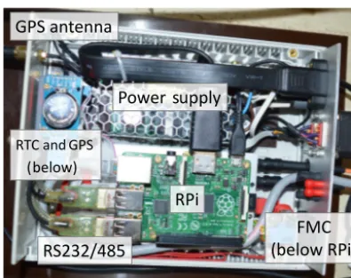
Figure 2.The Raspberry Pi in its housing as installed in Tatuoca (TTB). The most important components are labelled, i.e. the real-time clock (RTC), the power supply, the Raspberry Pi (RPi), the USB to RS232/485 converters, the fibre optics media converter (FMC), and the connector for the GPS antenna. The GPS module is located under the RTC and the FMC is located under the Rasp-berry Pi.

power grid, or various kinds of generators, may optionally be attached.

3.2.1 Power supply chain

A schematic overview of the power supply chain is shown in Fig. 3. The battery pack and generators will usually be situated in a separate housing far enough from the geomag-netic instrumentation in the variometer and absolute houses. For the effective transmission of electric energy, the 12 VDC output of the batteries will be transformed to higher-voltage AC power, usually 220–240 V. For example, if 15 W needs to be transmitted with a 1.5 mm2copper cable, power losses of 40 and 0.1 mW m−1are expected for 12 VDC and 220 VAC, respectively. As a positive side-effect, disturbing magnetic fields generated by DC currents will be avoided in this way. Also, alternating current allows us to use a well-tested and simple system of transformers developed in Niemegk in or-der to provide the required voltages for the operation of the proton and fluxgate magnetometers in the variometer house. Concerning the central data acquisition unit including the Raspberry Pi and the fibre optics media converter (FMC), the required 5 VDC power is provided by a commercial AC–DC power converter which is embedded in the data acquisition unit (Fig. 2). In addition, a suitable lightning protection (e.g. FURSE ESP 240-16A/BX) needs to be installed at both ends of the 220 VAC power line in order to protect the equipment from induced currents due to close lightning strikes.

The power consumption of a typical system with a DTU FGE as vector fluxgate magnetometer, a GEMSystem GSM-90F1 as scalar magnetometer, and a laptop is shown in Ta-ble 1, resulting in 40 W. Additionally, we add 10 % to ac-count for losses in the transformers and AC–DC

convert-Sensors and electronics

Variometer h ut Electronics h ut

3 x 1.5 mm2

PWI

12 VDC 220 VAC

Router Laptop LTP LTP

5 VDC

Figure 3.Schematic illustration of the power supply. On the right-hand side, the electronics hut is shown. The system is powered by solar cells and/or the power grid or generators. A power inverter (PWI) transforms 12 VDC of the buffer batteries to 220 VAC for transmission to the variometer hut. Also, the laptop and router are powered by 220 VAC. On the left-hand side, the variometer hut is shown where the Raspberry Pi, the sensors, and the electronics are powered via appropriate transformers and AC–DC converters. A lightning protection (LTP) is installed in both the variometer and electronics hut.

Table 1.Power consumption of a typical installation of the proposed data acquisition system.

Instrument I [mA]/U [V] Power [W] Comment

DTU FGE 1.5

GSM90F1 250/12 DC 3

Raspberry Pi 1000/5 DC 5

Router∗ 5

Laptop∗ 20

Power Inverter 5 φ >88 %

∗_{If power consumption needs to be reduced, the laptop and/or the router can be} removed. See text for details.

ers for the laptop and the Raspberry Pi data processing unit. Overall, this results in a maximum power consumption of less than 45 W. By replacing the netbook with a second Rasp-berry Pi and a small TFT screen, this number may be fur-ther decreased to 35 W. Optionally, the laptop may be com-pletely removed, resulting in a power consumption of less than 25 W.

3.2.2 Photovoltaic system

The required sizeBS of the batteries can be calculated

de-pending on the number of required daysND the system can

survive without sunshine and the overall power consumption P by

BS[Ah] =

P [W]ND[d]

0.3

24[h d−1]

if a maximum discharge depth of 30 % is assumed. At least, we require that ND=0.5 in order to survive the night. In

this case, BS≈3.3 Ah are necessary for each watt of

sys-tem power, i.e. 149 Ah for our syssys-tem. ForND=5, however,

these numbers increase to 33 Ah W−1and 1485 Ah, respec-tively. Concerning the solar panels, the necessary daily power productionPSDshould at least balance the daily power

con-sumption, i.e.PSD[Wh d−1]=P [W] 24 [h d−1]. In addition,

larger solar arrays are necessary in order to recharge empty batteries withinNRdays due toNDsuccessive days without

sunshine, i.e.

PSD[Wh d−1] =

_N

D[d]

NR[d] +1

P [W]24[h d−1]. (2)

ForND=2 andNR=2, this results inPSD≈3.8 kWh d−1

for the standard system withP =45 W. Now, the required nominal peak powerPWpof the solar cells can be calculated

from the minimum daily solar radiation G (e.g. Paulescu et al., 2012) at the given location, the inclination and az-imuth of the solar panels, and the ambient temperature (e.g. Almonacid et al., 2011).

4 Software layout

The data logger software is running on the Raspberry Pi un-der a Raspbian (Debian-un-derivate) Linux operating system. Still, it may be compiled with any C++11 ANSI compiler on different platforms as long as the underlying operating system is POSIX compatible.

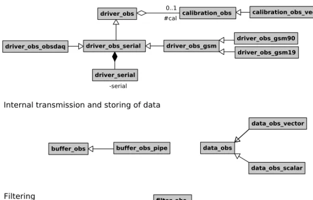
The software contains different abstraction layers, from more generic classes defining interfaces to more special-ized classes (Fig. 4). Further, the implemented classes can be grouped according to their functionality. First, we will describe the classes providing functionality to communicate with the geomagnetic instrumentation (drivers). Then, we will describe the timestamping of the incoming data, fol-lowed by a section on the filtering, storing, and internal trans-mission of the data. Finally, we will describe our current so-lution for data transmission to external servers.

4.1 Communication with instruments

The UML diagram for the classes needed to communicate with instrumentation at an observatory is shown in the upper part of Fig. 4. At the most abstract level, the software package provides an abstract class<driver_obs>which defines some compulsory interface methods such as taking a single mea-surement, taking continuous measurements in free-run mode, taking continuous measurements in triggered mode, and stopping continuous measurements. In free-run mode, the software will passively listen to incoming data. In triggered mode, the software will actively trigger the measurements at a specified frequency. Depending on the instrument, the ac-tive trigger may also be a PPS which is directly attached to

the instrument. Moreover, calibration constants of the instru-ment can be passed to the driver using the generic abstract class<calibration_obs>. An implementation for vector data is provided by the class<calibration_obs_vector>.

For communication using serial ports, we have imple-mented a generic serial driver class<driver_serial>which provides a convenient wrapper for serial communication functionality usingtermios. For example, a termination char-acter as used by many instruments can be set for receiving data on the serial port. Also, the system time of the first char-acter received can be passed for timestamping purposes.

Based on these classes, a generic class <driver_obs_serial>for communication with observatory instruments using the serial port has been developed. For example, this class provides functionality to automatically set the correct baud rate. Up to now, drivers for the MinGeo ObsDAQ ADC (<driver_obs_obsdaq>) and the GEMSys-tem GSM-90 and GSM-19 families (<driver_obs_gsm90> and <driver_obs_gsm19>) have been implemented. For these drivers, arbitrary sampling rates can be requested by the user, and the driver will automatically test if it is supported by the instrument. Further, additional drivers can be added in the future.

4.2 Timestamping and timekeeping

There are two different modes of timestamping that can be used depending on the capabilities of the attached instru-ment: the free-run mode, which works with any instrument, and the triggered mode. In free-run mode, the timestamp of incoming data is set according to the system time when the first byte is received. In this case, the timestamp criti-cally depends on the accuracy of the system time. Also, the timestamp includes a delay due to the transmission time of the data from the instrument to the data logger, and due to the processing time of the operating system on the data log-ger. We estimate that a timing accuracy of up to 1 ms can be achieved in free-run mode. For higher timing accuracy up to 0.1 ms, the triggered mode requires an ADC or geomagnetic instrument that can directly be synchronized to some pre-cise pulse, e.g. an attached GPS. Still, the exact timing accu-racy significantly depends on the chosen setup and should be tested with an instrument such as described in Rasson (2008). In addition, the overall time delay depends not only on the digital signal processing chain but also on the response func-tion and phase delay of the chosen geomagnetic instrument.

-serial

0..1 #cal

Internal transmission and storing of data

driver_obs_gsm

driver_obs_gsm19 driver_obs_gsm90

driver_obs_obsdaq driver_obs_serial

driver_obs

driver_serial

calibration_obs calibration_obs_vector

Drivers and timestamping

data_obs buffer_obs

data_obs_scalar buffer_obs_pipe

data_obs_vector

Filtering _{filter_obs}

Figure 4. UML diagram showing the relationships between classes of the C++data acquisition software. Please refer to the text for explanations and details.

that these are supported by the Linux GPS daemon gpsd. Sec-ondary time sources may include any close-by time servers.

4.3 Data logging and filtering

The instrument drivers described above store the data in a generic data class<data_obs>(middle part of Fig. 4). This generic class can hold timestamps only, and is extended by the classes<data_obs_scalar>and<data_obs_vector>to work with scalar and vector data, respectively. In addition to storing data, all data classes also provide methods for cal-culating the weighted mean and the median for a given data set.

For further processing, the data can be stored in a buffer that collects incoming data. For this purpose, a generic class <buffer_obs>is available, providing methods to push and pop objects of type<data_obs>. Such a buffer may be im-plemented in various ways. An easy and convenient solution is to use an ASCII representation of the data and to write to STDOUT. Now, STDOUT can be connected to STDIN of a processing program via the pipe command. This approach is implemented in the class<buffer_obs_pipe>. Also, STD-OUT may be split using theteecommand to store raw data at high sampling frequency in separate files. A more sophisti-cated approach to implement<buffer_obs>could consist of using a queue along with threaded processes to take the mea-surements and to process the data, or even to use a messaging protocol server, such as MQTT.

Up to now, a generic finite impulse response (FIR) digital filter and a median filter have been implemented in a class <filter_obs>for further processing the data (lower panel of Fig. 4). Also, we have implemented the filter suggested by

the PLASMON project which fulfils the INTERMAGNET specifications. This filter is a two-stage FIR filter that down-samples the data from 128 or 640 Hz to 1 Hz (Merényi et al., 2013). For input and output, the class<filter_obs> continu-ously reads the data from an input buffer and writes the fil-tered data to an output buffer, both of type<buffer_obs> Now, the data can be written to an ASCII file if an output buffer of type<buffer_obs_pipe>is used. If the data should be written to a binary file, or even transmitted in real time (e.g. using MQTT), a suitable class of type<buffer_obs> could be implemented.

4.4 Integration in operating system

The software package has to be integrated in the running op-erating system. For this purpose, a number of bash scripts and cronjobs are responsible. For example, these make sure to automatically start data acquisition at reboot and after power loss, backing up and compressing transmitted data, and to log any events such as starting and stopping the data logging software, NTP time information, or disk space availability. These tasks may also be accomplished by a service manager such assystemd. However, such service managers are usually more complex to administrate. Also, service managers differ for some distributions and have been replaced in the past, whereas cron and bash are available on all distributions.

4.5 Data transmission

A simple and reliable approach for secure data transmission is a file-based method where data is transmitted to a central server viarsyncandscp. In addition, a reverse SSH tunnel may be necessary if the data logger is protected by a firewall or assigned a dynamic IP address. On the side of the central server, a scheduler such ascroncan then be used to contact the data logger and to transmit the data on a regular basis.

Alternatively, and if real-time data access is required, a messaging protocol such as MQTT can be used (Bracke et al., 2017). Also, the data may be temporarily transferred to a central database in order to quickly extract, access, and process the latest data.

5 Conclusions and outlook

We have presented a data logging system for use at geomag-netic observatories and described its hardware design and software package. It is based on a Raspberry Pi embedded PC as the central data acquisition unit, without the need for any custom-made circuit boards. The software package is written in object-oriented C++ and runs on any POSIX-compliant operating system. Advantages of the system include its ver-satility and flexibility, its relatively low power consumption, and its compatibility with the INTERMAGNET 1 Hz stan-dard. We encourage the community to participate in its use and further development by making the C++ source code freely available under the creative commons license (see note on code availability below).

The hardware setup was successfully tested at the Niemegk geomagnetic observatory for about 1 year. Dur-ing this time, the Raspberry Pi was runnDur-ing almost contin-uously and we observed no problems concerning its relia-bility and starelia-bility in continuous operation. In addition, the system was installed at the Tatuoca observatory in Brazil (Morschhauser et al., 2017), where it was continuously run-ning from November 2015 until a lightrun-ning strike in Decem-ber 2016, and has been operational again since 20 Febru-ary 2017. To date, the Raspberry Pi data logger provides a reliable platform. However, the described C++ software package is under current development, and still requires thor-ough testing before it can be routinely installed at geomag-netic observatories. For example, more elaborate configura-tion files for calibraconfigura-tion constants and the triggered mode op-tion for the MinGEO ObsDAQ analogue-to-digital converter need to be implemented. Further, anticipated hardware im-provements include a battery-powered shutdown procedure, and the inherent time delay of the system still needs to be fully characterized.

We intend to install the proposed system in many of the ge-omagnetic observatories operated by GFZ or in cooperation with other institutes. Moreover, the modular design provides the potential to adapt the system to a variety of settings, e.g.

for electric field measurements, for repeat station surveys, for temporal variometer stations, or even for magnetometer cali-bration systems. Therefore, we would like to welcome contri-butions from other institutes and observatories, and strongly support a community-based effort towards a modern, afford-able, flexible, and reliable data acquisition system that can be freely used in many observatories.

Code availability. The C++software is freely available for non-commercial use under the Creative Commons licence at https: //gitext.gfz-potsdam.de/mors/GeomagLogger.git. Contributions are welcome, and the author should be contacted for access to the de-veloper branch.

Author contributions. AM wrote the paper and implemented the C++data acquisition software described here, OB developed a pre-vious versions of the data acquisition and transmission software, JH and CMB designed the hardware layout, JH installed the test sys-tem, and JM coordinated the activities.

Competing interests. The authors declare that they have no conflict of interest.

Special issue statement. This article is part of the special issue “The Earth’s magnetic field: measurements, data, and applications from ground observations (ANGEO/GI inter-journal SI)”. It is a re-sult of the XVIIth IAGA Workshop on Geomagnetic Observatory Instruments, Data Acquisition and Processing, Dourbes, Belgium, 4–10 September 2016.

Acknowledgements. We thank Stephan Bracke and Peter Crosth-waite for their detailed reviews and suggestions that helped to improve the manuscript. Also, we thank Jean Rasson and the team at the Dourbes Observatory for organizing the INTERMAGNET workshop in 2016.

The article processing charges for this open-access publication were covered by a Research

Centre of the Helmholtz Association.

Edited by: Jean Rasson

Reviewed by: Peter Crosthwaite and Stephan Bracke

References

Almonacid, F., Rus, C., Pérez-Higueras, P., and Hontoria, L.: Cal-culation of the energy provided by a PV generator. Comparative study: Conventional methods vs. artificial neural networks, En-ergy, 36, 375–384, https://doi.org/10.1016/j.energy.2010.10.028, 2011.

at a low-latitude region over the solar cycles 23 and 24: compari-son between measurements and calculations, J. Space Weather Space Clim., 5, A35, https://doi.org/10.1051/swsc/2015036, 2015.

Bracke, S., Gonsette, A., Rasson, J., Poncelet, A., and Hendrickx, O.: Automated observatory in Antarctica: real-time data transfer on constrained networks in practice, Geosci. Instrum. Method. Data Syst. Discuss., https://doi.org/10.5194/gi-2017-17, in re-view, 2017.

Chulliat, A., Savary, J., Telali, K., and Lalanne, X.: Acquisition of 1-second data in IPGP magnetic observatories, in: Proceed-ings of the XIIIth IAGA Workshop on Geomagnetic Observa-tory Instruments, Data Acquisition, and Processing, edited by Love, J. J., Vol. 1226, US Geological Survey, available at: https: //pubs.usgs.gov/of/2009/1226/ (last access: 1 May 2017), 2009. Chulliat, A., Matzka, J., Masson, A., and Milan, S. E.: Key

Ground-Based and Space-Ground-Based Assets to Disentangle Magnetic Field Sources in the Earths Environment, Space Sci. Rev., 206, 123– 156, https://doi.org/10.1007/s11214-016-0291-y, 2016. Cox, S. J., Cox, J. T., Boardman, R. P., Johnston, S. J.,

Scott, M., and O’Brien, N. S.: Iridis-pi: a low-cost, com-pact demonstration cluster, Cluster Comput., 17, 349–358, https://doi.org/10.1007/s10586-013-0282-7, 2013.

Jackson, A., Jonkers, A. R. T., and Walker, M. R.: Four centuries of geomagnetic secular variation from historical records, Philos. T. R. Soc. A, 358, 957–990, https://doi.org/10.1098/rsta.2000.0569, 2000.

Korte, M., Mandea, M., Linthe, H.-J., Hemshorn, A., Kotze, P., and Ricaldi, E.: New geomagnetic field observations in the South At-lantic Anomaly region, Ann. Geophys., 52, 65–81, 2009. Linthe, H.-J., Mandea, M., and Korte, M.: Installing a

Geomag-netic Observatory on St. Helena Island – a Special Challenge, in: Proceedings of the XIIIth IAGA Workshop on Geomagnetic Ob-servatory Instruments, Data Acquisition, and Processing, edited by Love, J. J., Vol. 1226, US Geological Survey, available at: https://pubs.usgs.gov/of/2009/1226/ (last access: 1 May 2017), 2009.

Macmillan, S.: Observatories, Overview, in: Encyclopedia of Ge-omagnetism and PaleGe-omagnetism, edited by: Gubbins, D. and Herrero-Bervera, E., 708–711, https://doi.org/10.1007/978-1-4020-4423-6_224, Springer Nature, 2007.

Matzka, J., Chulliat, A., Mandea, M., Finlay, C. C., and Qamili, E.: Geomagnetic Observations for Main Field Stud-ies: From Ground to Space, Space Sci. Rev., 155, 29–64, https://doi.org/10.1007/s11214-010-9693-4, 2010.

Menvielle, M., Iyemori, T., Marchaudon, A., and Nosé, M.: Ge-omagnetic Indices, in: GeGe-omagnetic Observations and Models, edited by: Mandea, M. and Korte, M., Vol. 5, IAGA Special So-pron Book Series, chap. 8, 183–228, https://doi.org/10.1007/978-90-481-9858-0_8, Springer, 2011.

Merényi, L., Heilig, B., and Szabados, L.: Geomagnetic Data Ac-quisition System Developed for the PLASMON Project, in: Pro-ceedings of the XVth IAGA Workshop on Geomagnetic Ob-servatory Instruments, Data Acquisition, and Processing, edited by: Hejda, P., Chulliat, A., and Catalán, M., 03/13, Boletín Roa, 2013.

Morschhauser, A., Soares, G. B., Haseloff, J., Bronkalla, O., Pro-tasio, J., Pinheiro, K., and Matzka, J.: The Magnetic Obser-vatory on Tatuoca, Belém, Brazil: History and Recent De-velopments, Geosci. Instrum. Method. Data Syst. Discuss., https://doi.org/10.5194/gi-2017-19, in review, 2017.

Paulescu, M., Paulescu, E., Gravila, P., and Badescu, V.: Solar Ra-diation Measurements, in: Weather Modeling and Forecasting of PV Systems Operation, 17–42, https://doi.org/10.1007/978-1-4471-4649-0_2, Springer Nature, 2012.

Rasson, J.: Testing the timing accuracy of 1s INTERMAGNET var-iometer, Tech. Rep. TN0004, INTERMAGNET, 2008.

Rasson, J. L., Toh, H., and Yang, D.: The Global Geomagnetic Ob-servatory Network, in: Geomagnetic Observations and Models, edited by: Mandea, M. and Korte, M., Vol. 5, IAGA Special So-pron Book Series, chap. 1, 1–25, https://doi.org/10.1007/978-90-481-9858-0_1, Springer Nature, 2010.

Reda, J. and Neska, M.: The One Second data collection system in Polish geomagnetic observatories, J. Ind. Geophys. Union, 2, 62–66, 2016.

Riddick, J. C., Rasson, J. L., Turbitt, C. W., and Flower, S. M.: INDIGO Digital Observatory Project, 2004–2008, in: Proceed-ings of the XIIIth IAGA Workshop on Geomagnetic Observa-tory Instruments, Data Acquisition, and Processing, edited by: Love, J. J., Vol. 1226, US Geological Survey, available at: https: //pubs.usgs.gov/of/2009/1226/ (last access: 1 May 2017), 2009. Severance, C.: Eben Upton: Raspberry Pi, Computer, 46, 14–16,

https://doi.org/10.1109/mc.2013.349, 2013.

Thomson, A. W. P., Dawson, E. B., and Reay, S. J.: Quantify-ing extreme behavior in geomagnetic activity, Space Weather, 9, S10001, https://doi.org/10.1029/2011sw000696, 2011.

Turbitt, C., St-Louis, B., Rasson, J., Matzka, J., Stewart, D., Lalanne, X., Schwarz, G., and Shanahan, T.: INTER-MAGNET Definitive One-second Data Standard, Technical Note 6, INTERMAGNET, available at: http://www.intermagnet. org/publications/im_tn_06_v1_0.pdf (last access: 1 May 2017), 2014.

Upton, E. and Halfacree, G.: Raspberry Pi User Guide, John Wiley & Sons Inc, 2016.

Viljanen, A., Pirjola, R., Prácser, E., Katkalov, J., and Wik, M.: Geo-magnetically induced currents in Europe, J. Space Weather Space Clim., 4, A09, https://doi.org/10.1051/swsc/2014006, 2014. Wardinski, I. and Holme, R.: A time-dependent model of