Fuzzy variants of prototype based clustering and classification algorithms
Geweniger, Tina
IMPORTANT NOTE: You are advised to consult the publisher's version (publisher's PDF) if you wish to cite from it. Please check the document version below.
Document Version
Publisher's PDF, also known as Version of record
Publication date: 2012
Link to publication in University of Groningen/UMCG research database
Citation for published version (APA):
Geweniger, T. (2012). Fuzzy variants of prototype based clustering and classification algorithms. Groningen: s.n.
Copyright
Other than for strictly personal use, it is not permitted to download or to forward/distribute the text or part of it without the consent of the author(s) and/or copyright holder(s), unless the work is under an open content license (like Creative Commons).
Take-down policy
If you believe that this document breaches copyright please contact us providing details, and we will remove access to the work immediately and investigate your claim.
Downloaded from the University of Groningen/UMCG research database (Pure): http://www.rug.nl/research/portal. For technical reasons the number of authors shown on this cover page is limited to 10 maximum.
Clustering and Classification Algorithms
Fuzzy Variants of Prototype Based
Clustering and Classification Algorithms
Proefschrift
ter verkrijging van het doctoraat in de
Wiskunde en Natuurwetenschappen
aan de Rijksuniversiteit Groningen
op gezag van de
Rector Magnificus, dr. E. Sterken,
in het openbaar te verdedigen op
maandag 22 oktober 2012
om 14:30 uur
door
Tina Geweniger
geboren op 13 maart 1976
te Altenburg, Duitsland
Prof. dr. T. Villmann Beoordelingscommissie: Prof. dr. T. Martinetz
Prof. dr. M. Opper Prof. dr. F. Rossi
Now, that all the work is done, there is a number of friends and collegues I wish to thank for their support, friendship, understanding, patience and their mere being there whenever needed. Thanks to (in reverse alphabetical order):
— Dietlind Zühlke — diss-sis: we got through it together — Prof. Thomas "Villy" Villmann —
thesis advisor: taught me to write scientifically and is a source of new ideas — Frank-Michael Schleif —
last minute proofreader: useful hints for final version — MESO Company —
employer: time off for writing my thesis — Wouter Lueks —
translator: without him there would not be a Dutch summary — Marika Kästner —
little diss-sis: proofreading, useful hints, and discussions — Klaus Geweniger —
husband: he believed in me — Prof. Michael Biehl —
"external" thesis advisor: fighting the dutch bureaucracy and excellent cooking — all members of the Mittweida–Bielefeld–Groningen research group —
Abbreviations and Symbols ix
1 Introduction 1
1.1 Scope . . . 2
1.2 Outline . . . 4
2 General notes about clustering and classification 5 2.1 Vector Quantization and Clustering . . . 5
2.1.1 Vector Quantization . . . 6 2.1.2 c-Means . . . 8 2.1.3 Self-Organizing Maps . . . 11 2.1.4 Neural Gas . . . 13 2.1.5 Fuzzy c-Means . . . 15 2.1.6 Median c-Means . . . 16 2.1.7 Affinity Propagation . . . 17
2.2 Prototype Based Classification . . . 19
2.2.1 Learning Vector Quantization – LVQ1 . . . 21
2.2.2 Learning Vector Quantization – LVQ2.1 . . . 23
2.2.3 Generalized LVQ . . . 23
2.2.4 Robust Soft LVQ . . . 26
2.2.5 Soft Nearest Prototype Classification . . . 27
2.2.6 Fuzzy Soft Nearest Prototype Classification . . . 29
2.3 Distance measures . . . 30
2.3.1 Euclidean metric and variants . . . 31
2.3.2 Divergences . . . 32
2.3.3 Kernel distances . . . 35 vii
2.3.4 Normalized Information Distance . . . 36
2.4 Validation measures for fuzzy clustering and classification . . . 36
2.4.1 Measures based on separation and compactness . . . 37
2.4.2 Rand index and related measures . . . 38
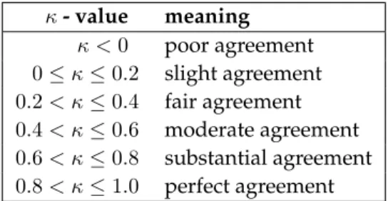
2.4.3 Cohen’ Kappa and Fleiss’ Kappa . . . 40
3 Fuzzy clustering for non-standard metrics 45 3.1 Relevance clustering with Fuzzy c-Means . . . 48
3.1.1 Incorporating a relevance parameter into FCM . . . 49
3.1.2 Divergences as dissimilarity measures . . . 50
3.1.3 Proof of concept . . . 54
3.1.4 Real world example – remote sensing data . . . 56
3.1.5 Conclusion . . . 62
3.2 Fuzzy median clustering . . . 62
3.2.1 Median Fuzzy c-Means . . . 63
3.2.2 Fuzzy interpretation of Affinity Propagation . . . 64
3.2.3 Artificial example – overlapping Gaussian distributions . . . 66
3.2.4 Real world example – psychological therapy transcripts . . . 69
3.2.5 Conclusion . . . 71
4 Fuzzy classification 73 4.1 Supervised learning . . . 76
4.1.1 Classifying fuzzy labeled data with FSNPC . . . 76
4.1.2 Fuzzy Robust Soft LVQ . . . 78
4.1.3 Artificial example – overlapping Gaussian distributions . . . 82
4.1.4 Real world example – barlay grain tissue sections . . . 85
4.1.5 Conclusion . . . 88
4.2 Semi–supervised learning . . . 89
4.2.1 Fuzzy Labeled NG . . . 90
4.2.2 Fuzzy Labeled SOM . . . 98
4.A Derivation of the F-FSNPC window rule . . . 102
4.B Derivation of the general FRSLVQ update rule . . . 104
5 Summary 109
Publications 115
Bibliography 119
Nederlandse samenvatting 131
v ∈ Rd d-dimensional input vector (resp. data sample)
w ∈ Rd d-dimensional prototype (resp. codebook vector, reference vector, exemplar)
d(v,w) general distance measure or dissimilarity
Exyz(...) cost function for algorithmXY Z
NC Number of classes or clusters
NP Number of prototypes (resp. codebook vectors, reference vectors,
exemplars)
NV Number of input vectors (resp. data samples)
P(V) data distribution in the input space
uj(vi) Membership assignment ofvito prototypewj
V Set of input vectors withV ={v1, . . . ,vNV} ⊂R
d
W Set of output vectors withW ={w1, . . . ,wNP} ⊂R
d
ANN Artificial Neural Network
CM c-Means
FAP Fuzzy Affinity Propagation
FCM Fuzzy c-Means
FLNG Fuzzy Labeled Neural Gas
FLSOM Fuzzy Labeled Self-Organizing Map
FRSLVQ Fuzzy Robust Soft Learning Vector Quantization FSNPC Fuzzy Soft Nearest Prototype Classifier
FSOM Fuzzy Self-Organizing Map
GLVQ Generalized Learning Vector Quantization
LVQ Learning Vector Quantization
M-CM Median c-Means
M-FCM Median Fuzzy c-Means
NG Neural Gas
NID Normalized Information Distance
NPC Nearest Prototype Classifier
R-FCM Relevance Fuzzy c-Means
RSLVQ Robust Soft Learning Vector Quantization SNPC Soft Nearest Prototype Classifier
SOM Self-Organizing Map
SVM Support Vector Machine
VQ Vector Quantization
Introduction
Prototype based clustering and classification is one specific topic in the field of ma-chine learning and artificial neural networks (ANN). Mama-chine learning in general is a branch of artificial intelligence and covers the whole field of algorithms which acquire knowledge based on experience. Thereby, it can be distinguished between symbolic learning and learning from examples. Symbolic learning is based on ex-plicit rules in combination with data samples and is also known as inductive logic programming. Algorithms modulating neural networks rely on data samples and a special type-dependend structure, and store the obtained knowledge implicitly within their specific structure.
To the family of ANNs belong graph based methods like Bayesian networks and Markov Random Fields, Spectral Clustering, and prototype based algorithms. In the following chapters the focus is laid on prototype based methods, especially those, where the prototypes are located within the class centers. Non class typical classi-fiers like Support Vector Machines (SVM) are not within the scope of this thesis.
There are three different learning paradigms to distinguish: unsupervised learn-ing, supervised learning and reinforcement learning. Unsupervised learning, in par-ticular clustering, groups data into sets of similar objects and is applicable for ex-plorative data mining, statistical data analysis, pattern recognition, and information retrieval to name just a few. There exists a variety of prototype based algorithms like c-Means (CM) (Ball and Hall 1967, MacQueen 1967), Fuzzy c-Means (FCM) (Dunn 1973, Bezdek 1980, Hathaway and Bezdek 1986), Self-Organizing Maps (SOM) (Ko-honen1990), Neural Gas (NG) (Martinetz et al. 1993), and others. The difference to supervised learning or classification is, that the data samples used to train the artifi-cial neural network are not labeled. Therefore, these algorithms are suitable dealing with data, where no class information is given. The algorithms allow a first inspec-tion of the data and help to discover hidden structures. In the machine learning context these groups of similar objects are called clusters.
Supervised learningrefers to algorithms, where during the training process avail-able class information of the data samples is taken into account. This class infor-mation is usually obtained with the help of domain experts. Based on the learned structure, it is possible to classify unknown data samples. For prototype based
clas-sifiers new data samples are assigned to the class of the closest prototype respec-tively class center or class typical representant. Well known examples are Learning Vector Quantization (LVQ) (Kohonen 1986) and variants thereof (Sato and Yamada 1996, Seo and Obermayer 2003), and other Nearest Prototype Classifiers (NPC).
The third learning paradigmreinforcement learningis not covered within this the-sis. Rather than learning immediately through examples, it requires an external feedback or signal which measures the current state of the system. However, the reward is not given instantanuosly, but with a time delay with respect to a cer-tain action, such that a given signal responses to an action many timesteps before. Based on this signal, the actions are adapted to gain maximum long term reward. (Sutton 1984)
In practical applications, data, which in fact belongs to different groups, i. e. clusters or classes, might be overlapping and therefore cannot be separated clearly. For this kind of data particular supervised and unsupervised methods have been developed, e. g. Fuzzy c-Means (FCM) (Dunn 1973, Bezdek 1980, Hathaway and Bezdek 1986), Fuzzy SOM (FSOM) (Bezdek et al. 1992), and Fuzzy Soft Nearest Pro-totype Classification (FSNPC) (Villmann, Schleif and Hammer 2006). There, the data points, or for FSNPC the prototypes, are partially assigned to the clusters respec-tively classes reflecting the uncertainty in the data and allowing insecure decisions. These overlapping data sets are referred to asfuzzy dataand the respective learn-ing schemes arefuzzy methods. Here, the termfuzzyrefers to probabilistic or possi-bilistic assignments1of data points to clusters or classes and has to be distinguished
from fuzzy sets or fuzzy logic. In the context of machine learning it islearning with uncertaintiesand, accordingly, fuzzy clustering respectively fuzzy classification can be understood as probabilistic or possibilistic clustering or classification.
1.1
Scope
The main theme of this thesis is to extend known prototype based methods for clus-tering and classification to handle fuzzy data. Since clusclus-tering and classification are two different learning paradigms with a slightly different meaning concerning fuzziness, they are treated separately. While a cluster solution is called fuzzy if the data belonging to different clusters are overlapping, a fuzzy classification is either based on overlapping classes or on fuzzy labeled training data or both, where the fuzzy class assignments can also be interpreted as assignment probabilities. In the case of clustering, this interpretation is not valid. Assume two clusters and two
1Probabilisticimplies, that the positive assignments of a data point to the clusters or classes sums up
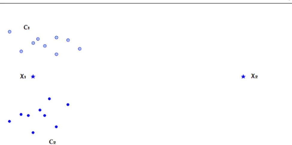
Figure 1.1:A situation in which the probabilistic assignment of membership is counterintu-itive for data sampleX2.
isolated data samples as depicted in Fig. 1.1. Intuitively, one would state that the probability of data sample 1 to belong to one of the clusters is higher than the proba-bility that data sample 2 belongs to them. The nature of clustering, being an ill-posed problem, suggests that each data sample has to be assigned to a cluster no matter how far away it is located. According to KRUSE ET AL. (Kruse et al. 2007) a better
formulation is:If a data sample has to be assigned to a cluster, then with the probabilityP
to clusterC.
A special challenge is to evaluate the obtained fuzzy clusterings and it is neces-sary to develop appropriate validation measures along with the algorithms. There-fore, a modification of the Fleiss’ Kappa Value, which is applicable for fuzzy solu-tions, is presented. Although intended for the verification of classificasolu-tions, it can also be applied to fuzzy cluster solutions.
Another aspect covered within this study is relevance learning versusrelevance clustering. Relevance learning can be incorporated into classification algorithms to improve the separation of the classes. It results in the identification of less relevant vector components, which can be necglected to reduce the number of input dimen-sions (Hammer and Villmann 2002).Relevance clusteringrefers to a weighting of the input dimensions to enhance the cluster solution in terms of separation and com-pactness.
Further, in articles concerning the above mentioned prototype based methods often a phrase like"the Euclidean distance is used but any other dissimilarity measure can be applied as well"can be found. In this thesis some examples of non-standard metrics have been explored. For example section 3.1 demonstrates the usefulness and applicability of generalized divergences to cluster functional data. To cluster
non-vectorial data like text documents a median variant of FCM is introduced in section 3.2. In the there presented example the Kolmogorov complexity (Bennett et al. 1998, Vitányi and Li 2000), see also section 2.3.4, is applied to obtain the dis-similarities beforehand. The algorithm itself works with the provided dissimilarity matrix.
1.2
Outline
In the following chapter"2 General notes about clustering and classification"some of the most important prototype based cluster algorithms and classification methods are introduced. Among them are the well-known c-Means (CM), Neural Gas (NG), and different variants of Learning Vector Quantization (LVQ). The purpose of this chapter is to establish a comprehensive foundation including algorithms, cost func-tions, and syntax and notation conventions concerning those approaches, which will be relevant in the following chapters. Further, alternative distance measures as well as measures for the validation of clustering and classification results are presented. Section 2.4.3 contains a proposal of an extension of the Fleiss’ Kappa Index, which allows the evaluation of fuzzy clusterings and classifications.
In chapter"3 Fuzzy clustering for non-standard metrics"fuzzy variants of the Means algorithm, e. g. Median Fuzzy Means (M-FCM) and Relevance Fuzzy c-Means (R-FCM), and a fuzzy interpretation of Affinity Propagation (AP) are pro-posed. The main property of M-FCM and FAP is, that both are based on mere simi-larities respectively dissimisimi-larities between the data samples. No further knowledge about special features of the data points themselves is required. Therefore, these cluster algorithms are applicable for non-metric data. The R-FCM algorithm in turn is designed to adapt the influence of specific data dimensions by manipulating the metric properties to improve the clustering in terms of separation and compactness. Further it is demonstrated that the usually used Euclidean metric can be substituted by some other dissimilarity measure like a divergence.
Chapter"4 Fuzzy Classification"first introduces fuzzy variants of the Robust Soft LVQ and Soft NCP. Thereby, the class labels are assumed to be probabilistic assign-ments to the classes. Beside the derivation of the update rules, for both algorithms representative examples are provided. Further two semi-supervised fuzzy learn-ing algorithms are proposed: Fuzzy Labeled SOM (FLSOM) and Fuzzy Labeled NG (FLNG). For these two also the theoretical aspects of the concept of relevance learn-ing are presented.
Finally, the last chapter provides a summary and conclusions, points out open questions, and brings up ideas for future work.
comparison of fuzzy classifiers,”in M. Verleysen (ed.), Proc. Of European Symposium on Artificial Neural Networks (ESANN 2009), d-side publications, Evere, Belgium, pp. 269-274, 2009.
Chapter 2
General notes about clustering
and classification
Abstract
This chapter provides a general introduction into the field of clustering and classification. The basic concepts of unsupervised and supervised learning algorithms relevant in the following chapters are presented along with annotations concerning used symbols, syn-tax, and notation conventions. Furthermore, a number of suitable distances respectively dissimilarities and validation measures are specified.
This chapter covers the established methods and measures essential for the follow-ing chapters. The first two sections 2.1 and 2.2 refer to prototype based cluster-ing and classification methods. Thereafter, different metric and non-metric distance measures are introduced in section 2.3, and finally, section 2.4 is concerned with a variety of validation measures applicable to fuzzy clustering and classification.
2.1
Vector Quantization and Clustering
Vector Quantization (VQ) in general is a prototype based learning scheme which can be applied for the sparse representation of unlabeled data. It is also referred to as unsupervised learning and used for the compression of very large data sets. Thereby, each cluster or group of similar objects is represented by one or more pro-totypes. These prototypes are located within the input space of the data samples. The main task of VQ algorithms is to describe the underlying data as close as possi-ble. Respective information about the relationship between data points or between data points and prototypes are taken into account, for example dissimilarities or neighboorhood rankings.
In the following, the first section provides the basic concepts of VQ, and after-wards some well known cluster algorithms are described in more detail. The last
two methods – Median c-Means and Affinity Propagation – work with non-vectorial data and, therefore, are no vector quantizers in this sense. Yet, since they are also intended to cluster large data sets they are included into this chapter.
2.1.1
Vector Quantization
As mentioned before, VQ is among others a method used for data compression. Possibly high-dimensional data vi ∈ Rd given by the datasetV = {v1, ...,vNV}
are mapped to a finite index setA = {1, . . . , NP}, which is associated with a set
W ofNP codebook vectors (prototypes)wj ∈ Rd. The codebook vectors are also
called reference vectors. The setW respectivelyAis substantially smaller thanV,
NP < NV, and each data samplevi is represented by the closest codebook vector
ws(vi). Formally this mapping can be stated as
ΨV→A:vi7−→s= argmin j∈A
(d(vi,wj)) (2.1)
whered(vi,wj)usually is the squared Euclidean norm1
d(vi,wj) = kvi−wjk2
= (v−w)2. (2.2)
The mapping ruleΨV→A(2.1) realizes awinner takes allrule, where each codebook
vectorwjrepresents a voronoi cell. All data samples within this receptive field
Rj={vi|ΨV→A(vi) =j} (2.3)
are mapped to the respective codebook vectorwj.
The crucial point in Vector Quantization is to find optimal codebook vectors to represent the data as accurate as possible. One way is to minimize the average expected square of the quantization error
EV Q= Z
d(v,ws(v))P(v)dv (2.4)
whereP(v)is the continuous propability density of the data distribution within the input spaceV. For discrete data the integral is reduced to a sum over all samples. A simple method to minimize (2.4) is to reposition the codebook vectors following a
1Throughout this work, the termd(v,w)is used as a general distance or dissimilarity measure.
Al-though most algorithms presented in this section are originally based on the squared Euclidean distance
d(v,w) = (v−w)2=
P
k(vk−wk)2, this is considered as a special case only and indicated seperately
where appropriate. If the general termdistanceis used, a (dis)similarity measure rather than a
stochastic gradient descent as described by KUSHNER&CLARK(Kushner and Clark 1978). This method was applied by LINDE, BUZOand GRAY, who developed the
LBG-algorithm 2.1.1a (Linde et al. 1980). Starting with (random) initial valueswj(0)
and updatingwjbased on prior values ofwjaccording to
wj(t+ 1) =wj(t) + ∆wj (2.5)
the algorithm converges for small learning rates0 < ε ≪ 1 to a local minimum (Linde et al. 1979). The parameter t indicates successive time steps and ∆wj is
obtained according to ∆wj = −ε 2· ∂EV Q(W) ∂wj = −ε 2· ∂ ∂wj Z d(v,ws(v))P(v)dv (2.6) which leads as a stochastic gradient to
∆wj = −ε·
∂d(vi,ws(vi))
∂wj (2.7)
for givenvi. If it is not indicated otherwise, the formula∂E∂wV Qj is an abbreviation for
this stochastic gradient.
Algorithm 2.1.1a – Standard Vector Quantization (VQ) „LBG–Algorithm”
1. Initialize the codebook vectorswj∈W randomly
2. Determine all updates∆wjaccording to eq. (2.7)
∆wj =−ε·
∂d(vi,ws(vi))
∂wj
3. Update all prototypeswjaccording to eq. (2.5)
wj(t+ 1) =wj(t) + ∆wj
4. Repeat steps 2. – 4. until convergence or manual stop
Since generally the data distribution P(vi)is not known, equation(2.5) can be
reformulated as
with
∆ws(vi)=−ε·
∂d(vi,ws(vi)(t))
∂ws(vi)(t)
(2.9) which is independent of P(vi) and leads to an approximation of the integration
(Linde et al. 1980). The complete algorithm is given in Alg. 2.1.1b. The respective update rule based on the Euclidean norm (2.2) yields
∆ws(vi)=ε·(vi−ws(vi)). (2.10)
Algorithm 2.1.1b – Standard Vector Quantization (VQ)
1. Initialize the codebook vectorswj∈W randomly
2. Present an input vectorvi
3. Determine thewinnerrespectively the best matching unitws(vi)according
to eq. (2.1)
s(vi) = argmin j′∈A
kvi−wj′ k
4. Update thewinnerws(vi)according to eq. (2.9)
ws(vi)(t+ 1) =ws(vi)(t)−ε·
∂d(vi,ws(vi)(t))
∂ws(vi)(t)
5. Repeat steps 2. – 5. until convergence or manual stop
After the presentation of all data points the codebook vectorswj are positioned
in the center of gravity of their respective receptive field. Problems in the stability of the behaviour of the algorithm are known to arise. These are caused by discontinous jumps of the indexs(vi), which might occur during the update of the codebook
vectors.
2.1.2
c-Means
The c-Means (CM) algorithm (also referred to as k-Means) is a simple and intuitive clustering method. It is a vector quantizer and as the name implies, this algorithm
groups a dataset intocdistinct clusters, where each cluster is represented by a pro-toype wj ∈ Rd located at the mean, i. e. the center of gravity, of the respective
cluster. There exists a batch as well as an online version.
Online c-Means For the case that the data distribution is not known a priori MAC
-QUEEN proposed an online version of the c-Means algorithm (MacQueen 1967),
where the data points are presented one after the other. At each time step a data pointviis assigned to the closest prototypewjbased on a distance functiond(vi,wj)
and only this prototypewj is repositioned to the mean of the cluster. The method
is straightforward and optimizes the general cost function given in equation (2.4) by stochastic gradient descent. The online update of all cluster centerswjis
deter-mined by
∆wj=ε·δj,s(vi)·
∂d(vi,wj)
∂wj (2.11)
whereε is the step size andδj,s(vi) the Kronecker delta, which equals1 iff wj is
the best matching prototype. For the special, originally proposed case, where the squared Euclidean distance is applied, this update rule can be formulated as
∆wj=−ε·δj,s(vi)·(vi−wj) (2.12)
Batch c-Means If the data distributionP(V)is known a priori, the batch version proposed by BALL & HALL (Ball and Hall 1967, Ball and Hall 1965) can be used. The (heuristic) objective function to be minimized yields
ECM = NV X i=1 NP X j=1 uj(vi)·d(vi,wj) (2.13)
The setU = {uj(vi)}, whereuj(vi)is used as an abbreviation for u(vi,wj),
de-fines the crisp membership of data pointvi ∈Rdto clusterwjand is bound to the
restrictions uj(vi)∈ {0,1} and NP X j=1 uj(vi) = 1. (2.14)
As before,d(vi,wj)denotes the distance between data pointviand prototypewj.
In the original proposal by BALL& HALL(Ball and Hall 1965) the squared Euclidean distance was used, but other non-negative dissimilarity measures might be suitable as well. A selection of different distance measures is presented in section 2.3.
Assignment updatewith fixed prototypeswj
uj(vi) =
1 if d(vi,wj) = min{d(vi,w1), . . . , d(vi,wNP)}
0 otherwise (2.15)
Prototype updatewith fixed assignmentsuj(vi)and based on the squared
Eu-clidean distance wj = PNV i=1uj(vi)·vi PNV i=1uj(vi) (2.16) Algorithm 2.1.2 – c-Means (CM)
1. Initialize the protoypeswj ∈W randomly
2. Calculate the membershipsuj(vi)of all datapointsvito all prototpyes
wjaccording to eq. (2.15)
uj(vi) =
1 if d(vi,wj) = min{d(vi,w1), . . . , d(vi,wNP)}
0 otherwise
3. Update the prototypeswjaccording to (2.16)
wj= PNV
i=1uj(vi)·vi PNV
i=1uj(vi)
4. Repeat steps 2. – 4. until convergence or manual stop
Although both version of the c-Means algorithm always converge, they might not find the optimal clustering, since they tend to get stuck in local minima (Duda and Hart 1973). Therefore it is necessary to perform several runs with different totype initializations. To select the initial prototypes several methods have been pro-posed. One of these suggests to take an appropriate number of data points as initial prototypes, or another method recommends to pick random points from the small-est (hyper-)box that encloses all data (Simpson 1993). A more sophisticated initial-ization method based on Latin hypercube sampling has been proposed by MCKAY
2.1.3
Self-Organizing Maps
Self Organizing Maps (SOM) are also known as Kohonen Maps since they where introduced by KOHONEN(Kohonen 1990). They belong to the most popular data
mining and visualization methods. Possibly high-dimensional data samples are nonlinearly mapped to a low-dimensional, typically two-dimensional grid. There, the topology of the original data is preserved. This grid or map constitutes a dis-crete representation of data samplesvi ∈Rd, i= 1, ...., NV. The nodes of the map
act as the prototypeswj ∈ Rdand their position within the usually rectangular or
hexagonal(actually triangular) grid is fixed. The training itself is administered by an unsupervised learning scheme based on vector quantization und uses a neighbor-hood function to preserve the topological properties of the input space.
The original model proposed by KOHONENwas improved by HESKES(Heskes 1999). According to (Heskes 1999) this modified method usually leads to almost the same results as the original SOM, yet additionally a cost function can be established, which makes this model feasible for continuous data distributions P(V). In the following only HESKES’ model is described.
A SOM consists of a setAofNPneuronsj, which are equipped with weight
vec-torswjrepresenting the prototypes. The neurons are arranged on a lattice structure,
which determines the neighborhood relationN(j, l)of neuronjandl. The mapping description of a trained SOM is defined by
Ψv→A:v7−→s(v) = argmin j∈A X l∈A hσ(j, l)d(v,wl) (2.17) where hσ(j, l) = exp −N(j, l) σ2 (2.18) describes the neighborhood cooperation with rangeσ > 0. The dissimilarity spec-ifyingd(vi,wj)is an appropriate differentiable distance measure, usually the
stan-dard Euclidean norm. In this method, an input is mapped onto that positionj =
s(vi)of the SOM, where the distanced(vi,wj)is at a minimum. Thereby the
av-erage over all neurons according to the neighborhood is taken into account. The neurons(vi)is referred to as thewinner.
A randomly initialized SOM is trained by sequential stochastic presentation of data pointsvi ∈V. At each time step the closest neurons(vi)according to (2.17) is
determined and the weights of neighboring neurons are adapted by ∆wj=−εhσ(j, s(vi))
∂d(vi,wj)
with a learning rateε > 0andε→0. This adaptation follows a stochastic gradient descent of the cost function introduced by HESKES(Heskes 1999):
ESOM = 1 C(σ) Z P(V) NP X j=1 δj,s(vi) NP X l=1 hσ(j, l)·d(vi,wl)dvi (2.20)
whereσis decreased with successive time steps, andδj,s(vi)is the Kronecker symbol
checking the identity ofjands(vi).
Algorithm 2.1.3 – Self-Organizing Map (SOM) HESKES
1. Initialize the neurons weightswjrandomly
2. Present a data pointviand identify thewinnerneuron (best matching unit)
s(vi)according to eq. (2.17) s(vi) = argmin j∈A X l∈A hσ(j, l)d(vi,wl)
3. Update the weights of the neurons in the neighborhood of thewinners(vi)
according to eq. (2.19), i. e. pull them closer to the input vector wj(t+ 1) =wj(t)−εhσ(j, s(vi))
∂d(vi,wj(t))
∂wj(t)
4. Repeat steps 2. – 4. until convergence or manual stop
One main aspect of SOMs is the visualization ability of the resulting map due to its topological structure (Villmann et al. 1997). Under certain conditions the re-sulting non-linear projectionΨv→Agenerates a continuous mapping from the data
spaceV onto the grid structureA. This mapping can mathematically be interpreted as an approximation of the principal curve or its higher-dimensional equivalents (Hastie and Stuetzle 1989). Thus, similar data points are projected on prototypes which are neighbored in the grid spaceA. Further, prototypes neighbored in the lattice space code similar data properties, i. e. their weight vectors are close together in the data space according to the applied metric. This property of SOMs is called topology preserving (or topographic) mapping realizing the mathematical concept of continuity (Villmann et al. 1997).
2.1.4
Neural Gas
The Neural Gas (NG) algorithm by MARTINETZ, BERKOVICH & SCHULTEN
(Mar-tinetz et al. 1993) is a highly efficient clustering algorithm. As for the algorithms in the previous sections the goal is to find prototypeswj∈Rd, j= 1, . . . , NP to
repre-sent continuous data pointsv∈Rdwhich are distributed according to an underly-ing distribution as accurate as possible. Thereby, as known for SOMs, the neighbor-hood of the prototypes is taken into account, yet without restricting the prototypes to fixed grid positions. Instead, a rank function based on the distances between the prototypeswiand data pointsvis introduced. Therefore, the dynamics of the
pro-totypes during the adaption process resemble the dynamics of Brownian particles moving in a potential determined by the data density (Martinetz et al. 1993). A ma-jor advantage of this algorithm compared to c-Means is, that the NG is insensitive to the prototype initialization.
The cost function to minimize is given by
EN G= 1 C(σ) NP X j=1 Z hσ(kj(v, W))·d(v,wj)P(V)dv. (2.21)
In the original proposal the Euclidean distance was used ford(v,w). The function
kj(v, W) =|{wk|d(v,wk)< d(v,wj)}| (2.22)
denotes the rank of the prototypes sorted according to their distances to the respec-tive data pointv. The neighborhood functionhσ(t)returns a maximum value for
kj(v, W) = 0and decreases to zero for higher ranks. Commonly, a Gaussian shaped
curvehσ(t) = exp(−t/σ)with neighborhood rangeσ >0is chosen. The
normaliza-tion constantC(σ) =PNP
j=1hσ(kj)depends only onσ.
The learning is accomplished by stochastic gradient descend with respect towj.
Given a data pointvthe update rule for prototypewjyields
∆wj=−ε·hσ(kj(v, W))· ∂d(v,
wj)
∂wj
(2.23) whereεis the learning rate withε >0. The neighborhood rangeσis decreased dur-ing the traindur-ing, which ensures independence of the initialization at the beginndur-ing of the training and optimizes the quantization error towards the end. Forσ → 0 the update rule is equivalent to the c-Means update rule eq. (2.11), and forσ 6= 0 all prototypes within the range ofσ are proportionally updated, i. e. not just the winner, but also the second, third, etc. ranked prototype (Martinetz et al. 1993).
Since its proposal the NG algorithm has been subject to extensive research and a number of variants have been developed. Prominent extensions are the Growing
Algorithm 2.1.4 – Neural Gas (NG)
1. Initialize the protoypeswj ∈W randomly
2. Present a randomly chosen data pointv 3. Update all prototypes according to eq. (2.23)
wj(t+ 1) =wj(t) +ε·hσ(kj(v, W))·
∂d(v,wj(t))
∂wj(t)
4. Repeat steps 2. – 4. until convergence or manual stop
Neural Gas (Fritzke 1995), the Supervised Neural Gas (Villmann and Hammer 2002, Hammer et al. 2005), the Kernel Neural Gas (Qin and Suganthan 2004a), and the Batch Neural Gas (Cottrell et al. 2006). Since the batch variant is of interest in section 4.2.1, a short review of the algorithm will be presented in the following.
According to COTTRELL ET AL. (Cottrell et al. 2006) the Neural Gas cost function
for discrete datavi∈Rd, i= 1, . . . , NV can be approximated by
EN G_Batch= 1 C(σ) NP X j=1 NV X i=1 hσ(kj(vi, W))·d(vi,wj). (2.24)
The quantitieskij := kj(vi, W)are now treated as hidden variables with the
con-straint, that the valueskij(j =i, ..., NP)constitute a permutation of{0, . . . , n−1}
for each data pointvi. Since the cost function depends on the hidden variableskij
and the prototypeswj, it has to be optimized with respect tokij andwj yielding
alternating adaptation steps:
Determine the ranks of the prototypeswj
kij =|{wl|d(vi,wl)< d(vi,wj)}| (2.25)
Update the prototypes based on fixed rankskijaccording to eq. (2.23)
Using the squared Euclidean distance this update can be formulated as wj = PNV i=1hσ(kij)·vi PNV i=1hσ(kij) (2.26) As known from other batch algorithms, before the update can take place all data samples have to be presented. Usually only a few, i. e. 10 to 100, adaptation steps are necessary.
2.1.5
Fuzzy c-Means
The Fuzzy c-Means (FCM) is an extension of the standard c-Means algorithm and was proposed by DUNN(Dunn 1973) and further on extensively discussed and im-proved by BEZDEK(Bezdek 1980), HATHAWAY(Hathaway and Bezdek 1986,
Hath-away et al. 1989) and others (Cannon et al. 1986, Ismail and Selims 1986). It is also an unsupervised learning scheme which aims to minimize an objective function by alternating update steps for prototypes and cluster memberships. The membership assigning data pointvito prototypewjnow is no longer crisp, i. e. a data point can
be assigned to one or more clusters. This assignment can either be possibilistic or probabilistic depending on the contraints put onuj(vi):
• probabilistic: uj(vi)≥0 with PjN=1P uj(vi) = 1, ∀i∈ {1, . . . , NV}
• possibilistic: uj(vi)∈[0,1]
Throughout this work only the probabilistic version will be persued. Therefore theNV ×NP matrixU with the elementsuj(vi)now is a probabilistic cluster
parti-tion ofV. The respective objective function to minimize is given by
EF CM = NV X i=1 NP X j=1 uj(vi)m·d(vi,wj) (2.27)
The exponentm ∈ (1,∞)regulates thefuzziness. For0 ←mthe assignments
con-verge to crisp decisions, wheras m → ∞ forces equally distributed assignments. Usually thefuzzinessis set to1.2≤m≤2. (Bezdek 1980)
Analogously to the standard c-Means the updates for the assignments uj(vi)
and the prototypeswj follow an alternating optimization scheme, yet also take the
fuzzinessminto account:
Assignment updatewith fixed prototypeswj
uj(vi) = 1 PNP k=1 d( vi,wj) d(vi,wk) 1 m−1 = m−p1 d(v i,wj)−1 PNP k=1 m−p1 d(v i,wk)−1 (2.28) Prototype updatewith fixed assignmentsuj(vi)
wj = PNV i=1uj(vi)m· ∂d(vi,wj) ∂wj PNV i=1uj(vi)m (2.29)
The update rules (2.28) and (2.29) are derived as solutions of the Lagrange mini-mization problem LF CM(λ) = EF CM+ NV X i=1 λi NP X j=1 uj(vi)−1 = 1 2 NP X j=1 NV X i=1 uj(vi)m·d(vi,wj) + NV X i=1 λi NP X j=1 uj(vi)−1 (2.30) For the special case of the quadratic Euclidean distance (2.2) eq. (2.29) yields
wj = PNV i=1uj(vi)m·vi PNV i=1uj(vi)m (2.31)
2.1.6
Median c-Means
The Median c-Means (M-CM) is another variant of the classical c-Means (Bezdek 1981). Yet, in contrast to the classical c-Means, the requirement that the data samples have to be embedded in a metric or vector space has been dropped. It is merely necessary to have some dissimilarity defined between the data samples, whereby this dissimilarity should follow the common sense understanding of dissimilarity (P˛ekalska and Duin 2005). The clustering now restricts the prototypes to be data samples itself: the algorithm determines a set W = {w1, . . . , wNP} where W ⊂
V. Instead of a distance functiond(vi, wj)now only a dissimilarity matrixD with
NV ×NV elements has to be provided. The elements are referred to asd(vi, vk)and
Dis assumed to be complete and symmetric.
LetPbe the index setP ={1, . . . , NP}for the prototypes andS={1, . . . , NV}
the index set for the data samples, then the mapping
I(i) :S→P (2.32)
specifies the winner index for a given data samplevi. This winner index refers to
the index of the prototype with minimum distance tovi:
I(i) = argmin
j∈P
d(vi, wj) (2.33)
Since the prototypeswjare restricted to be data samples, the similaritiesd(vi, wj)are
given by the distance matrixD. LetJ(j)denote the respective data index defining a bijective mapping
then the winner rule (2.33) can be written as
I(i) = argmin
j∈P
d(vi, wJ(j)) (2.35)
and thus the cost function for M-CM is given by
EM−CM = 1 2 NV X i=1 NP X j=1 ui,I(i)·d(vi, vJ(j)) (2.36) = 1 2 NV X i=1 d(vi, vJ(I(i))) (2.37)
where the characteristic functionui,I(i) = 1iff the data sampleviis represented by
prototypewI(i)which is equivalent with data samplevJ(I(i)).
Analogously to the in section 2.1.2 described c-Means algorithm, the optimiza-tion of the Median c-Means follows an alternating update of prototypes and assign-ments:
1. Assignment update: determine for each data samplevi∈V the winnerI(i)∈P
according to the minimum rule (2.33)
2. Prototype update: choose new prototypeswj =vlaccording to
l= argmin l′ NV X i=1 ui,l′·d(vi, vl′). (2.38)
Compared to the standard c-Means this median variant achives a considerable speed-up especially for large data set, since repeated calculations of distances be-tween data samples and prototypes can be skipped. Instead, the required dissimi-larities are obtained from the distance MatrixDwhich has to be provided.
The major drawback is the restriction to use data samples as prototypes. Es-pecially dealing with disjunct clusters leads to an only suboptimal solution. The prototypes have to be initialized carefully to avoid getting stuck in local minima.
2.1.7
Affinity Propagation
Affinity propagation as proposed by FREY& DUECK(Frey and Dueck 2007) is
an-other prototype based clustering algorithm, yet in contrast to the an-other algorithms it is based onsimilarities between data samples. It has been successfully applied for face recognition, the optimization of flight connections based on traveling time, to detect genes in microarray data, and to identify representative sentences in a manuscript (Frey and Dueck 2007).
The data points can be interpreted as nodes in a network and initially all of them are treated as prospective canditates for prototypes. By exchanging real-valued mes-sage simultaneously, the data pointscommunicatewith each other and gradually a number of them will be recognized as representative cluster centers, i. e. proto-types, and clusters will emerge. Thereby, the number of the prototypes is initially not known, but can indirectly be influenced by a certain parameter. The name affin-ity propagationoriginates in the nature of the exchanged messages, which express the affinity a data point has to chose another data point as its prototype. The ac-tual values of the exchanged messages are based on simple formulas that search for minima of an appropriately chosen energie function based on factor graphs.
The algorithm takes real-valued similaritiess(i, k)ofNV data pointsvi, vk ∈NV
into account. In general these similarities do not have to be symmetric, i. e.s(i, k)6=
s(k, i). The algorithm is also suited to deal with incomplete data in the sense that not all similarities have to be known. Since the algorithm is based on similarities only, it can also be used for clustering non-vectorial data. If dealing with vectorial data v ∈Rd, any negative distance measure, e. g. the negative squared error (Euclidean distance)s(i, k) =−(vi−vk)2, could be applied.
The initial value ofs(i, i)is the so calledpreference. The higher the initial pref-erence of a data point the more likely this data point will be chosen as a prototype. To even the chances for all datapoints this value can also be set to a common value for all of them, e. g. the median or minimum of all similaritiess(i, k). The higher the initial values of all s(i, i), the more clusters will eventually emerge (Frey and Dueck 2007).
There are two types of real-valued messages, which are in competition with each other and are exchanged between the data points simultaneously: responsibilities
r(i, k)andavailabilitiesa(i, k). While the first type, sent from data pointvito data
pointvk, indicates how well suited data pointvkwould be as a prototype forvi
(tak-ing all other potential prototypes into account), the avalabilities are sent the other direction fromvk tovi and indicate how appropriatevk would be as an prototype
forvi(this time taking other data points and their affinity forvkinto account). Both
message types can be interpreted as log-probability ratios and are updated accord-ing to a two-step alternataccord-ing iteration scheme. The responsibilities are adapted by keeping the availabilities stable according to
r(i, k)←d(i, k)−max
in turn the availabilities are calculated based on fixed responsibilities ∀i6=k: a(i, k)←min{0, r(k, k) + P l:l6={i,k} max{0, r(l, k)}} ∀i=k: a(k, k)← P l:l6=k max{0, r(l, k)} (2.40)
Since in both update rules the similarity between the two respective data points is considered, there are obviously no message exchanges between data points with unknown similarities.
The iterative alternating calculation ofa(i, k)and r(i, k)is caused by the max-sum-algorithm applied for factor graphs (Pearl 1988), which can further be related to spectral clustering (Luxburg 2007).
And any point during the training the current prototype candidates can be iden-tified by combining the active message values. The prototype candidatekfor data pointiis obtained according to
I(i) = argmax
l∈VN
{a(i, l) +r(i, l)}. (2.41)
Note that ifi=lthe data point itself is a prototype.
Although not explicitly stated in (Frey and Dueck 2007), a cost function which has to be maximized can be formulated as
S(I) =X
i
s(i, I(i)) +X
j
δj(I) (2.42)
whereI : N → N is the mapping function defining the prototypes for each data point. Therebyδj(I)is a penalty function
δj(I) =
−∞ if∃j, k I(j)6=j, I(k) =j
0 otherwise (2.43)
The algorithm, which follows a two step iteration scheme consisting of repeated message updates, stops if the change of the values of the exchange messages falls below a certain treshold or if a fixed number of predefined iterations is reached.
2.2
Prototype Based Classification
Nearest Prototype Classification (NPC) is a very simple classifier in pattern recogni-tion, where an unlabeled data point is assigned to the class of the nearest prototype. Thereby, it is assumed that each class is represented by at least one appropriately chosen prototype which locally approximates the classification boundary. Since the
Algorithm 2.1.7 – Affinity Propagation (AP)
1. Inititialize all availabilitiesa(i, k) = 0
2. Calculate responsibilities according to eq. 2.39
r(i, k)←d(i, k)−max
l:l6=k{a(i, l) +s(i, l)}
3. Calculate availabilities according to eq. 2.40 ∀i6=k: a(i, k)←min{0, r(k, k) + P l:l6={i,k} max{0, r(l, k)}} ∀i=k: a(k, k)← P l:l6=k max{0, r(l, k)}
4. Repeat steps 2.-4. until either
• a fixed number of iterations is reached or
• the value changes of the messages fall below a certain treshold or • manual stop
5. Identify the prototypes by combining the current message values according to eq. 2.41
I(i) =arg max
l∈VN
{a(i, l) +r(i, l)}
set of the prototypes is considerably smaller than the set of the data points, this method is computationally efficient. The classification of an unknown data point only requires comparisons with a few prototypes instead with all data points. For all NPCs, obviously the unknown data point is assigned to the closest prototype. The prototype training itself usually is based on Hebbian Learning, which provides a paradigm to obtain relatively fast and easy-to-use algorithms.
There are different methods to obtain these class representative prototypes. One large group are the Learning Vector Quantizers (LVQ), which are intuitive and well known for their stability solving a wide range of classification problems. The basic algorithm was proposed by KOHONENin (Kohonen 1986), but meanwhile a
num-ber of variants have been developed. While the standard LVQ is based on heuristics aiming on the minimization of the classification error (Kohonen 1995), more
ad-vanced LVQ schemes like Generalized LVQ (GLVQ) (Sato and Yamada 1996), Kernel GLVQ (KGLVQ) (Qin and Suganthan 2004b), or Robust Soft LVQ (RSLVQ) (Seo and Obermayer 2003) replace the simple classification error by sophisticated cost func-tions which allow a gradient ascent/descent learning or optimization by expectation maximization.
Another method to create an NPC is the Soft Nearest Prototype Classifier (SNPC) proposed by SEO, BODE & OBERMAYER, which is based on a Gaussian mixture ansatz. An extension thereof is the fuzzy version by VILLMANN ET AL. (Villmann,
Schleif and Hammer 2006), which allows fuzzy prototype assignments.
Generally, for all the approaches, the placement of the prototypes within a class depends on their distance to the respective data points. Assume labeled training datavi ∈ Rd, i = 1, ..., NV with the class membershipsc(vi) ∈ Cand prototypes
wj ∈Rd, j = 1, ..., NP withy(wj)∈ Cspecifying the class assignments. Thereby,
the finite index setC ∈ NwithNC elements identifies the respective classes and
1 ≤ c(vi), y(wj) ≤ NC. Based on an appropriate distance measure d(vi,wj) in
Rd, the class prototypes are placed according to the class distributions, which itself are determined by the underlying metric. A common metric for the calculation of the similarity between prototypes and data points is the Euclidean distance2. But
other dissimilarity measures might as well be suitable depending on the specific classification problem.
2.2.1
Learning Vector Quantization – LVQ1
This very basic supervised heuristic learning scheme was introduced by KOHONEN
(Kohonen 1986) and aims to position the prototypes, also referred to as codebook vectors, to reach a high classification accuracy. Thereby, each data point and each prototype belong to only one class, but a class can be represented by more than one prototype.
During the training LVQ1 aims to minimize the classification error by reposi-tioning the prototypes according to their class membership. If the prototype closest to the presented data point belongs to the same class as the data point itself, the prototype is moved closer to the data points. Otherwise, if the prototype belongs to a different class, it is pushed away. Formally, the update rule based on the nearest
2In this chapter the squared Euclidean distanced(vi,wj) = (vi
−wj)2is used. Exceptions thereof
neighbor is given by ∆wj= ε·(vi−wj)2 if s(vi) =j and c(vi) =y(wj) −ε·(vi−wj)2 if s(vi) =j and c(vi)6=y(wj) 0 if s(vi)6=j (2.44)
whereεis a small learning rate. Note that only the closest prototype is updated,
i. e. only thewinneris moved. According to KOHONENthis algorithm might show
some instabilities near the class borders, since the number of wrongly classified data points might be higher than correctly classified samples and therefore the repulsion rule is applied more often. This difference may cause a small bias to the asymptotic values of thewj(Kohonen 1995).
Algorithm 2.2.1 – Learning Vector Quantization LVQ1
1. Initialize labeled codebook vectorswj∈Wrandomly
2. Present a labeled input vectorvi
3. Determine the closest codebook vectorws(vi)according to (2.45)
s(vi) = argmin j∈A
(vi−wj)2
4. Updatews(vi)according to equation (2.44)
ws(vi)(t+1) =ws(vi)(t)+ −ε·(vi−ws(vi)(t)) 2 if c(v i) =y(ws(vi)) ε·(vi−ws(vi)(t)) 2 if c(v i)6=y(ws(vi))
5. Repeat steps 2. – 5. until convergence or manual stop
An unlabeled data pointvipresented to a trained network is assigned to the class
of the closest prototype respectively codebook vectorwj, i. e. the best matching unit
defined by
vi7−→y(ws(vi)) s(vi) = argmin
j∈A
(vi−wj)2 (2.45)
2.2.2
Learning Vector Quantization – LVQ2.1
LVQ2.1 is a modification of LVQ1. While the classification is still the same as in (2.45), i. e. assigning an unlabeled data sample to the class of the closest proto-type, the adaption of the prototype positions during the training process is mod-ified. Now thetwoclosest prototypes of a presented training sample are updated simultanuously. Yet, an update step will be performed only if all of the following three conditions are fulfilled:
(i) one of the prototypes denoted as wj+ belongs to the same class as the
pre-sented data samplevi:c(vi) =y(wj+)
(ii) the other prototype denoted as wj− belongs to a different class as the
pre-sented data samplevi:c(vi)6=y(wj−)
(iii) the protoypeswj+ andwj− are located within an active region specified by
thewindoww min (v i−wj+)2 (vi−wj−)2 ,(vi−wj−) 2 (vi−wj+)2 > s , where s= 1−w 1 +w (2.46)
Thewindow rulehad to be introduced to circumvent diverging prototypes. The up-date follows the rules of LVQ1, i. e. attracting the prototypewj+ belonging to the
same class as data samplevi and repelling prototypewj− belonging to any other
class:
∆wj+ = ε·(vi−wj+)2 (2.47)
∆wj− = −ε·(vi−wj−)2 (2.48)
Again, εis a small learning rate. Caution is necessary choosing the width of the window, since large differences in the repelling and attracting forces might lead to discontinuos behaviour during the optimization. The recommended value ofwis
between0.2 and0.3 (Kohonen 1995). The update causes the border between the receptive fields of the prototypes to be shifted.
2.2.3
Generalized LVQ
The LVQ algorithms mentioned in the previous chapters are based on simple but appropriate heuristics and aim to minimize the number of misclassifications, i. e. to optimize a discrete error function
ELV Q= NV X i=1 (c(vi)−y(ws(vi)) 2 (2.49)
Algorithm 2.2.2 – Learning Vector Quantization LVQ2.1
1. Initialize the labeled codebook vectorswj ∈W randomly
2. Present a labeled input vectorvi
3. Determine thetwoclosest codebook vectors according to (2.45) respectively
s(vi) = argmin j∈A
(vi−wj)2
4. If all three conditions (i) c(vi) =y(wj+) (ii) c(vi)6=y(wj−) (iii) min (vi−wj+)2 (vi−wj−)2, (vi−wj−) 2 (vi−wj+)2 >11+−ww
are fulfilled, updatewj+andwj−according to (2.47) and (2.48)
wj+(t+ 1) = wj+(t)−ε·(vi−wj+(t))2
wj−(t+ 1) = wj−(t) +ε·(vi−wj−(t))2
5. Repeat steps 2. – 5. until convergence or manual stop
which is not differentiable with respect to the prototypeswj. In 1995 SATO& YA -MADAproposed a LVQ based learning scheme incorporating adifferentablecost func-tion approximating the classificafunc-tion error (Sato and Yamada 1996). This General-ized LVQ (GLVQ) allows stochastic gradient descent learning of the prototypes. The energy function is given as
EGLV Q= 1 2 NV X i=1 f(µ(vi)) , with µ(vi) = dj+−dj− dj++dj− (2.50) wherefis a monoton increasing function like the sigmoid or the identical function. Thedj+ anddj− denote the distances between data pointviand the best matching
prototype wj+ ∈ W+ ⊂ W belonging to the same class and the best matching
prototypewj− ∈W−⊂W belonging to any other class, respectively. Note that the
acts as a scaling factor ensuring that every term is contained in (−1,1) to avoid numerical problems (Schneider et al. 2008).
Since the cost function now is differentiable, the update of the prototypes can be derived via stochastic gradient descent learning with respect to thewj:
∆wj+ = εf′|µ(v i)· 2dj− (dj++dj−)2 · ∂dj+ ∂wj+ (2.51) ∆wj− = −εf′|µ(vi)· 2dj+ (dj++dj−)2 · ∂dj− ∂wj− (2.52) whereεas usually is a small learning rate. If the squared Euclidean distance is used, i. e. d(vi,wj) = (vi −wj)2, the derivative ofd(vi,wj)with respect towj yields
∂d(vi,wj)/∂wj =−2(vi−wj). The algorithm based on the Euclidean distance is
given in algorithm 2.2.3.
Algorithm 2.2.3 – Generalized LVQ (GLVQ)
1. Initialize the labeled codebook vectorswj ∈W randomly
2. Present a labeled input vectorvi
3. Determine the closest codebook vectorws+(v
i)∈W +according to (2.45) s+(v i) = argmin j′|wj′∈W+ (vi−wj′)2
4. Determine the closest codebook vectorws−(vi)∈W
−according to (2.45)
s−(v
i) = argmin j′|wj′∈W−
(vi−wj′)2
5. Updatews(vi)+andws(vi)−according to (2.51) and (2.52)
ws+(v i)(t+ 1) = ws+(vi)+(t)−εf ′| µ(vi)· 4dj− dj−+dj+ 2 ·(vi−wj+) ws−(vi)(t+ 1) = ws−(vi)−(t) +εf ′| µ(vi)· 4dj+ dj−+dj+ 2 ·(vi−wj−)
Note that again – just as for the LVQ2.1 – two prototypes will be updated at each learning step, but now the update is not restricted to the two closest over-all prototypes (under certain conditions, see section 2.2.2), yet rather to the closest same-class prototype and the closest not matching prototype. But anyway, for over-lapping classes GLVQ optimizes the hypothesis margin (Crammer et al. 2002) and it has been shown, that for this kind of data the behaviour of GLVQ compared to LVQ is more robust, since convergence is ensured, and GLVQ shows better classification results (Sato and Yamada 1998, Hammer and Villmann 2002).
2.2.4
Robust Soft LVQ
The Robust Soft LVQ algorithm (RSLVQ), another advanced learning vector quan-tizer, was introduced by SEO & OBERMAYER (Seo and Obermayer 2003). Unlike
the basic LVQ1 and LVQ2.1 variants, which are based on heuristics, RSLVQ incor-porates a statistical model making all assumptions explicit. It is assumed that the probability densityp(v)of the data pointsv ∈Rd can be described by a Gaussian mixture model. Every component of the mixture is assumed to generate data which belongs to only one of theNCclasses. The classification itself is based on a winner
takes all scheme.
The probability density of all the data points is given by
p(v|W) = NC X k=1 NP X j:y(wj)=k p(v|j)P(j) (2.53)
whereW ={(wj, y(wj))}Nj=1P is the set ofNPlabeled prototype vectorswj ∈Rdand
their assigned class labelsy(wj).P(j)stands for the probability that data points are
generated by componentjof the mixture and is commonly set to an identical value for all the prototypes. The conditional densityp(v|j), which describes the proba-bility that componentjis generating a particular data pointv, is a function of the prototypewjitself. The densityp(v|j)can be chosen to have the normalized
expo-nential formp(v|j) = K(j)·ef(v,wj,σ2j)whereK(j)is the normalization constant
and the hyper parameterσ2
j the width of componentj.
The aim of RSLVQ is to place the prototypes such that a given data set is classi-fied as accurately as possible. Therefore the likelihood ratio
L= NV Y i=1 L(vi, c(vi)), with L(vi, c(vi)) = p(vi, c(vi)|W) p(vi|W) (2.54) whereNV is the number of data points, has to be maximized. The ratio is built up
by a mixture component of the correct classc(vi)
p(vi, c(vi)|W) =
X j:c(wj)=c(vi)
p(vi|j)P(j) (2.55)
with the total probability densityp(vi|W)
p(vi|W) = X
j
p(vi|j)P(j). (2.56)
The cost function is given as
ERSLV Q= NV X i=1 log p(vi, c(vi)|W) p(vi|W) . (2.57)
The learning rules are obtained by a stochastic gradient ascent thereof (Robbins and Monro 1951), so that
∆wj= ε(t) σ2 (Pc(v)(j|v)−P(j|v))(v−wj), c(v) =y(wj) −P(j|v)(v−wj), c(v)6=y(wj) (2.58) The variableε >0is again the learning rate which decreases during the training. To ensure convergence certain conditions have to be fulfilled. Assumeε(t)is the learn-ing rate for update stept, then the constraintsP∞
t=0ε(t) =∞and
P∞
t=0ε2(t)<∞, forcing ε(t) do decrease slowly but not too slow, have to be kept (Robbins and Monro 1951). The widthσof every component j is assumed to be identical and usually decreases during learning.Pc(v)(j|v)andP(j|v)are the assignment proba-bilities of data samplevto componentjwithin classy(wj)and independent of the
class membership, respectively. Note that the update factors(Pc(v)(j|v)−P(j|v))
and P(j|v)act as attracting respectively repulsing forces on the prototypes with correct and incorrect class labels. Contrary to LVQ and GLVQ, all prototypes are updated at one learning step. A window rule is no longer necessary, since the pro-totypes are not diverging. The width of the active region is regulated byσ. Further details concerning the prototype update (Seo and Obermayer 2003) as well as the adaptation of the hyperparameterσ(Schneider et al. 2008) can be found in the cited references.
2.2.5
Soft Nearest Prototype Classification
SEO, BODE& OBERMAYERproposed a method called Soft Nearest Prototype
ansatz and which can be interpreted as an annealed version of LVQ (Seo et al. 2003). The algorithm performs a gradient descent on a cost function minimizing the classi-fication error on the training set. For their method SEO ET AL. combined an explicit
ansatz for the probability densities of the classes with a criterion for model selection which directly minimizes the rate of misclassification.
Given is a set ofNV training data pointsV ={(vi, ci)}Ni=1V and a set ofNPlabeled
prototypes W = {(wj, yj)}Nj=1P withvi,wj ∈ Rd. The class labels ci = c(vi)and
yj =y(wj)of the data pointsvirespectively prototypeswjare crisp.
It is assumed that the probability densityp(vi)of the data pointsvican be
de-scribed by a mixture model: each componentjof the mixture generates data points
which belong to only one classyj. The total probability density is given by
p(vi|W) = NC X c=1 X {j:yj=ci} p(vi|j)p(j) (2.59)
whereNC is the number of classes,p(j)the probability that data points are
gener-ated by a particular componentj, andp(vi|j)the conditional probability that this
componentjgenerates a particular data pointvi.
Further, there are the restricted probability densities
p(vi, ci|W) = X {j:yj=ci} p(vi|j)p(j) p(v,¯ci|W) = X {j:yj6=ci} p(vi|j)p(j) (2.60)
wherep(vi, ci|W)andp(vi,¯ci|W)are the probability densities, that a data pointvi
is generated with the correct class labelcior an incorrect class labelc¯idiffering from
ci, respectively.
The aim of SNPC is to minimize the cost function
ESN P C = 1 NV NV X i=1 lc((vi, ci), W) (2.61)
where the local costs lc((vi, ci), W) = NP X j=1 p(vi,¯ci|W) p(vi|W) (2.62) represent the rate of misclassification. During the training these local costs – further abbreviated aslci– have to be minimized with respect to the prototypeswj.
If a mixture ansatz with d-dimensional Gaussian components of equal width σ2
j =σ2and equal strengthp(j) = 1/NP,∀j= 1, . . . , NP is assumed, the conditional
probability is obtained by p(vi|j) = 1 (2πσ2)d/2exp −d(vi,wj) σ2 (2.63)
and the local costs can be described by lci= NP X j=1 P(j|vi)(1−δci,yj) (2.64) where P(j|vi) = exp −d(vi,wj)/(2σ2) P kexp (−d(vi,wk)/(2σ2)) (2.65)
is the posterior probability, that the data pointvi was generated by componentj,
and the Kronecker symbolδci,yj is one ifci = yj and zero otherwise. The update
rule for the prototypes derived by stochastic gradient descent on the local costs is then given as ∆wj=− ε 2σ2P(j|vi)(1−δci,yj−lci) ∂d(vi,wj) ∂wj . (2.66)
with the learning rateε.
Since only data points within a particular area of the input space contribute to the prototype update, a window rule can be applied to accelerate the learning process. For SNPC this active area is specified by0≤lci(1−lci)≤0.25.
Once the prototypes are determined, new data pointsvkcan be classified
accord-ing to
y= argmaxy′ X j:yj=y′
P(j|vk). (2.67)
2.2.6
Fuzzy Soft Nearest Prototype Classification
NPCs realize a crisp classification because of the prototypes’ unique class depen-dence. This has the disadvantage, that overlapping data cannot be described appro-priately. In (Villmann, Schleif and Hammer 2006) VILLMANN ET AL. established a
new learning scheme called Fuzzy Soft Nearest Prototype Classification (FSNPC), which utilizes fuzzy prototype vectors. The FSNPC is an extension of the SNPC and is also based on the Gaussian mixture model. Formerly crisp class assigmentsyj
have been replaced by fuzzy prototype labelsyj, which indicate the proportionate
responsibilities of the weight vectors to all classesNCwithPNl=1Cylj= 1andyjl ≥0.
During the training these labels have to be adjusted to represents the prospective class assignments with respect to the new prototype positions.
Since the crisp class information for the prototypes assumed in the learning dy-namic of SNPC now no longer is available, a corresponding learning scheme has
been derived as ∆wj=− ε 2σ2P(j|vi)(1−y ci j −lci) ∂d(vi,wj) ∂wj (2.68)
where the local cost function has been changed to lc(vi, ci) =
NP
X j=1
P(j|vi)(1−yjck). (2.69)
For the special case ofyjresembling a crisp assignment to one class, equation (2.69)
is equivalent to the local cost function of the SNPC (2.64).
Parallely to the adaption of the prototypes, their fuzzy labels can be optimized according to
∆yj =−εyP(j|vk) (2.70)
followed by a subsequent normalization of the fuzzy class labelsyj.
As for the SNPC there is a window rule specifying the active region for the pro-totype update (Villmann, Schleif and Hammer 2006): By denotingT =P(j|vi)(1−
yci
j −lci) in equation (2.68) and rewriting it to T0 = (Tlc −Tyjci)· Π(y ci j ) with Tlc = lci(1−lci)and Tycij = y ci j (1 +y ci
j ), it can be shown that−2 ≤ T0 ≤ 0.25 since0≤Tlc≤0.25andTycij ≤1. The termΠ(yjci)is given by
Π(yci j ) = exp(−d(vi,wj)/(2σ2) P j′(1−y ci j −y ci j′)/exp(−d(vi,wj′)/(2σ2) . (2.71)
The absolute value ofT0has to be significantly different from zero to have a valuable contribution in the update rule. This yields the window condition0≪ |T0|, which can be obtained by balancing the local losslciand the value of the assignment
vari-ableyj.
As intended for NPCs, unknown data samples are matched to the closest pro-totype. But since now each prototypes represents different classes proportionately, the data samples are also assigned to different classes.
2.3
Distance measures
Clustering and classification of objects can be seen as partitioning of objects or data into smaller subsets in a way that those objects are grouped together which are sim-ilar to each other. Depending on the characteristics of the data it is important to
chose the most appropriate similarity measure. All cluster and classification algo-rithms described in this work utilize prototypes. Therefore all of these algoalgo-rithms require the calculation of the (dis)similarities or distances between prototypes and data points. In this section a short summary of different distance measures is given. For metric data most commonly the Euclidean metric is applied, while other metrics like for example the Mahalanobis or Minkowski distance, the Sobolev norm or inner product might also be suited.
Functional data on the other hand requires a dissimilarity measure which takes the characteritics of the usually very high-dimensional data vectorsxinto account. The vector components of functional data are spatially correlated, whereas for com-mon Euclidean vectors the vector dimensions are treated independently. If these functions are assumed to be positive with finiteL1-norm, the dissimilarity between
such functions can be evaluated by (generalized) divergence measures taking into account the functional character (Villmann and Haase 2011). In Section 2.3.2 the basic properties along with a selection of different divergences are presented.
And finally, for non-metric data, e. g. text documents or music, the similarity can be approximated by the normalized information distance, which is based on the Kolmogorov complexity.
2.3.1
Euclidean metric and variants
The concept of metric spaces was introduced by FRÉCHET(Fréchet 1906), who stated
a set of axioms to define a metric. If it is assumed, thatx,y,z ∈ M, whereM is a non-empty set, then the functiondis a metric onM if the following holds:
1. d(x,y)≥0 non-negativity 2. d(x,x) = 0 identity/reflexivity 3. (d(x,y) = 0)⇒(y=x) definiteness 4. d(x,y) =d(y,x) symmetry
5. d(x,y) +d(y,z)≥d(x,z) triangle inequality
The functiond(x,y)is often calleddistance functionor simplydistance.
As mentioned before, for clustering or classification usually the (squared) Eu-clidean distance is used, which itself is a special form of the Minkowski distance
dM ink(x,y) = d X i=1 |xi−yi|p !1 p , with p≥1 (2.72)
wherexandyared-dimensional vectors inRd. For the special case ofp = 2the Euclidean distance is obtained. Further special variants are the Manhatten distance forp= 1and the Maximum norm forp→ ∞:
dEuclid(x,y) = v u u tXd i=1 |xi−yi|2 (2.73) dM anh(x,y) = d X i=1 |xi−yi| (2.74) dM ax(x,y) = max i=1,..,d|xi−yi|. (2.75)
Another useful class of measures for comparing data sets with each other are metrics defined by the bilinearform (quadratic form)
d(x,y) = (x−y)TΛ(x−y) (2.76)
withΛbeing a positive definite matrix. A famous example is the Mahalanobis dis-tance. This measure, introduced by MAHALANOBIS(Mahalanobis 1930), is based on
the covarianceCof the data and is scale invariant. It is given as
dM aha(x,y) = q
(x−y)TC−1(x−y) (2.77)
whereΛ =C−1. If the covariance matrixCis the identity matrix, the Mahalanobis distancedM aha is equivalent to the Euclidean distance (2.73), and ifC is diagonal
with positive entries the scaled Euclidean distance is obtained. This last distance can also be formulated as
dλ
Euclid(x,y) = p
(λ◦(x−y))2
= p(λ◦x−λ◦y)2 (2.78)
where thed-dimensional parameterλwith the constraintsλi>0andPdi=1λ1= 1is an integral component of the metric and· ◦ ·denotes the Hadamard product, which implies element-wise multiplication of the vector components.
2.3.2
Divergences
Divergences measure the similarity between two densities, where for the densities
p(x)and q(x) with x ∈ V the constraints0 ≤ p(x) ≤ 1 and 0 ≤ q(x) ≤ 1 are valid and the weigthsW(p) = R p(x)dxand W(q) = R p(x)dxequal 1. If these conditions are relaxed in the sense thatW(p)andW(q)are only required to be posi-tive, than divergences can also be used to determine the similarity between positive
measures, i. e. non-negative integrable measure functions. Typical functional data are histograms or high-dimensional spectral data with spatially correlated vector components.
Compared to the metric axioms the following properties are valid: 1. D(pkq)≥0 non-negativity
2. D(pkp) = 0 identity/reflexivity 3. D(pkq) = 0⇒p≡qdefiniteness
4. symmetry not required
5. triangle inequality has not to be fulfilled 6. convex with respect to the first argument
Therefore, although divergences are not a metric, since only the first three metric axioms are fullfilled, they can still be used as a similarity measure.
According to the classification given in CICHOCKI ET AL. (Cichocki and Amari 2010, Cichocki et al. 2009) it can be distinguished between at least three main classes of divergences emphasizing different properties:
(i) Bregman-divergences (ii) Csiszár’sf-divergences
(iii) γ-divergences
Exemplary from the huge field of divergences only a selection of well-known measures will be presented. Since the data considered in latter examples are dis-crete vector representations of functionals, the foll
![Figure 3.2 : Influence of the relevance parameter λ = [0.075, 0.220, 0.220, 0.219, 0.218, 0.048]](https://thumb-us.123doks.com/thumbv2/123dok_us/813206.2602832/66.892.236.681.763.917/figure-influence-relevance-parameter-λ.webp)