Deep learning for tabular data : an exploratory study

(1)

by

Jan André Marais

Thesis presented in partial fulfilment of the requirements for

the degree of Master of Commerce (Mathematical Statistics)

in the Faculty of Economic and Management Sciences at

Stellenbosch University

Supervisor: Dr. S. Bierman

April 2019

The financial assistance of the National Research Foundation (NRF) towards this research is hereby acknowledged. Opinions expressed and conclusions arrived at, are those of the author and are not necessarily to be attributed to the NRF.

(2)

Declaration

By submitting this thesis electronically, I declare that the entirety of the work contained therein is my own, original work, that I am the sole author thereof (save to the extent explicitly otherwise stated), that reproduction and publication thereof by Stellenbosch University will not infringe any third party rights and that I have not previously in its entirety or in part submitted it for obtaining any qualification.

Date: April 2019

(3)

Abstract

Deep Learning for Tabular Data: An Exploratory Study

J. A. Marais

Thesis: MCom (Mathematical Statistics) April 2019

From about 2006, deep learning has proven to be very successul in ap-plication areas such as computer vision, natural language processing, speech and audio recognition, machine translation, bioinformatics, and social network filtering. These successes were undoubtedly facilitated by many advances in neural network architectures. In contrast, deep learning has not yet been found to excel in the context of tabular datasets.

Many key machine learning tasks make use of tabular data, where currently the best machine learning models for tabular data use classification or regression trees as base learners. Therefore, the objective of this study is to identify, discuss and explore recent developments in deep learning which may be used to enhance the accuracy of deep neural networks in the tabular data domain. All major developments in the deep learning field are discussed and critically considered, with a view to improving deep learning in the context of tabular data. The challenges of applying deep learning to tabular data are identified, and on each of these fronts, potential improvements are proposed.

The most promising modern deep learning architectures are further explored by means of empirical work. We also evaluate the validity of findings reported in the literature, and comment on the effectiveness of recent proposals. A useful byproduct of the study is the development of a code base that may be used to implement the latest deep learning techniques, as well as for comparative model selection experiments.

(4)

Uittreksel

Diepleer Tegnieke vir Gestruktrueerde Data: ’n

Verkennende Studie

(“Deep Learning for Tabular Data: An Exploratory Study”)

J. A. Marais

Tesis: MCom (Wiskundige Statistiek) April 2019

Vanaf ongeveer 2006 is die sukses van diepleer-tegnieke in toespassings-areas soos rekenaarvisie, taalprosessering, spraak- en klankherkenning, masjienver-taling, bio-informatika, en om sosiale netwerk te filtreer, alombekend. Die sukses van diepleer-metodes is ongetwyfeld aangehelp deur baie ontwikkelings rondom die argitektuur van neurale netwerke. Nogtans is bevind dat diep neural netwerke tot dusver nie goed vaar in die konteks van die gebruik van gewone matriksvorm data nie.

Verskeie belangrike masjienleer take maak gebruik van matriksvorm data, waar die beste masjienleer modelle in hierdie konteks klassifikasie- of regressie-bome gebruik as basis. Derhalwe is die doelwit van hierdie studie om onlangse ontwikkelings in diepleer (wat gebruik kan word om die akkuraatheid van diep neural netwerke te verbeter in die konteks van matriksvorm-data), te identifi-seer, te bespreek, en empiries te ondersoek. Alle belangrike ontwikkelings in die diepleer veld word bespreek, en krities beskou, ten einde diepleer te verbeter in die konteks van matriksvorm data. Die uitdagings wat die toepassing van diepleer op matriksvorm data bied, word geidentifiseer, en op elkeen van hierdie fronte word potensiële verbeterings voorgestel.

Die belowendste moderne diepleer argitekture word deur middel van em-piriese werk verder verken. Ons evalueer ook die geldigheid van bevindings wat in die literatuur rapporteer word, en lewer kommentaar op die effektiwiteit

(5)

van onlangse voorstelle. ’n Nuttige byproduk van die studie is die ontwikkeling van ’n kodebasis wat gebruik kan word vir die implementering van die nuutste diepleer-tegnieke, asook vir vergelykende eksperimente rondom modelseleksie.

(6)

Acknowledgements

I would like to express my sincere gratitude to the following people and organisations:

• Dr. S. Bierman for her guidance and patience as a supervisor and for allowing me freedom in the choice of research directions.

• The National Research Foundation (NRF) for financial support. Opinions expressed and conclusions arrived at, are those of the author and are not necessarily to be attributed to the NRF.

• The UCI Machine Learning Repository (Dheeru and Karra Taniskidou, 2017) for hosting a platform to share datasets.

• My parents and close family for believing in me and motivating me. • Most importantly, my partner, for her never-ending support, love and

understanding.

(7)

2.6 Representation Learning . . . 32 3 Deep Learning 37 3.1 Introduction . . . 37 3.2 Autoencoders . . . 39 3.3 Transfer Learning . . . 41 3.4 More Regularisation . . . 43 3.4.1 Dropout . . . 43 3.4.2 Data Augmentation . . . 45 3.5 Modern Architectures . . . 47 3.5.1 Normalisation . . . 47 3.5.2 Skip Connections . . . 49 3.5.3 Embeddings . . . 50 3.5.4 Attention . . . 52 3.6 Super-Convergence . . . 54 3.7 Model Interpretation . . . 58

3.7.1 Neural Network Specific . . . 58

3.7.2 Model Agnostic . . . 59

4 Deep Learning for Tabular Data 62 4.1 Introduction . . . 62

4.2 Input Representation . . . 63

4.2.1 Numerical Features . . . 64

4.2.2 Categorical Features . . . 66

4.2.3 Combining Features . . . 69

4.3 Learning Feature Interactions . . . 70

4.3.1 Attention . . . 73

4.3.2 Self-Normalising Neural Networks . . . 74

(9)

4.4.1 Data Augmentation . . . 75 4.4.2 Unsupervised Pretraining . . . 79 4.4.3 Regularisation . . . 80 4.5 Interpretation . . . 81 4.6 Hyperparameter Selection . . . 85 5 Experiments 88 5.1 Introduction . . . 88 5.2 The Dataset . . . 89 5.3 General Methodology . . . 94

5.3.1 Loss Function and Evaluation Metric . . . 94

5.3.2 Cross-validation . . . 94 5.3.3 Preprocessing . . . 96 5.3.4 Hyperparameter Specification . . . 97 5.4 Input Representation . . . 98 5.4.1 Embedding Size . . . 98 5.5 Feature Interactions . . . 99 5.5.1 Attention . . . 99 5.5.2 SeLU Activations . . . 100 5.5.3 Skip Connections . . . 101 5.6 Sample Efficiency . . . 102 5.6.1 Data Augmentation . . . 103 5.6.2 Unsupervised Pretraining . . . 104 5.7 Summary . . . 106 6 Conclusion 107 6.1 Summary . . . 107 6.2 Limitations . . . 109 6.3 Future Directions . . . 111 Appendices 112 A Hyperparameter Search 113 A.1 Width and Depth of Network . . . 113

A.2 Dropout . . . 113

B Software and Code 115 B.1 Development Environment . . . 115

(10)

B.2 Code and Reproducibility . . . 115

(11)

List of Figures

1.1 The exponential growth of published papers and Google search terms containing the termDeep Learning. Sources: Google Trends,

Semantic Scholar . . . 2

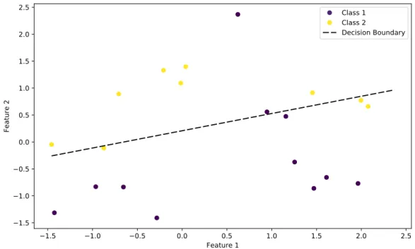
1.2 Linear model on simple binary classification dataset. . . 12

2.1 Neuron comparison. . . 17

(a) Biological . . . 17

(b) Artificial . . . 17

2.2 A simple neural network acceptingp-sized inputs, with one hidden layer consisting of two neurons. . . 18

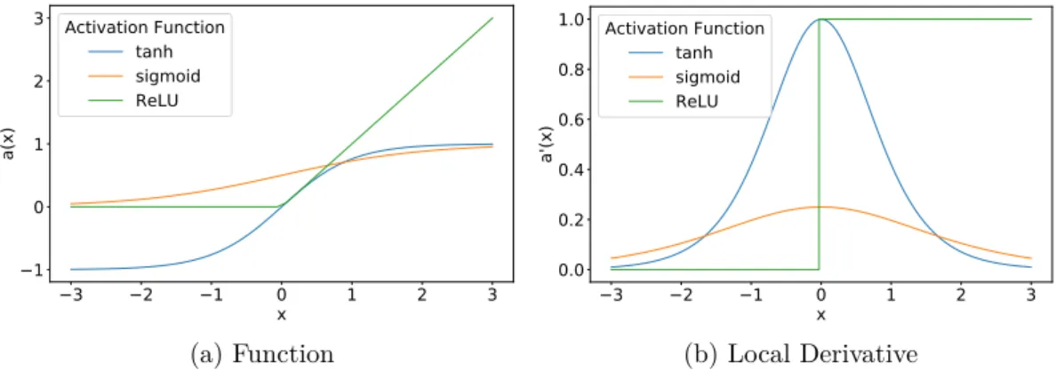
2.3 Activation functions. . . 20

(a) Function . . . 20

(b) Local Derivative . . . 20

2.4 Plots of the gradient descent example. (a) The training data points in input space. The shades in the background represent the class division in input space, with the decision boundary determined by least squares estimation. The dashed lines represent the gradient descent decision boundaries at different iterations. (b) The loss function at each iteration. . . 27

2.5 Simple dataset with two linearly inseparable classes. . . 34

2.6 Decision boundary of a single-layer neural network. . . 35

2.7 Decision boundary of a two-layer neural network. . . 35

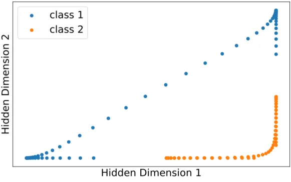
2.8 Hidden representation of a two-layer neural network. . . 36

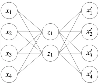
3.1 A simple single hidden layer autoencoder with four-dimensional inputs and with two neurons in the hidden layer. . . 40

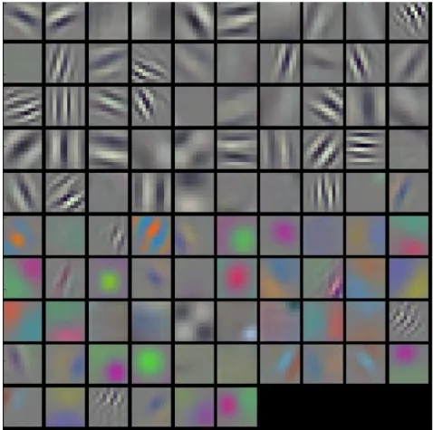
3.2 Visualising the first layer convolutional filters leared by a neural network in a large image dataset. . . 43

(12)

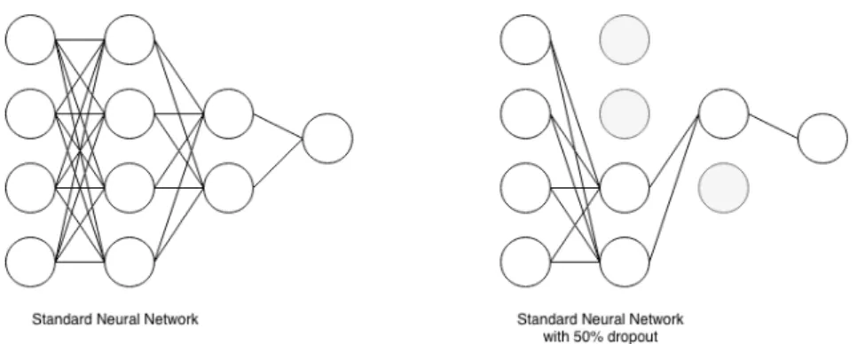
3.3 The effect that dropout has on connections between neurons. . . 46

3.4 An example of data augmentation for images. . . 47

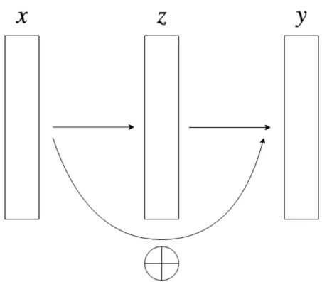
3.5 Diagram conceptualising a skip connection. . . 50

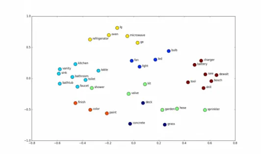
3.6 Learned word embeddings in a two-dimensional space. . . 51

3.7 Attention applied to image captioning. . . 52

3.8 Attention applied to machine translation. . . 53

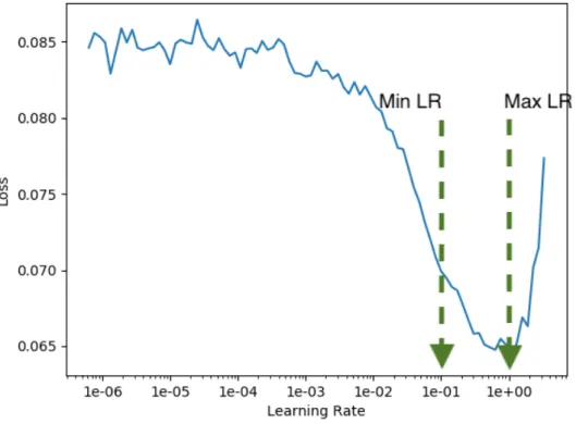
3.9 The learning rate schedule of the 1cycle policy. . . 56

3.10 An example output of a learning rate range test. . . 56

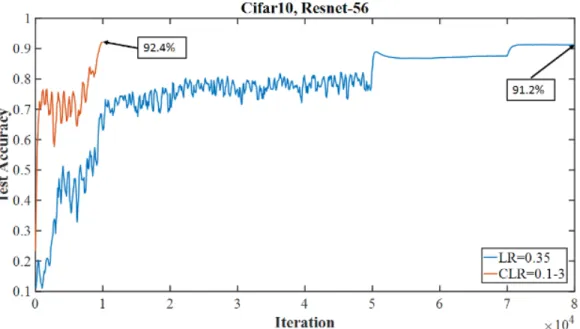
3.11 Reduced training iterations and improved performance facilitated by the super-convergence principle. . . 57

4.1 The effect of normalisation on continuous variables. . . 65

(a) Original . . . 65

(b) Gaussian Norm . . . 65

(c) Power Norm . . . 65

4.2 PCA of the ‘Education’ entity embedding weight matrix. . . 69

4.3 Combined representation of continuous and categorical features. . . 70

4.4 Illustration of the data points created by mixup augmentation. . . . 78

4.5 A display of the attention weights for a single observation in the dataset. . . 82

4.6 A permutation importance plot of an NN trained on the Adult dataset. 84 4.7 Feature importance values obtained from a boosted model trained on NN predictions. . . 84

4.8 Constant learning rate vs the 1cycle schedule. . . 86

4.9 A learning rate range test with different weight decays. . . 87

4.10 A full training run with different weight decays. . . 87

5.1 Kernel density estimation plots for each of the continuous features in the Adult dataset. . . 92

5.2 Bar plot for each of the categorical features in the Adult dataset. . 93

5.3 An example of an ROC curve related to one of the best models on the Adult dataset. . . 95

5.4 5-Fold Cross-validation dataset split schematic. . . 96

5.5 Effect of the embedding size if all categorical features are mapped to the same number of dimensions. . . 99

5.6 Effect of variable sizes on the performance of the NN model. . . 99

(13)

5.8 The average performance of ReLU and SeLU activation functions for shallow and deep networks as a function of the number of training epochs. . . 101 5.9 The average performance of ReLU and SeLU activation functions

for shallow and deep networks. . . 101 5.10 Average performance at each epoch for shallow and deep neural

networks, with and without skip connections. . . 102 5.11 Overall performance of the skip connections used in a shallow and

deep neural network. . . 102 5.12 Effect of the number of training samples on the performance of

neural networks. . . 103 5.13 Average performance of models using various mixup and weight

decay parameters. . . 104 5.14 Performance per epoch for models with different weight decays and

mixup ratios. . . 104 5.15 The effect of unsupervised pretraining on supervised classification

for tabular data. . . 105 A.1 Effect of the layer width and network depth on the performance on

the Adult dataset. . . 114 A.2 The effect of dropout on wide and narrow neural networks. . . 114

(14)

List of Tables

1.1 Preview of the Adult dataset. . . 4 4.1 Swap Noise Example. . . 77

(15)

List of Abbreviations and/or

Acronyms

ANN Artificial Neural Network AUC Area Under a Curve

CNN Convolutional Neural Network CTR Click-through Rate

CV Computer Vision DNN Deep Neural Network DL Deep Learning

GAN Generative Adversarial Network kNN k-Nearest Neighbour

mAP Mean Average Precision MI Multiple Imputations ML Machine Learning MLP Multi-layer Perceptron

NLP Natural Language Processing NN Neural Network

OLS Ordinary Least Squares RNN Recurrent Neural Network

(16)

ROC Receiver Operating Characteristic SGD Stochastic Gradient Descent SLT Statistical Learning Theory SotA State-of-the-Art

(17)

Notation

N number of observations in a dataset

p input dimension or the number of features for an observation K number of labels in a dataset

x p-dimensional input vector (x1, x2, . . . , xp)|

λ label

L complete set of labels in a dataset L={λ1, λ2, . . . , λK}

Y labelset associated with x, Y ⊆ L

ˆ

Y predicted labelset associated with x, ˆY ⊆ L

y K-dimensional label indicator vector, (y1, y2, . . . , yK)|,

associ-ated with observation x

(xi, Yi)Ni=1 multi-label dataset with N observations

D dataset

h(·) multi-label classifier h:_Rp _→₂L_{, where} _h₍_x_{) returns the set of} labels for x

θ set of parameters for h(·) ˆ

θ set of parameters for h(·) that optimise the loss function L(·,·) loss function between predicted and true labels

f(·) label prediction module, f :_Rp _→

RK t(·) thresholding function, t :_RK _{→ {}₀_,₁_}K

N(x) points in the input space neighbourhood of x

(18)

Chapter 1

Introduction

1.1

Deep Learning

This thesis is concerned with the study of deep learning approaches to solve

machine learning (ML) tasks. More specifically, our interest lies in machine learning tasks that may be solved using tabular data inputs. The deep learning field is an extention of the class of machine learning algorithms calledArtificial Neural Networks (NNs). Whereas until relatively recently, the neural network field was not an over-active research field, rapid development in computing power and the growing abundance of data lead to advances in neural network optimisation and architecture. These advances constitutes the deep learning field as we know it today (Lecun et al., 2015).

Currently, deep learning is receiving a remarkable amount of attention, both in research and in practice (see Figure 1.1). Much of the deep learning hype stems from the tremendous value neural networks have shown in application areas such as computer vision (Huet al., 2017), audio processing (Battenberg

et al., 2017), and natural language processing (NLP) (Devlin et al., 2018). In these application areas, deep learning methods have reached a maturity level sufficient to be able to run these systems in a production or commercial environment. Examples of the application of deep learning in commercial applications include voice assistants like Amazon Alexa (Sarikaya, 2017), face recognition with Apple iPhones 1_{, and language translation with Google (Wu}

et al., 2016).

1_{https://www.apple.com/business/site/docs/FaceID_Security_Guide.pdf} 2_{https://trends.google.com/trends/}

3_{https://www.semanticscholar.org/}

(19)

2010 2011 2012 2013 2014 2015 2016 2017 2018 Year

Number of hits (normalised)

Deep Learning Trends

Semantic Scholar Google Trends

Figure 1.1: The exponential growth of published papers and Google search terms containing the term Deep Learning. Sources: Google Trends2_{, Semantic}

Scholar3

One of the most attractive attributes of deep learning is its ability to model almost any input-output relationship. This has lead to the use of deep learning in a very wide array of applications.

For example, deep learning has been used to generate art (Gatys et al., 2015) and music (Mogren, 2016), to control various modules in autonomous cars (Fridman et al., 2017), to play video games (Mnih et al., 2013), to recommend movies (Covington et al., 2016), to improve the quality of images (Shi et al., 2016), and to beat the world’s best Go player (Silver et al., 2017).

A common characteristic of all of the above deep learning applications is that the data used to construct them contain the same type of values or measurements. That is, in computer vision the data represent pixel values, whereas in NLP and in audio processing the data represent words and sound waves. This is not a criterion for deep learning algorithms to be successful, but may be viewed as a driver for their success in these application domains. It is simpler to model data consisting of the same type of measurements, since each input feature may be treated the same. Furthermore in the above deep learning applications, it is found that in each of these domains, universal patterns exist.

(20)

This allows for knowledge to be transferred between tasks belonging to the same domain. The knowledge to be transferred is both the knowledge aquired by humans, and the knowledge acquired by a deep learning model. For example, in computer vision, advances in classifying pictures of pets will most likely also facilitate improved identification of tumors in X-rays. That is, patterns learned by a deep learning model when attempting one task, may also be useful in a different, but related task. This phenomenon constitutes a second reason for the successful application of deep learning methods, and is studied in the field of transfer learning.

A data domain in which deep learning have not yet been very successful, is that of tabular data. Atabular dataset can be represented by a two-dimensional table, where each of the rows of the table corresponds to one observation and where each column denotes an individual meaningful feature. We further explain the use of tabular data in Section 1.2 below.

Some research have recently been done on the use of deep learning models for tabular data. See for example Shavitt and Segal (2018) and Song et al. (2018). However, state-of-the-Art (SotA) results are reported only rarely (de Brébisson

et al., 2015), and in the Kaggle competition found at the following website4_).

Therefore it can be said that the area is nowhere near as mature or receiving as much attention as is the case with deep learning for computer vision or for NLP. In a comprehensive study in the paper by Fernández-Delgadoet al.(2014), it was found that ML tasks that make use of tabular data are typically more effectively solved using tree-based methods. This is also evident when one considers the winning solutions of relevant Kaggle competitions5. A possible explanation for the superior performance of tree-based metods, is the heterogeneity of tabular data (Shavitt and Segal, 2018), which forms part of the discussion in the next section.

1.2

Tabular Data

In this section we make use of the so-called Adult6 _{dataset in order to discuss}

the use of tabular data. The reader may refer to Table 1.1 for an excerpt of this dataset. Note that the data were collected during an American census

4_{https://www.kaggle.com/c/porto-seguro-safe-driver-prediction/discussion/44629} 5_{https://www.kaggle.com}

(21)

where the aim was to predict whether or not an indivdual earns more than $50,000 a year.

age occupation education race sex >=50k

1 49 Assoc-acdm White Female 1

2 44 Exec-managerial Masters White Male 1

3 38 HS-grad Black Female 0

4 38 Prof-specialty Prof-school Asian-Pac-Islander Male 1 5 42 Other-service 7th-8th Black Female 0 6 20 Handlers-cleaners HS-grad White Male 0

Table 1.1: Preview of the Adult dataset.

Table 1.1 represents a typical tabular dataset, where the columns contain measurements on different features. Therefore different columns may contain different data types: some columns may consist of continuous measurements, whereas other columns may contain discrete or categorical measurements. Furthermore, in tabular data, the rows and columns occur in no particular order. This of course stands in contrast to image or text data.

Many important ML applications make use of tabular data. Some of these applications are listed below:

• Various tasks that make use of Electronic Health Records. These include the prediction of in-hospital mortality rates, and of prolonged length of stay (Rajkomar et al., 2018);

• Recommender systems for items like videos (Covington et al., 2016) or property listings (Haldar et al., 2018);

• Click-through rate (CTR) prediction in web applications, i.e. predicting which item a user will click on next (Songet al., 2018);

• Predicting which clients are at risk of defaulting on their accounts7; • Predicting store sales (Guo and Berkhahn, 2016); and

• Drug discovery (Klambauer et al., 2017).

Tabular datasets take on various shapes and sizes: the number of rows may range from hundreds to millions, and the number of columns also has no limits. Other complicating characteristics of tabular datasets include: - That it is not unusual for tabular datasets to be noisy; - That a proportion of the

(22)

observations may have missing features and/or incorrect values; and - That continuous measurements may be based upon vastly different scales, some even containing outliers, whereas categorical features may have high cardinality which in turn leads to sparse data.

During the construction of models for tabular datasets, the most important step in terms seeking improvements in model performance, is pre-processing and manipulation of the input features (Rajkomar et al., 2018). This includes data merging, customising, filtering and cleaning. In a process called feature engineering, one strives to create new features from the original features based on some domain knowledge. The idea is that such engineered features enables a model to learn interactions between features, thereby facilitating more accurate prediction. Feature engineering is an extremely laborious process with no clear recipe to follow and therefore typically cannot succesfully be implemented without some domain expertise.

Ensemble methods based upon trees are currently viewed as the most effective machine learning models for tabular datasets. As mentioned above, a possible reason for this may be their robustness to different feature scales and data types, linked with their ability to effectively model interactions among features with different data types.

Indeed, in the context of tabular data, classical neural network approaches are no match for tree ensembles. Although the deep learning field has advanced and matured a lot in recent years, it is not yet clear how to leverage these modern techniques to effectively build and train deep neural networks (DNNs) on tabular datasets. In this thesis we explore ways of doing so. By reviewing the most recent literature on the topic, and through empirical work, we aim to summarise best practices when using deep learning for tabular data.

1.3

Challenges of Deep Learning for Tabular

Data

Some of the challenges of deep learning for tabular data have been alluded to in earlier sections of this chapter. These will form the framework for our literature review later on. Therefore, some of the important questions to ask when applying deep learning for tabular data (which relates to these challenges), are summarised below.

(23)

• How should input features be represented numerically? We have mentioned that tabular data consist of mixed feature data types, i.e. a combination of categorical and continuous features. The question here relates to how these heterogeneous features should be processed and presented to the model during training.

• How can we exploit feature interactions? Once we have found the optimal feature representation for all feature data types, we will need a way to effectively learn the interactions among them, and also a way to learn how they relate to the target. This is a crucial step towards the effective application of deep learning models to tabular data.

• How can we be more sample efficient? Tabular datasets are typically smaller than datasets used in computer vision and in NLP. Moreover, no general large dataset with universal properties exists to be used by a model to learn from (as is the case in for example in transfer learning for image classification). Thus, a key challenge is to facilitate learning from less data.

• How do we interpret model decisions? The use of deep learning is often restricted by its perceived lack of interpretability. Therefore we need ways of explaining the model output in order for it to be useful in a wider array of applications.

Clearly there are several considerations when it comes to using deep learning for tabular data. The main objective of this thesis is to find the best ways of answering the above questions. Towards this objective, the study should lead to a thorough understanding of the status quo of the field, and of the necessary factors in order to ensure deep learning to be as effective in other data domains as it currently is in fields such as computer vision and NLP.

The study is divided in two parts. We start by first providing an overview of the relevant literature. Subsequently, we make use of experimental work in order to compare various deep learning algorithms (and possible improvements) on relevant datasets. Here an important aim will be to ensure our experiments to be rigorous. The importance of rigorous research has relatively recently again been emphasised during an NIPS talk8, during which researchers in the deep learning field have been criticised for the growing gap between the understanding of its techniques, and practical successes. Currently much

(24)

more emphasis is placed on the latter. The speakers urged the deep learning community to be more rigorous in their experiments where, for them, the most important part of rigor is better empiricism, not more mathematical theories. Better empiricism in classification may include, for example, practices such as using cross-validation to estimate the generalisation ability of a model, and reporting standard errors. Empirical studies should involve more than simply attempting to beat the benchmark. For example, where possible, they should also involve simple experiments that facilitate understanding why some algorithms are successful, while others are not.

In addition, we want the empirical work in this study to be as reproducible as possible. This aspect is often overlooked. However, it is a crucial aspect, ensuring transparent and accountable reporting of results. Reproducibility add to the value of research, since without it, researchers are not able to build on each other’s work. Hence all code, data and necessary documentation in order to reproduce the experiments done in this study are available 9_.

Having stated the objectives of this study, we now turn to a discussion of the fundamental concepts of Statistical Learning Theory. This is followed by a more detailed overview of the thesis.

1.4

Overview of Statistical Learning Theory

Machine- or statistical learning algorithms (here used interchangeably) are used to perform certain tasks that are too difficult to solve with fixed rule-based programs. Hence, statistical learning algorithms are able to use data in order to learn how to perform difficult tasks. For an algorithm to learn from data means that it can improve its ability to perform an assigned task with respect to some performance measure, by processing data. In this section we discuss some of the important types of tasks, data and performance measures in the statistical learning field.

A learning task describes the way in which an algorithm should process an observation. An observation is a collection of features that have been measured, corresponding to some object or event that we want the system to process, for example an image. We will represent an observation by a vector x∈_Rp_,

where each element xj of the vector is an observed value of the j-th feature,

(25)

j = 1, . . . , p. For example, the features of an image are usually the color intensity values of the pixels in the image.

Many kinds of tasks can be solved using statistical learning. One of the most common learning tasks is that of classification, where it is expected of an algorithm to determine which of K categories an input belongs to. In order to complete the classification task, the learning algorithm is usually asked to produce a function f : _Rp _{→ {}₁_{, . . . , K}_}_{. When} _y₌ _f₍_x_{), the model assigns}

an input described by the vector xto a category identified by the numeric code y, called theoutput or response. In other variants of the classification task, f may output a probability distribution over the possible classes.

Regression is another main learning task and requires the algorithm to predict a continuous value given some input. This task requires a function f :_Rp _→

R, where the only difference between regression and classification is the format of the output.

Learning algorithms learns such tasks by observing a relevant set of data points. A dataset containing N observations ofpfeatures is commonly denoted by a data matrix X :N ×p, where each row represents a different observation and where each column corresponds to a different feature of the observations,

i.e. X =         x11 x12 . . . x1p x21 x22 . . . x2p .. . ... . .. ... xN1 xN2 . . . xN p         .

Often the dataset includes annotations for each observation in the form of a label (i.e. in classification) or in the form of a target value (i.e. in regression). These N annotations are represented by the vector y, where the element yi

is associated with the i-th row of X. Therefore the response vector may be denoted by y=         y1 y2 .. . yN         .

Note that in the case of multiple labels or targets, a matrix representation Y :N ×K is required.

(26)

Statistical learning algorithms can be divided into two main categories,

viz. supervised and unsupervised algorithms. This categorisation is determined by the presence (or absence) of annotations in the dataset to be analysed. Unsupervised learning algorithms learn from data consisting only of features, X, and are used to find useful properties and structure in the dataset (see Hastie et al., 2009, Ch. 14). On the other hand, supervised learning algorithms learn from datasets which consist of both features and annotations, (X, Y), with the aim to model the relationship between them. Therefore, both classification and regression are considered to be supervised learning tasks.

In order to evaluate the ability of a learning algorithm to perform its assigned task, we have to construct a quantitative performance measure. For example, in a classification task we are usually interested in the accuracy of the algorithm, i.e. the percentage of times that the algorithm assigns the correct classification. We are mostly interested in how well the learning algorithm performs on data that it has not seen before, since this demonstrates how well it will perform in real-world situations. Thus, we typically evaluate the algorithm on a test set of data points. This dataset is independent of the training set of data points that was used during the learning process.

For a more concrete example of supervised learning, and keeping in mind that the linear model is one of the main building blocks of neural networks, consider the learning task underlying linear regression. The objective here is to construct a system which takes a vector x∈_Rp _{as input and which predicts}

the value of a scalar y ∈ _R as response. In the case of linear regression, we assume the output to be a linear function of the input. Let ˆy be the predicted response. We define the output to be

ˆ

y= ˆw|x,

where ˆw = [w0, w1, . . . , wp] denotes a vector of parameters and where x =

[1, x1, x2, . . . , xp]. Note that an intercept is included in the model (also known

as a bias in machine learning). The parameters are values that control the behaviour of the system. We can think of them as a set of weights that determine how each feature affects the prediction. Hence the learning task can be defined as predicting y from xthrough ˆy= ˆw|_x_.

We of course need to define a performance measure to evaluate the linear predictions. For a set of observations, an evaluation metric tells us how (dis)similar the predicted output is to the actual response values. A very

(27)

common measure of performance in regression is themean squared error (MSE), given by M SE = 1 N N X i=1 (yi−yˆi)2.

The process of learning from data (or fitting a model to a dataset) can be reduced to the following optimisation problem: find the set of weights, ˆw, which produces a ˆy that minimises the MSE. Of course this problem has a closed form solution and can quite trivially be found by means of ordinary least squares (OLS) (see Hastie et al., 2009, p. 12). However, we have mentioned that we are more interested in the algorithm’s performance evaluated on a test set. Unfortunately the least squares solution does not guarantee the solution to be optimal in terms of the MSE on a test set, rendering statistical learning to be much more than a pure optimisation problem.

The ability of a model to perform well on previously unobserved inputs is referred to as itsgeneralisation ability. To be able to fit a model that generalises well to new unseen data cases is the key challenge of statistical learning. One way of improving the generalisation ability of a linear regression model is to modify the optimisation criterionJ, to include aweight decay (orregularisation) term. That is, we want to minimise

J(w) = M SEtrain+λw|w,

whereJ(w) now expresses preference for smaller weights. The parameterλ is non-negative and needs to be specified ahead of time. It controls the strength of the preference by determining how much influence the penalty term, w|_w_, has on the optimisation criterion. If λ = 0, no preference is imposed, and the solution is equivalent to the OLS solution. Larger values of λ force the weights to decrease, and thus referred to as a so-calledshrinkage method ((cf. for example Hastie et al., 2009, pp. 61-79) and (Goodfellow et al., 2016).

We may further generalise linear regression to the classification scenario. First, it is important to note the different types of classification schemes. Consider G, the discrete set of values which may be assumed byG, whereG is used to denote a categorical output variable (instead of Y). Let |G| = K denote the number of discrete categories in the set G. The simplest form of classification is known as binary classification and refers to scenarios where the input is associated with only one of two possible classes, i.e. K = 2.

(28)

When K > 2, the task is known as multiclass classification. In contrast, in

multi-label classification an input may be associated with multiple classes (out of K available classes), where the number of classes that each observation belongs to, is unknown. In the remainder of this section, we introduce the two single label classification setups, viz. binary and multiclass classification.

In multiclass classification, given the input values X, we would like to accurately predict the output, G, where our prediction is denoted by ˆG. One approach would be to represent G by an indicator vector YG : K ×1, with

all elements zero except in the G-th position, where it is assigned a 1. That is, Yk = 1 for k = G and Yk = 0 for k 6= G, k = 1,2, ..., K. We may

then treat each of the elements in YG as quantitative outputs, and predict

values for them, denoted by ˆY = [ ˆY1, . . . ,YˆK]. The class with the highest

predicted value will then be the final categorical prediction of the classifer, i.e.

ˆ

G= arg maxk∈{1,...,K}Yˆk.

Within the above framework we therefore seek a function of the inputs which is able to produce accurate predictions of the class scores,i.e.

ˆ

Yk= ˆfk(X),

for k = 1, . . . , K. Here ˆfk is an estimate of the true function, fk, which is

meant to capture the relationship between the inputs and output of class k. As with the linear regression case described above, we may use a linear model ˆfk(X) = ˆwk|X to approximate the true function. The linear model for

classification partitions the input space into a collection of regions labelled according to the predicted classification, where regions are created by linear

decision boundaries (see Figure 1.2 for an illustration). The decision boundary between classes k andl is the set of points for which ˆfk(x) = ˆfl(x). These set

of points form an affine set or hyperplane in the input space.

After the weights are estimated from the data, an observation represented by x(including the unit element) may be classified as follows:

• Compute ˆfk(x) = ˆw|kxfor k = 1, . . . , K.

• Identify the largest component and classify to the corresponding class,

i.e. Gˆ = arg maxk∈{1,...,K}fˆk(x).

One may view the predicted class scores as estimates of the conditional class probabilities (or posterior probabilities), i.e. P(G=k|X =x)≈fˆk(x).

(29)

1.5 1.0 0.5 0.0 0.5 1.0 1.5 2.0 2.5 Feature 1 1.5 1.0 0.5 0.0 0.5 1.0 1.5 2.0 2.5 Feature 2 Class 1 Class 2 Decision Boundary

Figure 1.2: Linear model on simple binary classification dataset.

Although the values sum to 1, they do not lie in the interval [0,1]. A way to overcome this problem is to estimate posterior probabilities using the logit transform of ˆfk(x). That is,

P(G=k|X =x)≈ e ˆ fk(x) PK l=1e ˆ fl(x).

Through this transformation, the estimates of the posterior probabilities sum to 1 and are contained in [0,1]. The above model is the well-known logistic regression model (Hastie et al., 2009, p. 119). With this formulation there is no closed form solution for the weights. Instead, the weight estimates may be searched for by maximising the log-likelihood function. One way of doing this is by minimising the negative log-likelihood using gradient descent, which will be discussed in the next chapter.

Finally in this section, note that any supervised learning problem can also be viewed as a function approximation problem. Suppose we are trying to predict a variable Y given an input vector X, where we assume the true relationship between them to be given by

Y =f(X) +,

whererepresents the part of Y that is not predictable fromX, because of, for example, incomplete features or noise present in the labels. Then in function

(30)

approximation we are estimating f by ˆf. In parametric function approximation, for example in linear regression, estimation off(X, θ) is equivalent to estimating the optimal set of weights, ˆθ. In the remainder of the thesis, we refer to ˆf as the model,classifier or learner.

1.5

Outline

This chapter provided the context and some theoretical background for this study. An outline of the remainder of the thesis follows below:

In Chapter 2, the theory underlying neural networks is described. The building blocks of neural networks are discussed, thereby introducing neurons, basic layers and the way in which neural networks are trained. The important concept of regularisation is also discussed. Using the perspective of represent-ation learning, we then attempt to gain insight into what happens inside a neural network.

Chapter 3 continues the discussion by focusing on the key advances in neural networks in recent times. The idea is that all concepts introduced in this chapter should potentially be able to facilitate the construction of improved deep neural networks on tabular data. Improved ways of preventing overfitting, such as data augmentation, the use of dropout and transfer learning, as well as the SotA training policy called 1cycle are analysed here. New developments in architectural design are also highlighted. The chapter concludes with approaches towards interpreting neural networks and their predictions.

Chapter 4 may be viewed as a core chapter of the thesis. It mainly serves as a literature review of all research with regard to deep learning for tabular data. The chapter is organised according to the modelling challenges faced when using deep learning for tabular data, investigating and comparing what other researchers have done in order to overcome these challenges. It will be seen that the key concept involves finding the right representation for tabular data. This may be done through embeddings, and by means of designing architectures that can efficiently learn feature interactions. This is for example done with attention models, possibly with the help of unsupervised pretraining.

In Chapter 5 we empirically investigate several claims made in the literature. The aim of the chapter is to evaluate and compare different approaches towards tackling the various challenges. Hence the main experiments involve evaluating neural networks at various samples sizes, evaluating potential gains from

(31)

doing unsupervised pretraining and using data augmentation, and comparing attention modules with classic fully-connected layers. We also make use of permutation importance and knowledge distillation in order to illustrate a way in which neural networks may be interpreted.

The thesis concludes in Chapter 6, where we summarise our work, some highlights and the main take-home points. The limitations of this study are discussed, and promising future research directions identified.

(32)

Chapter 2

Neural Networks

2.1

Introduction

Not unlike most supervised machine learning models, an artificial neural network is a function which maps inputs to outputs, i.e. f :x→y. The structure of f is often loosely compared to the structure of the human brain. Oversimplified, the brain consists of a collection of interconnected neurons. Each neuron can generate and receive signals. A received signal may be described as an input to a neuron, whereas a sent signal may be described as an output from that neuron. If two neurons are connected, it means that the output from the one neuron serves as input to the other. In a very simple model of the brain, one may argue that a neuron receives several signals, which it weighs and combines, and if the combined value of the inputs is higher than a certain threshold, the neuron sends an output signal to the next neuron. Figure 2.1 (a) provides a schematic of a biological neuron1_.

An artifical neural network tries to mimic this model of the human brain: it is set up to consist of several layers of connected units (or neurons). With exception of units in the first and final layers, each unit outputs a weighted combination of its inputs, combined with a simple non-linear transformation. In each layer of the neural network, the input is passed through each of the neurons. In turn, their output is passed to the next layer.

The transformation at each neuron is controlled by a set of parameters, also known as weights. Training a neural network involves tuning these weights in order to obtain some desired output. During training, the neural network

1_{Image credit: https://www.jeremyjordan.me/intro-to-neural-networks/}

(33)

receives as input a set of training data. The neural network weights are then learned in such a way that, when given a new set of inputs, the output predicted by the neural network matches the corresponding response of interest as closely as possible. The process of using the training data to tweak the weights is done by means of an optimisation algorithm called Stochastic Gradient Descent (SGD).

Although recently there has been plenty of excitement around advances in neural networks, it is well known that they were invented many years ago. The development of neural networks dates back at least as far as the invention of perceptrons in Rosenblatt (1962). It is also interesting to compare modern neural networks with the Projection Pursuit Regression algorithm in statistics (Friedman and Stuetzle, 1981). Only recently a series of breakthroughs caused neural networks to become more effective, leading to the renewed interest in the field.

The aim of this chapter is to provide an overview of neural networks, emphasising their basic structure §2.2 and the way in which they are trained §2.3. This is done with a view to discuss modern neural network structures and training policies in Chapter 3, which in turn will help us shed light on Deep Learning for tabular data. In §2.4 and §2.5, regularisation for neural networks and the use of adaptive learning rates are discussed. These are necessary components for regulating the generalisation performance of NNs, as well as for keeping the required training time at bay. The chapter concludes with a section on representation learning §2.6, which is an important topic toward understanding the inner workings of neural networks.

2.2

The Structure of a Neural Network

2.2.1

Neurons and Layers

In basic terms, a neural network processes an input xby sending it through a series of layers. The neurons in each layer apply some transformation to their inputs, resulting in a set of outputs which are again passed on to the next layer of neurons. Eventually, the final layer produces the neural network output. In this section we provide more detail regarding the neural network structure. We start with a description of the operations inside each neuron, followed by a discussion of the way in which the neurons may be connected in layers in order

(34)

to form a complete neural network structure. Our discussion is based upon a simple regression example.

Suppose we are in pursuit of a function which is able to estimate some continuous target, y, given ap-dimensional inputx,e.g. estimating the taxi fare from features such as distance travelled, time elapsed and number of passengers. A single neuron may act as such a function. It modelsyby computing a weighted average of the input features. This operation is illustrated in Figure 2.1 (b).

(a) Biological (b) Artificial

Figure 2.1: Neuron comparison. In equation form, this function may be written as

w1 ·x1 +w2·x2+· · ·+wp·xp+b =y,

where{wk}pk=1, are the weights applied to each of the inputs{xk}pk=1 and where

b denotes the constant bias term. Clearly, this equation is simply the very common linear model and thus also can be written as

w|x+b =y,

where x = [x1 x2 . . . xp]| represents the input, and where resepctively

w = [w1 w2 . . . wp]| and y denote the weights and output. We may

of course compress the above equation to w|_x ₌ _y_{, where} _w _{is amended} to include the bias term, and where x is amended to include a 1, i.e. x = [1 x1 . . . xp]| is the input, and w = [b w1 . . . wp]| is the weight

vector.

The weights convey the importance of each input feature in predicting the target. Larger values of |wk| indicate greater contributions of xk toward the

output. If wk = 0, xk has no influence on the target. However the weights are

(35)

As discussed in Chapter 1, in linear regression this is done by means of OLS. However, since a neural network consists of many inter-conncected neurons, an alternative estimation procedure is required. This is the topic of the next section.

Often a linear model will be too rigid to model a certain response of interest. In order to fit a more flexible model, we may add more neurons. Consider the use of two neurons, z1 and z2, where the second neuron (z2) accepts the same input as the first neuron (z1), but uses a different set of weights. Thus, we have two different outputs produced by the two neurons, i.e. z1 = w1|x and

z2 =w2|x. In order to produce a final estimate from the initial two estimates,

viz. z1 and z2, they are passed to a third neuron. That is, y = w3|z, where

z = [z1 z2]|. Figure 2.2 illustrates this pipepline in network form.

Figure 2.2: A simple neural network accepting p-sized inputs, with one hidden layer consisting of two neurons.

The first two neurons each received allp inputs and each produced a single output. These two outputs were received by the third neuron, and combined in order to produce the final output, viz. y. The operations performed byz1 and z2 may be expressed as z =Wx|_{, where}

W =   w₁| w₂|  =   w10 w11 w12 . . . w1p w20 w21 w22 . . . w2p   and z = [z₁ z₂]|.

The collection of z1 and z2 is called a layer. Since our third neuron (which is also a layer but with a single neuron) receives the output of this layer as input, it is possible to express the complete input-output relationship in one equation, i.e.

(36)

Note here that the weights from the first layer, viz. W, and the weights from the third neuron, viz. w3, may be collapsed into a single vector w,

effectively reducing all of the neuron operations to a single neuron representation. Therefore the fitted model is still linear. In order to fit a non-linear model, a non-linear transformation function has to be applied to the output of each layer. This function is called an activation function.

Incorporating an activation function, the neural network equation may be written as

y=a2(w|3a1(Wx)),

wherea1 denotes the activation function applied after the first (linear) layer,

and where a2 denotes the activation function applied after the final layer.

The introduction of non-linear activation functions serves to enlarge the class of functions that can be approximated by the network. That is, activiation functions enable the network to learn complex non-linear relationships between inputs and outputs. Next, we briefly discuss various activation functions.

2.2.2

Activation Functions

Since any simple non-linear and differentiable function can be used as activation function, there are plenty of activation functions to choose from. Originally, the sigmoid activation function, viz. sigmoid(x) = ₁₊1_e−x, was a common choice

(Rumelhart et al., 1988). The S-shape of the sigmoid activation function, and its range between 0 an 1 is illustrated in Figure 2.3 (a). Note that the reason why the sigmoid function fell out of favour in terms of its use as activation function in neural networks is because of issues related to the gradient based optimisation procedure of NNs. For example, gradient weight updates that veer to far in different directions are caused by the values of sigmoid activations that are not centered around zero. Some other issues with the sigmoid activiation function are discussed in more detail in Section 2.3.

The hyperbolic tangent or tanh activation function, on the other hand, does return outputs centered around zero. It takes the form tanh(x) = e_exx−₊e_e−−xx

and its shape is illustrated in Figure 2.3 (a). However, the problem with both the sigmoid and tanh activation functions is that they may lead to saturated gradients during training. To see this, consider the tails of the sigmoid and tanh functions, which indicate that the gradients of both these functions tend to zero as |x| → ∞. During training, this may cause weight updates to be nearly

(37)

3 2 1 0 1 2 3 x 1 0 1 2 3 a(x) Activation Function tanh sigmoid ReLU (a) Function 3 2 1 0 1 2 3 x 0.0 0.2 0.4 0.6 0.8 1.0 a'(x) Activation Function tanh sigmoid ReLU (b) Local Derivative

Figure 2.3: Activation functions.

zero, resulting in the network getting stuck at a certain point in the parameter space. Furthermore, the maximum gradient of the sigmoid activation function turns out to be only 0.25 (at x= 0.5). The nature of the chain rule therefore causes lower layers in the network to train much slower than higher layers. The tanh activation function typically have larger derivatives than the sigmoid function. Thus, it is not as susceptible to this vanishing gradient problem. However, it is still not immune to it. The local derivatives of the activation functions discussed in this section are illustrated in Figure 2.3 (b). The form of these functions will become more apparent in Section 2.3.

To date, the most popular choice in activation function is the Rectified Linear Units (ReLU) non-linearity. It is defined as:

relu(x) =      x if x >0 0 otherwise .

The shape of the ReLU activiation and of its derivative are illustrated in Figure 2.3 (a) and (b), respectively. Use of the ReLU alleviates the gradient vanishing problem as the derivative of this function is always 1 (for positive x values). This results in significantly shorter steps to convergence, as found by the authors in (Krizhevsky et al., 2012). However, ReLUs may suffer from the “dead ReLU” problem, which is, if a ReLU neuron is assigned a zero weight,

its weights receive zero gradients. In this way, neurons may be “clamped to zero” and may remain permanently “dead” during training. This sparsity of the activations is what some believe is the reason for the effectiveness of ReLUs (Sunet al., 2014). If dead activations needs to be avoided, alternative activation functions to apply include PReLUs (He et al., 2015a) and Leaky ReLUs (Maas

(38)

et al., 2013).

Selecting an appropriate activation function for a specific task typically involves a trial-and-error process. For general tasks, the use of ReLUs after each linear layer may suffice and has to some extent become standard practice. In the context of classification, for each class, it is often useful to produce outputs between 0 and 1 as estimates of conditional class probabilities. Therefore one often uses a sigmoid activation function on the output layer for a binary classification task. In the context of (single label) multiclass classifcation, it is also desirable for these ouputs to sum to 1, therefore in this case, an activation function called softmax is typically used. Note that the softmax activation,viz.

softmax(x)k = e xk

PK

l=1xl

is simply the logit transformation introduced in §1.4. In a regression context, we mostly omit the use of an activation function on the output layer.

In our empirical work, we will experiment with the use of the different activation functions discussed in this section, and compare their performance to that of Scaled Exponential Linear Units (SELUs) (Klambauer et al., 2017), where the latter is supposed to facilitate more effective training of deeper neural networks. Note that the depth of a neural network refers to its number of hidden layers, whereas the width of a layer refers to the number of neurons it consists of. Selecting network depth and layer width is the topic of the next section.

2.2.3

Size of the Network

The network depth and the width of its hidden layers (i.e. the size of the network) are hyperparameters of the model. They control the ability of a neural network to model complex functions, which is also often referred to as its flexibility. In statistical learning it is well known that increasing the flexibility of a model is typically only beneficial up to a certain point, whereafter a further increase in flexibility will be detrimental to its prediction performance on new unseen data cases. Suboptimal test performance due to a too flexible model is known as overfitting. Appropriate selection of the flexibility of the model is also important in the case of neural networks. The challenge is to find a network size which is large enough to capture all the complexities in the data, but small enough to avoid overfitting. In addition, whereas more layers facilitate a more flexible fit, larger networks require more time and more hardware capacity in

(39)

order to train them.

Currently the best way of finding the optimal size of a network for a given problem is by means of experimentation. Note therefore that for many of the components of neural networks in deep learning, hyperparameter values are selected through a process of trial-and-error. Whereas appropriate specification of the size of a neural network is certainly important, in §2.4, we will see why tuning the size of a network is not necessarily the best way to control overfitting.

Theoretically, according to the universal approximation theorem (Cybenko, 1989), a neural network with a single hidden layer and with a finite number of neurons can approximate any continuous function. This begs the question: why are additional hidden layers required? As stated in Ba and Caurana (2013), although a neural network can represent any function, it does not mean that the available learning algorithm is able to find these optimal weights. Moreover, it may be the case that the number of neurons needed in order for a single hidden layer network to represent a specific function of interest, is infeasibly large. By choosing deeper networks we are assuming that the function we are trying to learn is composed of several simpler functions. Incorporating this prior belief has empirically been shown to be useful (Goodfellow et al., 2016, pp.197-198). This is especially true in the case of tasks that may be partitioned into smaller subtasks, for example in computer vision.

In our empirical work we investigate the effect of network depth and layer width on the generalisation performance of neural networks. We also analyse why networks used in the case of tabular data are typically much shallower than in the case of computer vision or NLP applications. For some additional insight in the matter, later on in this chapter we view the problem of the specification of the network size from a representation learning perspective.

Note, that there also exists other classes of neural networks besides the basic feed-forward network focussed on thus far. The convolutional neural network (CNN) is a very common choice in computer vision (Krizhevskyet al., 2012) and only recently in NLP applications (Devlin et al., 2018). Its main difference to standard NNs is the use of a convolutional layer that performs a cross-correlation operation on its inputs with a set of learnable filters. The

recurrent neural network (RNN) (Mikolov et al., 2010) is a class of neural networks that are helpful for modelling variable length inputs or outputs, for example in machine translation or video classification. A RNN has loops in

(40)

them, allowing information to persist. It can also be thought of as multiple copies of the same network, each passing a message to its successor, if one were to “unfold” the loops. These classes of neural networks are not within the scope of this work since they have no clear benefit for using with tabular data.

2.3

Training a Neural Network

Briefly, basic training of a neural network entails the following four steps: 1. Initialisation: random numbers are assigned to the network parameters. 2. Forward propagation: the input is passed through the network layers in

order to produce an output.

3. Error calculation: the predicted output is compared to the true output, and the difference measured by means of an appropriate objective function. 4. Backward propagation: the gradients of the objective function with

respect to the weights are obtained, and the network weights are updated accordingly.

The above steps are typically repeated until the loss function is found to converge. Note however that convergence may require many training epochs. The following four subsections are each devoted to a discussion of one of the aforementioned steps.

2.3.1

Weight Initialisation

Taining a neural network starts with a weight initialisation step. A poorly initialised network hampers the training procedure: it increases the number of iterations needed, reduces the quality of the local optima found and makes convergence more difficult. In order to think about sensible initialisation, first note that we expect the number of positive and negative weights of a well trained neural network to be equal. If we initialise all weights to be zero, each neuron will compute the same output. Consequently, each neuron will produce the same gradient and undergo the same weight update. Hence we want to initialise the weights as small as possible, but each weight should be unique. Sampling the initial weights from the standard normal distribution seems to be a natural choice. However it turns out that the variance of the outputs from randomly initialised neurons grows as the number of inputs increase. Therefore

(41)

an option is to scale the weight vector generated from the standard normal distribution by the square root of its number of inputs. Such a scaling step will normalise the variance of the output, ensuring that all neurons in the network initially have approximately the same output distribution. In addition, it serves to improve the rate of convergence when training the network.

Very deep neural networks have difficulties to converge when using the above mentioned initialisation (Simonyan and Zisserman, 2014). He et al. (2015b) propose an alternative initialisation, which was made specifically in the context of using ReLU activation functions and making it easier to train deep neural networks.

2.3.2

Optimisation

We have briefly seen in Chapter 1 that there is a connection between statistical learning and optimisation. Optimisation refers to the task of altering xin order to either minimise or maximise some objective function J(x). When we are minimising the objective function, the latter is often also referred to as the loss function, or thecost. In the remainder of the thesis, note that these different terms for the loss function will be used interchangeably.

As mentioned in Chapter 1, parameter estimation (or optimisation) of a linear (or logistic regression) model is usually done using OLS or maximum likelihood estimation (MLE). In this section, however, we discuss an alternative parameter estimation method which is also relevant in the optimisation of neural networks.

Therefore consider the MSE loss function: L= N X i=1 Li = N X i=1 K X k=1 (yik−fk(xi))2 = N X i=1 K X k=1 (yik−w|kxi)2,

where in this case fk(·) denotes the linear model used to predict the k-th

class posterior probability. Note that although the MSE loss is mostly used in regression and not really well suited for classification, we make use of it here for illustration purposes.

(42)

In order to find the weights w that minimise L, we follow a process of iterative refinement. That is, starting with a random initialisation of w, one iteratively updates the values such that L decreases. The updating steps are repeated until the loss converges. To minimise L with respect to w, we calculate the gradient of the loss function at the point L(x;w). The gradient (or slope) of the loss function indicates the direction in which the function has the steepest rate of increase. Once we have determined this direction, we can update the weights by a step in the opposite direction - thereby reaching a smaller value of L.

The gradient of Li is computed by obtaining the partial derivative of Li

with respect towk, i.e.:

∂Li

∂wk

=−2(yik−w|kxi)xi.

The above gradient is obtained for the loss at each data point, whereafter an update of the weight vector at the (r+ 1)-th iteration may be obtained as

w_k(r+1) =w_k(r)−γ n X i=1 ∂Li ∂w_k(r),

whereγ determines the size of the step taken towards the optimal direction and is called the learning rate. Of courseγ needs to be specified by the user. One typically would like to set the learning rate small enough so that one does not overshoot the minimum, but large enough to limit the number of iterations before convergence. The learning rate is a crucial parameter when training neural networks. Its significance is discussed in §2.5.

The procedure of repeatedly evaluating the gradient of the objective function, followed by a parameter update, forms the basis of the optimisation procedure for neural networks and is called gradient descent (Cauchy, 1847).

Note that a weight update is made by evaluating the gradient over a subset of the training observations, viz. {xi, i = 1, . . . , n}. One of the advantages

of gradient descent is that during each iteration, the gradient need not be computed over the complete training dataset, i.e. n ≤ N. When updates are iteratively determined using subsets of the training data, the process is called mini-batch gradient descent. Of course the gradient obtained using mini-batches is only an approximation of the gradient of the full loss but it seems to be sufficient in practice (Li et al., 2014). The option of using mini-batch gradient descent is extremely helpful in large-scale applications, since it

(43)

obviates computation of the loss function over the entire training dataset. This leads to faster convergence, because of more frequent parameter updates, and allows processing of data sets that are too large to fit in a computer’s memory. A choice regarding batch size depends on the computation power available. Typically a batch consists of 64, 128 or 256 data points, since in practice many vectorised operation implementations work faster when their inputs are sized in powers of 2. Note at this point that the collection of iterations needed to make one sweep through the training dataset is called an epoch.

An extreme case of mini-batch gradient descent is when the batch size is selected to be 1. This is called Stochastic Gradient Descent (SGD). Recently SGD has been used much less, since it is more efficient to calculate the gradient in larger batches of training data cases. However, note that it remains common to use the term SGD when actually referring to mini-batch gradient descent. The use of gradient descent in general has often been regarded as slow or unreliable. SGD will most probably not even find a local minimum of the objective function, however it typically finds a very low value of the cost function quickly enough to be useful. Thus, gradient descent has been proven to be efficient for optimising neural networks.

2.3.3

Optimisation Example

In order to illustrate the SGD algorithm, we consider the linear model in a binary classification context, i.e. K = 2. Also in our example, suppose the training data are generated in the way described in (Hastie et al., 2009, pp. 16-17), where the inputs are two-dimensional, i.e. p= 2. Suppose we want to fit a linear regression model to the training data and classify an observation to the class with the highest predicted score. Of course in the binary classification case it is only necessary to model one class probability: an observation is t