2020
Approximate query processing in a data warehouse using random
Approximate query processing in a data warehouse using random
sampling
sampling
Trong Duc Nguyen Iowa State UniversityFollow this and additional works at: https://lib.dr.iastate.edu/etd
Recommended Citation Recommended Citation
Nguyen, Trong Duc, "Approximate query processing in a data warehouse using random sampling" (2020). Graduate Theses and Dissertations. 18195.
https://lib.dr.iastate.edu/etd/18195
This Dissertation is brought to you for free and open access by the Iowa State University Capstones, Theses and Dissertations at Iowa State University Digital Repository. It has been accepted for inclusion in Graduate Theses and Dissertations by an authorized administrator of Iowa State University Digital Repository. For more information, please contact [email protected].
by
Trong Duc Nguyen
A Thesis submitted to the graduate faculty
in partial fulfillment of the requirements for the degree of DOCTOR OF PHILOSOPHY
Major: Computer Engineering (Software Systems)
Program of Study Committee: Srikanta Tirthapura, Major Professor
Suraj Kothari Goce Trajcevski
Lizhi Wang Mai Zheng
The student author, whose presentation of the scholarship herein was approved by the program of study committee, is solely responsible for the content of this dissertation. The Graduate College will ensure this dissertation is globally accessible and will not permit alterations after a degree is
conferred.
Iowa State University Ames, Iowa
2020
TABLE OF CONTENTS Page LIST OF TABLES . . . v LIST OF FIGURES . . . vi ACKNOWLEDGMENTS . . . ix ABSTRACT . . . x CHAPTER 1. OVERVIEW . . . 1 1.1 Introduction . . . 1
1.2 Approximate Query Processing . . . 3
1.3 Query-based Sampling Algorithms . . . 5
1.4 Pipeline of Queries in the Data Warehouse . . . 6
1.4.1 Approximate Query Processing with Pipeline . . . 8
1.4.2 Confidence Interval . . . 9
CHAPTER 2. PROBLEM STATEMENT . . . 11
2.1 Approach . . . 14
2.2 Contributions . . . 14
CHAPTER 3. REVIEW OF LITERATURE . . . 16
3.1 Approximate Query Processing . . . 16
3.2 Random Sampling . . . 17
3.3 Approximate Pipeline Processing in Data Warehouse . . . 20
CHAPTER 4. OPTIMIZED SAMPLE SPACE ALLOCATION FOR POPULATION ESTI-MATE . . . 22
4.1 Stratified Random Sampling . . . 23
4.2 Overview . . . 25
4.2.1 Preliminaries . . . 25
4.2.2 Solution Overview . . . 27
4.3 Variance-Optimal Sample Size Reduction . . . 28
4.3.1 Special Case: Reduction by One Element . . . 29
4.3.2 Reduction by β ≥1 Elements . . . 30
4.4
VOILA
: Variance-Optimal Offline SRS . . . 364.5 Streaming SRS . . . 37
4.5.1 A Lower Bound for Streaming SRS . . . 38
4.6 Experimental Evaluation . . . 45
4.6.1 Sampling Methods . . . 45
4.6.2 Data . . . 46
4.6.3 Allocations to Different Strata . . . 49
4.6.4 Comparison of Variance . . . 50
4.6.5 Query Performance . . . 55
4.6.6 Adapting to a Change in Data Distribution . . . 57
4.7 Conclusions . . . 59
CHAPTER 5. OPTIMIZED SAMPLE SPACE ALLOCATION FOR GROUP-BY QUERIES 61 5.1 Introduction . . . 61
5.1.1 Contributions . . . 64
5.2 Preliminaries . . . 65
5.3 Single Group-by . . . 66
5.3.1 Single Aggregate, Single Group-By . . . 66
5.3.2 Multiple Aggregates, Single Group-by . . . 69
5.4 Multiple Group-Bys . . . 71
5.4.1 Single Aggregate, Multiple Group-By . . . 71
5.4.2 Multiple Aggregates, Multiple Group-Bys . . . 75
5.4.3 Using A Query Workload . . . 77
5.5 CVOPT-INF and Extensions . . . 79
5.6 Experimental Evaluation . . . 81
5.6.1 Accuracy of Approximate Query Processing . . . 82
5.6.2 Weighted Aggregates . . . 86
5.6.3 Sample’s Usability . . . 86
5.6.4 Multiple Group-by Query . . . 89
5.6.5 CPU Time . . . 90
5.6.6 Experiments withCVOPT-INF . . . 91
5.7 Conclusion . . . 92
CHAPTER 6. SAMPLING OVER QUERY PIPELINE IN DATA WAREHOUSE . . . 93
6.1 The Pipeline of Queries . . . 94
6.2 Approximate Query Processing on Data Pipelines . . . 96
6.2.1 Join Pattern . . . 97
6.2.2 Divide Pattern . . . 98
6.2.3 Single-chained Data Pipeline . . . 98
6.3 Computation of the Unbiased Estimations and Confidence Interval . . . 100
6.3.1 Reducing the Computation of Confidence Interval to the Variance . . . 100
6.3.2 Computation of the Variance for Terminal Expression . . . 103
6.3.3 Computation of the Variance for Nonterminal Expression . . . 105
6.4 Two Passes Model for Pipeline Confidence Interval Computation . . . 109
6.5 Empirical Study . . . 110
6.5.1 Data Pipeline on the OpenAQ Dataset . . . 111
6.5.2 Data Pipeline on a Private Enterprise Dataset . . . 113
6.5.4 CI of the Estimations . . . 117
6.5.5 Accuracy and Confidence Level of the CI . . . 117
CHAPTER 7. CONCLUSION . . . 120
LIST OF TABLES
Page Table 5.1 An example Studenttable . . . 77
Table 5.2 An example query workload on theStudent table . . . 78
Table 5.3 Aggregation groups and their frequencies produced from the example work-load (Table 5.2) . . . 78 Table 5.4 Percentage average error for different queries, OpenAQ and Bikes datasets,
with 1% and 5% samples, respectively. . . 85 Table 5.5 Average error of multiple queries answered by one materialized sample,
show-ing the reusability of the sample. . . 89 Table 5.6 The sum of the CPU time (in seconds) at all nodes for sample
precomput-ing and query processprecomput-ing with 1% sample for query AQ1 overOpenAQ and OpenAQ-25x. . . 91
Table 6.1 The typical confidence levels and the corresponding value ofzl, the quantile
of the standard normal distribution. By changing parameterzl, we can set
the confidence levell. . . 102
Table 6.2 Summary of the unbiased estimation computations. Details are in sec-tions6.3.2and 6.3.3. . . 102 Table 6.3 The summary of the variance computations. Details are in sections 6.3.2
and 6.3.3. . . 103 Table 6.4 The CI value and its coverage - percentage of actual results fall within the
CI, of Query 3 and 5, OpenAQ pipeline, and some aggregates in PrivEnt
LIST OF FIGURES
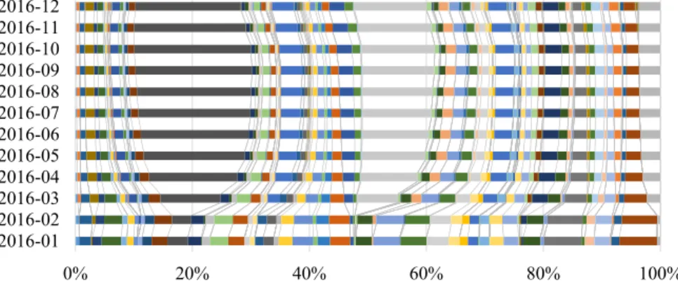
Page Figure 1.1 A case study of a pipeline with 5 queries. . . 6 Figure 4.1 Relative frequencies of different strata. The x-axis is the fraction of points
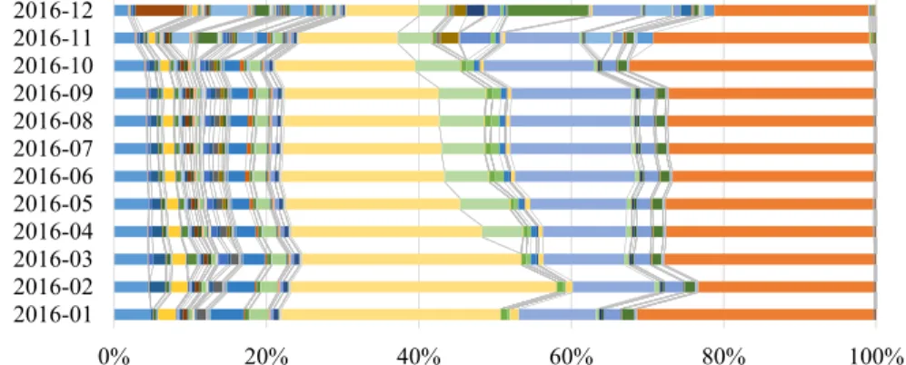
observed so far. At different points in time, the relative (cumulative) fre-quency of each stratum is shown. . . 46 Figure 4.2 Relative standard deviations of different strata, demonstrated by normalized
cumulative standard deviations observed by the end of each month. . . 47 Figure 4.3 The number of strata seen so far, and the number of records in data, as a
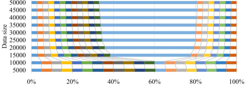
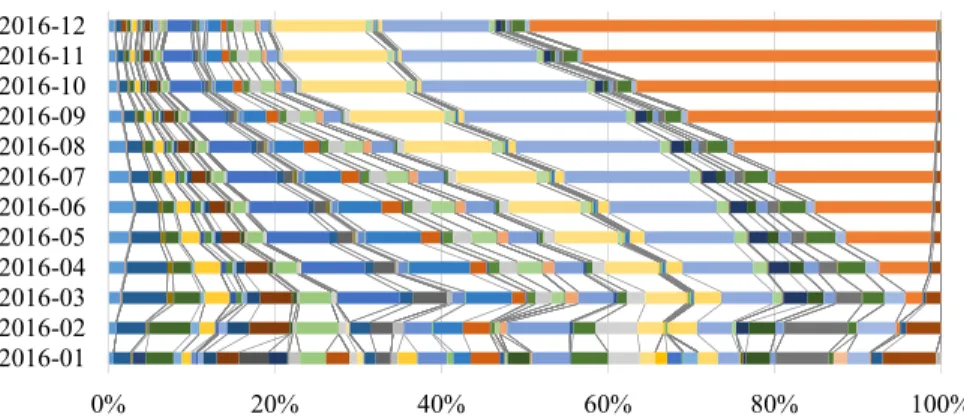
function of time. . . 47 Figure 4.4 Relative frequencies of different strata in the synthetic dataset change over
time. . . 48 Figure 4.5 Relative standard deviations of different strata in the synthetic dataset
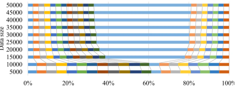
change over time. . . 48 Figure 4.6 Allocation of sample sizes among strata after 9 months, OpenAQ data . . . 49 Figure 4.7 Allocation due toVOILAchanges in allocation over time, OpenAQ data. . . 50
Figure 4.8 Allocation due to S-VOILA, with Single Element Processing, changes in
al-location over time, OpenAQ data. . . 50 Figure 4.9 Allocation due toS-VOILAwith minibatch processing, changes in allocation
over time, OpenAQ data. Batch size is one-day of data) . . . 51 Figure 4.10 Cosine distance between the allocations due toVOILA,S-VOILA with single
element processing, andS-VOILA with minibatch processing, OpenAQ data. 51
Figure 4.11 Variance ofVOILAcompares toNeymanandNeyman+with equal sample size:f
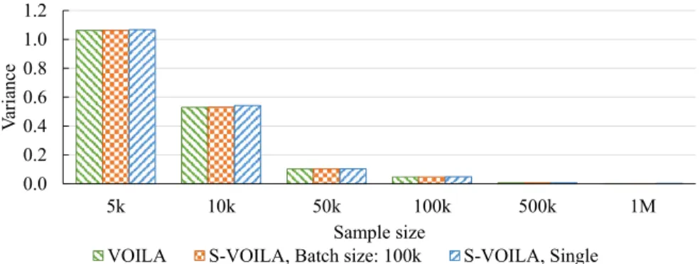
1M records, OpenAQ data. . . 52 Figure 4.12 Variance of streamingS-VOILA, with Single and Minibatch Processing,
com-pared with offlineVOILA. Sample size is set to 1M records, for each method,
Figure 4.13 Relative difference of the variance of S-VOILA, with Single and Minibatch
Processing, compared with the optimal variance due toVOILA, OpenAQ data. 53
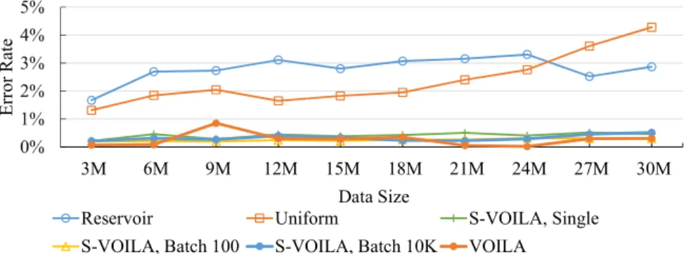
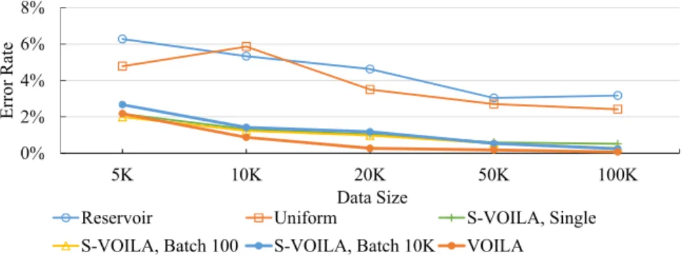
Figure 4.14 Impact of Sample Size on Variance, in September, OpenAQ data. . . 54 Figure 4.15 Impact of Batch Size on Variance, OpenAQ data. . . 54 Figure 4.16 Query Performance as data size varies, with sample size fixed at 100,000.
OpenAQ data. . . 55 Figure 4.17 Query Performance as sample size varies, with data size fixed at 21 million.
OpenAQ data. . . 56 Figure 4.18 Allocation due toVOILA across different strata changes over time, synthetic
dataset. . . 57 Figure 4.19 Allocation due to S-VOILA with Single Element processing changes over
time, synthetic dataset. . . 57 Figure 4.20 Allocation due to S-VOILA with Minibatch processing changes over time,
synthetic dataset. Batch size is 100. . . 58 Figure 4.21 The variance changes due to a sole change in synthetic data. . . 58 Figure 4.22 Query Performance on synthetic data as size of streaming data increases,
with sample size fixed at 1,000 and one stratum’s distribution changed at 10,000. . . 59
Figure 5.1 Maximum error forMASG query AQ1 andSASG query AQ3using a 1% sample. 83
Figure 5.2 Average errors, 1% CVOPTsample answers query AQ2 with weight settings. . 85
Figure 5.3 Average errors, 5% CVOPTsample answers query B1 with weight settings. . . 86
Figure 5.4 Sensitivity of maximum error to sample size. MASG query AQ2 answered by
samples with various sample rates. . . 87 Figure 5.5 Sensitivity of maximum error to sample size. SASG query B2 answered by
samples with various sample rates. . . 87 Figure 5.6 Maximum error of SASG queries with different predicates on OpenAQ,
an-swered by one materialized sample, showing the reusability of the sample. . 88 Figure 5.7 Maximum error ofSASGqueries with different predicates onBikes, answered
Figure 5.8 Maximum error ofCUBE group-by queries. . . 91
Figure 5.9 Comparison accuracy fromCVOPTandCVOPT-INFforSASGqueries AQ3and
B2. . . 92 Figure 6.1 Pipeline DAG forOpenAQuse case has one input table and 5 queries. . . 95
Figure 6.3 Join and Divide patterns, where different single-chained paths intersect. . . 97 Figure 6.4 The DAG forPrivEntdata pipeline. The execution order is from left to right.113
Figure 6.5 The distribution of the error of different approximate results on 5% sampled
PrivEntpipeline. The median error is less than 10% and the third quantile
of most of the aggregates are less than 20%. . . 114 Figure 6.6 The median error of the approximate results of different aggregates inPrivEnt
pipeline, at various sample rates. . . 114 Figure 6.7 The median error of the approximate results of Query3and Query5,OpenAQ
pipeline, at various sample rates. . . 115 Figure 6.8 Percentage of missing results in Query3,OpenAQpipeline and the final table
of thePrivEntpipeline, at various sample rates, comparing to the full results.116
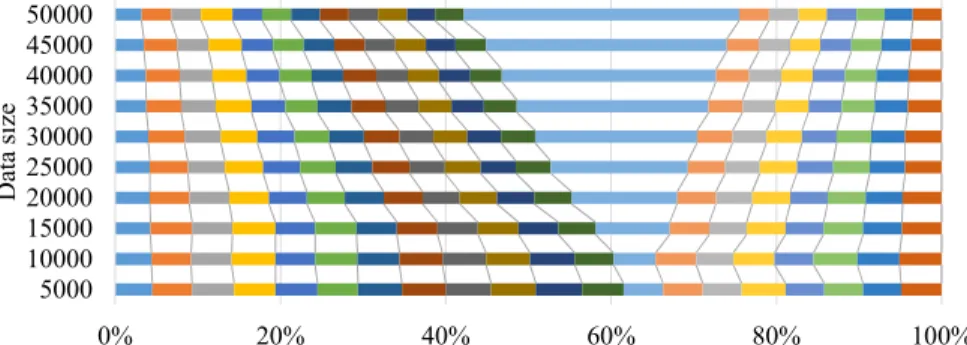
Figure 6.9 The exact and estimated results, with the 95% CI boundaries, of the esti-mation in Query3. Limited to top 50 results for the display purpose. . . 116 Figure 6.10 The exact and estimated results, with 95% CI boundaries, of thePrivEnt
pipeline. We hid the lables of the data. Limited to top 10.000 results for the display purpose. . . 117 Figure 6.11 CI coverage in Query 3, OpenAQ pipeline – percentage of true results fall
within the CIs boundaries. The coverages of computed CIs, at various quan-tile valuezl, are close to the expectation numbers. . . 118
ACKNOWLEDGMENTS
I would like to take this opportunity to express my thanks to those who helped me with various aspects of conducting research and the writing of this thesis. First and foremost, Dr. Srikanta Tirthapura for his guidance, patience, and support throughout this research and the writing of this thesis. His insights and words of encouragement have often inspired me and renewed my hopes for completing my graduate education. I would like to thank my colleagues and collaborators: Bojian Xu, Danny Ming-Hung Shih, Divesh Srivastava, Gabriela Jacques da Silva, Italo Lima, and Michael Levin for their enormous supports. It has been my privilege to work with each and every one of them. I would also like to express my thanks to my committee members for their efforts and contributions to this work: Dr. Suraj Kothari, Dr. Goce Trajcevski, Dr. Lizhi Wang and Dr. Mai Zheng. I would additionally like to thank Dr. Tien Nguyen for his guidance throughout the initial stages of my graduate career.
ABSTRACT
Data analysis consumes a large volume of data on a routine basis. With the fast increase in both the volume of the data and the complexity of the analytic tasks, data processing becomes more complicated and expensive. The cost efficiency is a key factor in the design and deployment of data warehouse systems. Approximate query processing is a well-known approach to handle massive data among different methods to make big data processing more efficient, in which a small sample is used to answer the query. For many applications, a small error is justifiable for the saving of resources consumed to answer the query, as well as reducing the latency.
We focus on the approximate query processing using random sampling in a data warehouse system, including algorithms to draw samples, methods to maintain sample quality, and effective usages of the sample for approximately answering different classes of queries. First, we study different methods of sampling, focusing on stratified sampling that is optimized for population aggregate query. Next as the query involves, we propose sampling algorithms for group-by aggregate queries. Finally, we introduce the sampling over the pipeline model of queries processing, where multiple queries and tables are involved in order to accomplish complicated tasks. Modern big data analyses routinely involve complex pipelines in which multiple tasks are choreographed to execute queries over their inputs and write the results into their outputs (which, in turn, may be used as inputs for other tasks) in a synchronized dance of gradual data refinement until the final insight is calculated. In a pipeline, approximate results are fed into downstream queries, unlike in a single query. Thus, we see both aggregate computations from sampled input and approximate input.
We propose a sampling-based approximate pipeline processing algorithm that uses unbiased estimation and calculates the confidence interval for produced approximate results. The key insight of the algorithm calls for enriching the output of queries with additional information. This enables the algorithm to piggyback on the modular structure of the pipeline without having to perform any
global rewrites,i.e.,no extra query or table is added into the pipeline. Compared to the bootstrap method, the approach described in this paper provides the confidence interval while computing aggregation estimates only once and avoids the need for maintaining intermediary aggregation distributions.
Our empirical study on public and private datasets shows that our sampling algorithm can have significantly (1.4 to 50.0 times) smaller variance, compared to the Neyman algorithm, for optimal sample for population aggregate queries. Our experimental results for group-by queries show that our sample algorithm outperforms the current state-of-the-art on sample quality and estimation accuracy. The optimal sample yields relative errors that are 5×smaller than competing
approaches, under the same budget. The experiments for approximate pipeline processing show the high accuracy of the computed estimation, with an average error as low as 2%, using only a 1% sample. It also shows the usefulness of the confidence interval. At the confidence level of 95%, the computed CI is as tight as±8%, while the actual values fall within the CI boundary from 70.49%
CHAPTER 1. OVERVIEW
1.1 Introduction
A data warehouse system handles a large volume of data on a routine basis to process various data consumption applications. Over time, we see the humongous increases in both the scale of the data and the complexity of the analytic tasks. The data processing becomes more complicated and thus more expensive. The cost efficiency is a key factor in the design and deployment of data warehouse systems.
Approximate query processing is a well-known approach to handle massive data Acharya et al. (1999a);Agarwal et al.(2014);Babcock et al.(2003);Cao and Fan(2017);Chakrabarti et al.(2001); Chaudhuri et al.(2001a), among different methods to make big data processing more efficient, such as indexingDing et al.(2016);Subotic et al.(2018);Wang et al.(2015a), cachingAdali et al.(1996); Zhao et al.(2014), sketchingAnderson et al.(2017);Basat et al.(2018), view materializationHanson (1987);Uchiyama et al.(1999),etc.. Random sampling has been widely used in approximate query processing on large databases Chaudhuri et al. (2017); Chen and Yi (2017); Thompson (2012); Wu et al. (2016); Kandula et al. (2016a); Till´e (2006); Nguyen et al. (2016). Random sampling has the potential to significantly reduce resource usages and response times, at the cost of a small approximation error. In fact, for many applications, the exact answer is unnecessary. Thus a small error is justifiable for the saving of resources consumed to answer the query, as well as reducing the latency. For example, given a query that powers a visualization dashboard where its result is displayed as a figure. The errors in the query answer lead to incorrections in the figure. Most of the time, the small differences in visualization are tolerable. Especially, when the errors are small enough, the difference between approximate and exact figures are virtually unnoticeable. While sampling gives us the flexibility of answering various queries, it does not require so much extra storage space. This feature makes sampling stands out from other approaches to answering big
query efficiently such as caching, pre-computation, or view materialization. While those methods can give the exact answers for the supported set of queries, the size of the additional space needed is proportional to the number of supported queries. When the business needs are involved, sampling becomes a good choice over other approaches, in terms of the ability to work with complex data processing model.
In this work, we focus on the approximate query processing using random sampling in a data warehouse system, including algorithms to draw samples, methods to maintain sample quality, and effective usages of the sample for approximately answering different classes of queries. We study different methods of sampling, focusing on stratified sampling that is optimized for population aggregate query and group-by query. Last but not least, we introduce the sampling over the
pipeline model of queries processing, where multiple queries and tables are involved in order to accomplish complicated tasks.
The pipeline model allows the user to break down their analysis into multiple steps, in which each step is relatively smaller. The pipeline is not only helpful in making the analytic task more readable and easier to debug and maintain, but also useful in the modularity of the analysis. With the pipeline model, data flow becomes logical and intermediate results can be reused. The pipeline model has been widely studied and used Jacques-Silva and Zhang (2018); Bowers et al.; Pfleiger et al.;Huang et al..
We will focus on the computation of confidence interval for the estimations when we apply a sample algorithm on a pipeline. Since the results from the sample are approximated, one of the main concerns of sampling’s usefulness is how good or bad the approximations are, i.e., how far way the estimates are from the ground-truth answers. The confidence interval is a good measure-ment that can be used as enforcemeasure-ment for each estimated result. In traditional sampling models, confidence interval has been widely studied Haas (1997); Cohen (1994); Johns (1988); Schenker (1985); Nedelman et al. (1995). Numerically, it can be present along with the estimate, e.g., the estimatex= 100±5 says the estimated value ofx is 100 and, with high probability, the unknown
As the pipeline model is complex, computing the confidence for the estimation is challenging. The aggregates that are directly on the sampled table have the information about the randomness, but downstream aggregates, which query on top of the approximate tables, do not have this infor-mation. The needed information has been propagated along with the main results in the pipeline. Secondly, there are many different computation operators in a pipeline, in which provide confidence interval is not always trivial. Even for those operators that confidence interval is well formulated, each of them requests different intermediate information to have the confidence interval computed. Simply combining all the needed information is infeasible. The number of extra works will blow up the complexity of the pipeline, which is already complicated.
By addressing the challenging problem of computing confidence interval for sampled estimations in the pipeline computational model, we are expected to significantly improve the usefulness of approximate query processing, especially for complex pipelines. The confidence interval not only provides the measurement of estimate’s accuracy but also leads to the tremendous potential of applications, related to using sampling, such as optimizing the sample rate, dynamic sampling,
etc..
1.2 Approximate Query Processing
Approximate query processing is essential for handling massive data. Different methods of approximations provide interactive response time when exploring massive datasets, and are also needed to handle high-speed data streams. Some methods are lossless, while others are lossy compaction of the data. But they share the same high-level approach of using synopsis rather than the entire dataset. The synopsis could be composed in different ways, include, but not limited to, random samples Babcock et al.(2003); Ganti et al. (2000);Haas (1997); Brown and Haas (2006), histograms Chaudhuri et al. (1998); Muralikrishna and Dewitt(1988); Ioannidis(1993); Ioannidis and Poosala(1995), waveletsCormode et al.(2011);Gilbert et al.(2001);Vitter and Wang(1999), sketches Tirthapura et al. (2006); Xu et al. (2008); Cormode et al. (2007); Indyk et al. (2000), materialized views Olken and Rotem(1992);Hanson(1987); Uchiyama et al.(1999),etc.. Each of
such synopsis captures vital properties of the original massive data while typically occupying much less space. For example, given the original data consists of large time serial numbers, we can have a materialized view that pre-computes the number of observations, n; the sum of all the values, X
x; the sum of the squares of the values,Xx2. This view helps not only with the pre-computed
aggregates but also aggregates referred on top of it, such as with the ratio of the sum and the count is the average, Px
n , and the variance is a ratio of the sum of squares to the count, less the square
of the average, P x2 n − Px n 2 .
In the above example, the aggregates are lossless, however, we may need to know more about the data than merely its variance. The other estimations may not have such properties, or even can’t be composed because the view with three-value summary does not suffice. To answer more various types of queries, an appropriate type of synopses are needed. In general, any type of approximate query processing, no matter how complex they are to compute, will have weak points. Indeed, for many of these questions, no synopsis can provide the exact answer. For example, the row-select query, the query answers collectively describe the data in full, and so any synopsis would effectively have to store the entire dataset. Other cases are when the result of the query is error-sensitivity,
i.e.,the query to create bills, fill out tax information, etc..
Nonetheless, a wide range of classes of the query, where the small error can be tolerated, can be well supported by approximate query processing. In these cases, the requirements are much relaxed. The key objective is not obtaining the exact answer to a query, but rather receiving an accurate estimate of the answer. e.g., receiving an answer that is within 1% of the true result is adequate for most of the cases. It might suffice to know that the true answer is approximated
x≈1×10⁶, without knowing that the exact answer isx= 1,010,483.6367. Thus we can tolerate
approximation. Such synopses that provide approximate answers are practically useful in analytic applications that process large datasets.
As approximate query processing is widely applied in practice, the research community has also been studying it thoroughly in multiple aspects such as accuracy, space and time efficiency, optimality, error bounds on query answers, incremental maintenance,etc..
1.3 Query-based Sampling Algorithms
We design sampling algorithms to serve different classes of queries, starting from the simple population aggregate query, that produces a single aggregation. Next, we design sampling algo-rithms for the group-by query, in which the answer is a collective aggregate result. Lastly, we target the complex query pipeline where it involves multiple queries.
For the simple query of population aggregate, general unbiased sample,e.g.,uniform sample, is straightforward to implement and can be widely used. However, the sample may not well represent the original data. For example, given a simple dataset of 1000 elements, that contains 990T rues and
10 F alses, a uniform sample high likely contains all theT rueelements. Otherwise, to haveF alse
values represented, the uniform sample will be relatively large, which is again the purpose of using the sample. Stratified random sampling is a fundamental biased sampling technique that provides accurate estimates for aggregate queries using a small size sample, and has been used widely for approximate query processing. A key question in stratified sampling is how to partition a target sample size among different strata. While Neyman allocationNeyman (1934) provides a solution that minimizes the variance of an estimate using this sample, it works under the assumption that each stratum is abundant,i.e.,has a large number of data points to choose from. This assumption may not hold in general: one or more strata may be bounded, and may not contain a large number of data points, even though the total data size may be large.
We present VOILA, an offline method for allocating sample sizes to strata in a variance-optimal
manner, even when one or more strata may be bounded. Our results from experiments on real and synthetic data show thatVOILAcan have significantly (1.4 to 50.0 times) smaller variance than
Neyman allocation.
Next step, we target a more complex query class with a group-by clause. This is a widely used type of query where the query firstly groups data according to one or more attributes, and then aggregate within each group after filtering through a predicate. The challenge with group-by queries is that a sampling method cannot focus on optimizing the quality of a single answer (e.g.
table1 table3 table4 table5 Query1 Query2 Query3 table6 Query4
Logging system
Dashboard system Pipeline table2Figure 1.1: A case study of a pipeline with 5 queries.
the mean of selected data), but must simultaneously optimize the quality of a set of answers (one per group).
We presentCVOPT, a query- and data-driven sampling framework for a set of queries that return
multiple answers, e.g., group-by queries. To evaluate the quality of a sample, CVOPT defines a
metric based on the norm (e.g. `2 or`∞) of the coefficients of variation (CVs) of different answers
and constructs a stratified sample that provably optimizes the metric. CVOPT can handle group-by
queries on data where groups have vastly different statistical characteristics, such as frequencies, means, or variances. CVOPT jointly optimizes for multiple aggregations and multiple group-by
clauses and provides a way to prioritize specific groups or aggregates. It can be tuned to cases when partial information about a query workload is known, such as a data warehouse where queries are scheduled to run periodically.
Our experimental results show that CVOPT outperforms the current state-of-the-art on sample
quality and estimation accuracy for group-by queries. On a set of queries on two real-world data sets, CVOPT yields relative errors that are 5×smaller than competing approaches, under the same
budget.
1.4 Pipeline of Queries in the Data Warehouse
Not only the volume of the data but also the complexity of the analysis tasks is increasing over time. Gaining the non-trivial insights requites complicated explorations and mutations of the
data. Eventually, a single query is not sufficient to efficiently handle complex tasks. To address the problem, the model of the pipeline of queries is introducedJacques-Silva and Zhang (2018).
A pipeline of queries, or a pipeline – in short, is a collection of queries and tables, placed in a topological order of execution. A pipeline is a directed acyclic graph (DAG), where the tables are represented by nodes and the queries are denoted by edges. The results of a query are materialized as a table, that may serve other queries down the stream. Figure1.1shows an example of a pipeline that consumes data from a logging system to power a visualization dashboard. The pipeline contains 4 queries and 6 tables. Instead of a single complicated query, that joins all the source tables to do such massive computation at one, the pipeline breaks the complex task into sub-tasks. It organizes the computation as a DAG of sub-tasks and intermediate results. Each sub-task can be done by a much smaller query. Due to the great benefits that the model provides, it has been practically adopted in industrial, large-scale data warehouse systems Jacques-Silva and Zhang(2018);Bowers et al.;Pfleiger et al.;Huang et al..
The pipeline model brings multiple benefits, especially in a large-scale setting:
• Modularity: The complex task is broken down into multiple components, each is well defined and is designed to achieve a single or few intermediate results. Data engineers have better control over their pipeline. Multiple small, easy to understand components are easier to debug, maintain, and evolve the analysis than a huge, super-complicated query.
• Readability: Complex task makes the query hard to read to humans, especially with SQL language, since it is not designed to carry the logic as a programming language. Thus, having self-contain components reduces complexity. Each query in the pipeline can be as simple as doing a projection or an aggregation, make them easily understandable.
• Reusability: Even with highly optimized query engines, the complex tasks may lead to redundancy in query computation. In the pipeline model, intermediate results are materi-alized. Thus, they can be reused instead of duplication in the computation. Furthermore,
intermediate results can also be shared among pipelines. In practical deploy, data warehouse systems have tables that served multiple pipelines.
• Scalability: The pipeline model allows the system to be scaled in both the magnitude of the data and the number of tasks can be processed. The supporting infrastructure is a combination of multiple workers. Instead of having one worker do a complex task, a pipeline can be processed by multiple workers in parallel.
1.4.1 Approximate Query Processing with Pipeline
As large-scale data analysis is expensive, while many tasks do not require the exact answer, approximate query processing is a good approach to reduce resource consumption. Random sam-pling has been widely used in approximate query processing, especially for data warehouse set-tingChaudhuri et al.(2017);Chen and Yi(2017);Thompson(2012);Cochran(1977);Lohr(2009); Till´e (2006). Traditionally, with single query processing, the approximate answer is derived from the sampled table where the randomness can directly be handled. In this work, we present a model of random sampling for the pipeline of queries. As the pipeline is a complex data processing model where not only one query but a collection of queries are involved, the approximate answer of one query becomes the input for another query. Thus the uncertainty is carried out and controlling the randomness becomes much more complicated.
In the pipeline model, when a table is sampled, the part following it contains approximate results. Also, there may be multiple input tables involved. Different choices of samples to be sampled lead to the different schema of applying sampling for a pipeline. We observe that the processing of a query over a sampled table is different than of the query over an approximate table. The sampled table contains a subset of the data, in which each record is an actual observation from the original data. The randomness in estimating from those tables is from whether or not each record is selected into the sample. On the other hand, in the approximate table, the records are estimated. Thus, not only may a subset of the original results are seen, but the observed data itself
contains uncertainty. Therefore, applying sampling over the pipeline query model is challenging and non-trivial.
1.4.2 Confidence Interval
Sampling has been shown to be an efficient approach to handle massive data in the warehouse. By querying to the sample table, which has a subset of the data, we consume fewer resources and the user gets results faster. The trade-off is that answers are not exactly accurate, rather they are approximate answers. While exact answers are not necessary for most of the business needs, users still demand to know how accurate the approximate answers are. Confidence Interval (CI) can enrich the estimation. The CI of an estimationx is a range in such with high probability the
true value belongs to:
x∈[¯x−δ; ¯x+δ]
In which ¯xis the unbiased estimation ofx, andδ is the CI of this estimation. The estimation is also
written in form of x≈x¯±δ. For example, given a 90% CI of an approximate count query answer
is 100±5, we can expect that, with 95% certainty, the true count is between 95 and 105. The CIδ
not only tells the user how accuracy each aggregate but also be used in different applications, such as to visualize the error bar and to guide the user on deciding the sample rate,etc..
While building suppuration, both theoretically and systematically, to sampling for a complex pipeline of queries, integrating CI computation as a part of the sampling model is essential. In opposite to computing the CI for a single query, providing CI for a pipeline of queries is non-trivial, due to the complexity of the pipeline as well as the model we have to execute the pipelines. For example, on the pipeline described in Figure 1.1, the computation of a SUMaggregate in Query 1,
that takes sampled table1 as input, is different than a SUM aggregate of Query 4, that queries to
an approximate table5. A pipeline is a complicated DAG of multiple queries, each query may be
complicated and has nested queries. Each node in the DAG is processed at a time. Intermediate results are materialized as a table, thus at the final step, where the actual output is computed, tracing back up to the input tables, where we apply sampling is impractical. The intermediate
results are needed to be carried on along the pipeline. Along with the approximate query processing, using sampling, over the pipeline model, we introduce the integrated computation of the CI.
CHAPTER 2. PROBLEM STATEMENT
We first define the problem we aim to solve in this work, followed by the motivation for the research as well as the challenges of solving it.
Problem statement: Design the computational models for approximate query processing, includ-ing drawinclud-ing the query-driven optimal random samples and efficiently usinclud-ing the random sample in a data warehouse setting.
Approximate query processing is a powerful approach to handling large-scale data sets. Sampling is commonly used in approximate query processing as the sample is smaller, thus it is cheaper to query upon but can well represent the original data. Where the small error is tolerable, approximate query processing is very useful in reducing resource consummations as well as reduce latency.
We proposed sample algorithms to draw the sample that best represents the data. Although a uniform random sample is simple and widely used, it selects records into the sample uniformly at random. The sample does not well represent the original data as underpopulated groups may be missing or underrepresented in the sample. With the same sample space, given information about the original dataset, we can have a better representative by a biased sample that captures the frequency skewness of the data, especially in representing infrequent portions of the data. Moreover, given both the data statistics and the information about the query workload, i.e., the classes of the query, that the data serves, we aim to draw the sample that not only well represents the data but also be optimal to serve the queries.
Although random sampling has been studied along with the history of data processing, drawing and maintainingoptimal samples are challenging:
• The definition of anoptimal sample is unclear, thus creating a good random sample is nontriv-ial. A universal optimal sample is unachievable as the sample is only the synopsis constructed
from a subset of the data, no sample can serve all queries, especially with a selective query that the result depends on a single record. Thus, we first narrow down the target to be the sample is drawn to serve aggregate queries.
• The query can have a group-by clause, in which data is divided into groups. Since data distribution of each group varies significantly, we classify the aggregate queries into 2 subsets: population aggregate and group-by aggregate. In other words, we aim to serve 2 different classes of SQL queries, with and withoutGROUP BY clause. This strategy helps us address the challenge of defining the measurement of how good a sample is.
• The reusability of the sample is a strong requirement. Creating a sample for each query is expensive and against the purpose of reducing resource consumption. On the other hand, each query is unique due to the power of the query language. The SQL query is very flexible, a query can be a combination of multiple aggregates, with or without predicates, groups by, join, etc.. And a query can have multiple nested subqueries. We aim to create a sample that can be reused for multiple queries.
Furthermore, we apply the sampling in approximate query processing in the pipeline - a complex data warehouse settings. The pipeline model breaks a complex data analysis task into multiple steps, in the form of a DAG of queries and intermediate results, as shown in Figure1.1. The sampled table not only serves a single query but multiple queries. Moreover, the estimated results are fed into downstream queries. When the uncertainty is amplified after each step, the computation of unbiased estimation in downstream steps is nontrivial. Moreover, providing the confidence interval for the estimation is challenging, due to the lack of direct information of the randomness. Each estimate has its own unique computation, which depends on not only the function but its position in the complex DAG. We aim to provide a systematic computation model that derives both the unbiased estimate and its confidence interval for the approximate pipeline.
We introduce the sampling model that not only delivers the approximate results but also the
and δ are the unbiased estimation and the CI of the estimation x. For example, while the true
value of an sum aggregate is SU M = 10242 while its estimation could be SU M ≈ 10000±500.
As the answers are approximated, naturally, providing a good measurement of the accuracy of the estimate becomes essential. The Confidence Interval is a good method to do such measurements. The confidence interval provides a measure of accurateness of the estimate as they are needed in any approximate answer. Moreover, the confidence interval also provides a means to strengthen the sampling over a pipeline, in which it can be incorporated in the sample selection procedure and sample rate decision.
The great usefulness of the confidence interval comes with several challenges to compute it. • Computing confidence interval is non-trivial. The computation is by operators. While some
operators, such as Sumand Count, have the confidence interval well defined, others, such as Max, Percentile,etc., are not clear.
• The pipeline of queries is complex. Not as a traditional sampling model where the sample is drawn from a single table, in the pipeline model there are multiple tables involved. As multiple sources of randomness are present, the computation of confidence interval becomes more complicated.
• The non-directed computation in the pipeline. In a simple sampling instance, the sample is drawn from a single table, and estimations are upon such a single sample. On the other hand, a pipeline is a DAG of queries. For maximizing the effect of resource-saving, the samples tend to be in the early stages of the pipeline. Meanwhile, the confidence intervals are needed at the final step of the pipeline. Following the flow of computation, queries are on top of the estimated results. Such indirect computation is challenging.
• Exponential of the computation space. As the covariance of different attributes is needed in the computation, providing all the covariance of all combinations is infeasible.
2.1 Approach
In this work, we firstly study the approximate query processing, using the sample table, on a large-scale. This study builds up the basic statistic and optimization backgrounds for using sampling. Since sampling has been thoroughly studied in the research community as well as widely used in industrial systems and applications, we start by reviewing the literature of using sampling. Next, we focus on studying stratified sampling, an interesting sampling method that advances the sample power to serve approximate query processing better with limited given resources. We propose sampling algorithms that fit the specific purpose of query processing, particularly, to serve the aggregate queries, with and without group-by.
Secondly, we introduce the sampling for the model of the query pipeline. We start with the based model of the pipeline, computation method, and a case study pipeline. We then focus on computation models for supporting sampling on the query pipeline. The main challenge we aim to address is to provide a confidence interval for each estimated result computed in the pipeline. We propose a model to compute the confidence interval for a set of commonly used aggregate functions. Not only address the problem of computing confidence interval, but we also show the usefulness of the confidence interval in approximate query processing. The confidence interval is not only enriching the estimated results but also provides a means to optimize the sampling model. For example, one research question that we aim to address is using the confidence interval to allocate the sample space. Optimizing sample space by the characteristic of the dataNguyen et al.(2019); Cormode et al. (2011);Ding et al. (2016) has been well studied. With confidence interval, we can optimize sample size based on user-defined error bound as well.
2.2 Contributions
This research aims at contributing a novel model of drawing and using random sampling in approximate query processing.
1. We study the problem of approximate query processing in a massive data warehouse. By using different methods of sampling, including uniform and stratified sampling, we show to the potential of reducing resource consumption and shorten the query latency in processing large datasets.s
2. We proposed query-driven random sampling algorithms, that create and maintain the optimal samples based on statistics of the dataset and the knowledge of the query workload, in both streaming and static data management manner.
3. We introduce the approximate query processing for the query pipeline model. While the pipeline model allows a complicated task to be broken down into small, manageable sub-tasks, applying sampling on top of it further reduce the cost of processing complex task. 4. We design the method to compute both the unbiased estimation and the confidence interval
for each estimation in approximate pipeline processing. The method support projection, basic algebra operators, and common aggregate COUNT, SUM, and AVG. Join is partially supported under a certain assumption that guarantees the equivalent of sampling apply before and after joining.
CHAPTER 3. REVIEW OF LITERATURE
In this chapter, we study the background knowledge from previous works, including sampling techniques and approximate query processing, over static or streaming data. We present the state-of-art technologies and we also discuss what contribution we could make in this research field. We study the background knowledge in the computational model of the query pipeline.
3.1 Approximate Query Processing
Approximate query processing methods are necessary for dealing with massive data and has been extensively studied Chaudhuri et al. (2017); Babcock et al. (2003); Agarwal et al. (2014); Ganti et al. (2000); Peng et al. (2018); Flajolet (1985); Gilbert et al. (2001); Goldreich (1997); Brown and Haas(2006). They are good means of reducing interactive response times and resource consummations when exploring massive datasets. These common methods proceed by computing a lossy, compact synopsis of the data, and then executing the query of interest against the synopsis rather than the entire dataset.
Histograms have been well studiedGibbons et al.(1995);Ioannidis and Christodoulakis(1993); Gilbert et al. (2002) and have been incorporated into the query optimizers of virtually all com-mercial relational databases. It summarizes a dataset by grouping the data values into subsets, or “buckets”, and then, for each bucket, computing a small set of summary statistics that can be used to approximately reconstruct the data in the bucket.
Sketch summaries are particularly well suited to streaming data Tirthapura et al. (2006); Xu et al. (2008); Cormode et al. (2007); Indyk et al. (2000). Linear sketches, for example, view a numerical dataset as a vector or matrix and multiply the data by a fixed matrix. Such sketches are massively parallelizable. They can accommodate streams of transactions in which data is both
inserted and removed. Sketches have also been used successfully to estimate the answer to COUNT DISTINCT queries, a notoriously hard problem.
Histograms and sketch share a drawback of limited usage. These synopses are highly compact and particularly good for the set of designed queries, but they are lack of the generality to handle ad-hoc queries. Sampling is a relatively more expensive synopsis, that better captures the baseline data. Sampling has been the most widely used in approximate query processing on both staticChaudhuri et al. (2017); Chen and Yi (2017); Thompson (2012); Cochran (1977); Lohr (2009); Till´e (2006) and streaming dataNguyen et al.(2019);Hentschel et al.(2018);Haas(2016);Zhang et al.(2016); Ahmed et al.(2017). The reservoir samplingMcleod and Bellhouse(1983);Vitter(1983) method for maintaining a uniform random sample on a stream has been known for decades, and many variants have been considered, such as weight-based sampling Efraimidis and Spirakis (2006); Braverman et al. (2015), stream sampling under insertion and deletion of elements Gemulla et al. (2008), distinct sampling Gibbons and Tirthapura(2001), sampling from a sliding windowBabcock et al. (2002b);Gemulla and Lehner(2008);Braverman et al.(2009), and time-decayed samplingCormode et al. (2009b,a). We discuss random sampling in the next section.
A majority of prior work on using stratified sampling in approximate query processingAcharya et al.(1999a,2000);Chaudhuri et al.(2007);Joshi and Jermaine(2008);Agarwal et al. (2013) has assumed static data. With the emergence of data stream processing systemsBabcock et al.(2002a) and data stream warehousing systems Johnson and Shkapenyuk (2015), it is important to devise methods for streaming stratified sampling with quality guarantees.
3.2 Random Sampling
Over the decades, many researchers have been studying different sampling techniques based on statistics to improve the accuracy of the collected sample Cochran (1977); Lohr (2009); Mcleod and Bellhouse (1983);Thompson(2012); Till´e(2006). In the following paragraphs, we will briefly introduce the background knowledge of some sampling techniques, including uniform sampling and stratified sampling.
Uniform random sampling also known assimple random sampling, is a method to draw a random sample in which the element is selected uniformly at random Cormode et al. (2011);Lohr (2009); Till´e(2006). In other words, each individual in the population is chosen with the same probability. For example, if we want to sample m elements from a population of n elements (m < n), each
element in this population has equal probability of m
n to be chosen into the sample set.
Reservoir sampling Vitter (1985,1983);Efraimidis and Spirakis(2006) is an extended random sampling technique for streaming data, that guarantees equal probability of selecting each element in a population without prior knowledge of population size. Reservoir sampling is commonly known for its usefulness in data streaming where total length is unknown.
Stratified sampling is a biased sampling, where the population is partitioned into subgroups called “strata”. From within each stratum, uniform random sampling is used to select a per-stratum sample. All per-stratum samples are combined to derive the “stratified random sample”. Stratified random sample in the online setting Thompson (2012) can be viewed as a type of weight-based reservoir sampling where the weight of each stream element is changing dynamically, based on the statistics of the stratum the element belongs to. Since the weight of each stream element changes dynamically, even after it has been observed, prior work on weighted reservoir samplingEfraimidis and Spirakis(2006) does not apply here, since it assumes that the weight of an element is known at the time of observation and does not change henceforth. Meng Meng(2013) considered streaming stratified sampling using population-based allocation. Al-Kateb et al. Al-Kateb and Lee (2010, 2014) considered streaming stratified sampling using power allocation, based on their prior work on the adaptive reservoir sampling Al-Kateb et al. (2007). Lang et al. Lang et al. (2016) consider machine learning methods for determining the per-item probability of inclusion in a sample. This work is meant for static data and can be viewed as a version of weighted random sampling where the weights are learned using a query workload.
Specified samples, that is optimized for the given query workload or query pattern, is well studied. Ganti et al. Ganti et al. (2000) addresses low selectivity queries using workload-based sampling, such that a group with a low selectivity is sampled as long as the workload includes
queries involving that group. Different techniques have been used in combination with samplings, such as indexing Ding et al. (2016); Wang et al. (2015b); Chaudhuri et al. (2001b), or aggregate precomputationPeng et al. (2018).
Chaudhuri et al. Chaudhuri et al. (2007) formulate approximate query processing as an opti-mization problem. Their goal is to minimize the `2 norm of the relative errors of all queries in
a given workload. Their approach to group-by queries is to treat every group derived from every group-by query in the workload as a separate query. In doing so, their technique does not han-dle overlap between samples suited to different groups. In contrast, our framework considers the overlaps and interconnections between different group-by queries in its optimization.
Kandula et al.Kandula et al.(2016b) consider queries that require multiple passes through the data and use random sampling in the first pass to speed up subsequent query processing. This work can be viewed as query-time sampling while ours considers sampling before the full query is seen. Further,Kandula et al.(2016b) does not provide error guarantees for group-by queries, as we consider here. A recent workNguyen et al. (2019) has considered stratified sampling on streaming and stored data, addressing the case of full-table queries using an optimization framework. This work does not apply to group-by queries.
R¨osch and LehnerR¨osch and Lehner(2009) propose non-uniform sampling to support group-by queries, where different groups can have vastly different variances. This proposed algorithm is a heuristic without a guarantee on the error, and in fact, does not have a well-defined optimization target. In our work, we will study a sample algorithm that has provable guarantees holding even in case of multiple aggregations and/or multiple group-bys.
“Congressional sampling” Acharya et al. (2000) targets sampling for a collection of group-by queries, especially those that consider a “cube by” query on a set of group-by attributes. Congres-sional sampling is based on a hybrid of frequency-based allocation (the “house”) and fixed allocation (the “senate”). However, congressional sampling ignores the coefficients of variation (and hence also the variances) of different strata in deciding allocations, it only uses the frequency. That results in a non-optimal allocation.
A recent work “Sample+Seek”Ding et al.(2016) uses a combination of measure-biased sampling and an index to help with low-selectivity predicates. Measure-biased sampling favors rows with larger values along with the aggregation attribute. This does not consider the variability within a group in the sampling step – a group with many rows, each with the same large aggregation value, is still assigned a large number of samples. Thus, it does not favor groups with larger CVs. Note that those groups with larger variations in the aggregation attribute. Further, “Sample+Seek” does not provide a sampling strategy that is based on an optimization framework.
3.3 Approximate Pipeline Processing in Data Warehouse
Approximate query processing is a well-known approach to conduct analysis over massive data Acharya et al. (1999a); Agarwal et al. (2014); Babcock et al. (2003); Cao and Fan (2017); Chakrabarti et al. (2001); Chaudhuri et al. (2001a). Among different synopses, such as indexing, caching, and sketching, random sampling has been widely used to approximate results of queries on large databases Chaudhuri et al. (2017); Chen and Yi(2017); Wu et al.(2016); Kandula et al. (2016a); Nguyen et al.(2016).
The data pipeline model is commonly used on the analysis of large datasets as it enables us to break down complex tasks into a flow of manageable sub-tasks. Applying AQP on top of the data pipeline model potentially reduces the resources needed for processing massive datasets while still resulting in good approximations. This is the case, especially when considering that samples of massive datasets are still pretty large, resulting in a good representation of the original dataset. To the best of our knowledge, this work is the first to describe the application of sampling on a data pipeline and detailing how we can do the computation of confidence intervals on such scenarios.
For a single-step AQP, the statistical inequalities and the central limit theorem has been used to compute the CI of the approximate result Chaudhuri et al. (2007); Hu et al. (2009); Wu et al. (2010). Pansare et al. Jermaine et al. (2007) developed a Bayesian framework to infer the CI of the approximate answers. However, this approach is limited to simple group-by aggregate queries. Other works have focused on specific types of queries. Charikar et al. Charikar et al. (2000)
studied distinct value estimation from a sample; Jermaine et al. Jermaine et al. (2005) proposed an algorithm to quantify aggregate queries with subset testing. These works neither provide a systematic way of computing the confidence interval nor are able to handle the query pipeline scenario, where the randomness information, for the most part, is not directly accessible.
An alternative approach to compute the confidence interval for approximations is bootstrap, a method adopted from statistics studies Bickel et al. (1981); Efron and Tibshirani (1994); Kleiner et al.(2013). In the database community, recent worksAgarwal et al.(2014);Zeng et al.(2014);Pol and Jermaine (2005) have used bootstrap to quantify the quality of approximate query answers. Although bootstrap can support a wider range of aggregation queries, it is known to be costly, due to its resample procedure and multiple tries in order to have reliable results. Pol et al. Pol and Jermaine (2005) focus on efficiently generating bootstrap resamples in a relational database setting, while Laptev et al. Laptev et al. (2012) target MapReduce platforms and study how to overlap computation across different bootstrap resamples. Nonetheless, the computational cost of bootstrap is far more expensive than those of the original sampled query, which is directly against the purpose of approximate query processing. Especially in complex query model, such complexity is amplified as the pipeline contains multiple queries.
CHAPTER 4. OPTIMIZED SAMPLE SPACE ALLOCATION FOR POPULATION ESTIMATE
In this chapter, we discuss stratified random sampling (SRS) and optimizing the sample space for SRS to serve population estimates. First, we present an offline algorithm for variance-optimal SRS for data that may have bounded strata. Our algorithm VOILA (VarianceOptImaL Allocation)
computes an allocation that has provably optimal variance among all possible allocations of sample sizes to different strata. While prior work assumes that there are no strata with small volumes of data, which is often violated in real data sets, our analysis makes no such assumptions. VOILA is
a generalization of Neyman allocation and reduces to Neyman allocation in the case when every stratum is abundant.
We present a lower bound showing that any streaming algorithm for SRS that uses a memory of
M records must have, in the worst case, a variance that is a factor of Ω(r) away from the variance
of the optimal offline algorithm for SRS that uses a memory of M records. This lower bound is
tight since there exist streaming algorithms for SRS whose variance matches this bound in the worst case.
We present S-VOILA, a streaming algorithm for SRS that is locally optimal with respect to
variance – upon receiving new elements, it (re-)allocates sample sizes among strata so as to minimize the variance among all possible re-allocations. S-VOILA can be viewed as the online, or dynamic
counterpart of the optimization that led toVOILA, which is based on optimizing the variance using
a static view of data. S-VOILA can also deal with the case when a minibatch of multiple data
items is seen at a time, rather than only a single item at a time – re-allocations made by S-VOILA
are locally optimal with respect to the entire minibatch and are of higher quality for larger size minibatches than when a single element is seen at a time. In our experimental study, we found that the variance of S-VOILA is typically close to that of the offline algorithm VOILA, and the variance
of S-VOILA improves as the size of the minibatch increases. Since it can deal with minibatches of
varying sizes, it is well-suited to real-world streams that may have bursty arrivals.
The algorithms for offline SRS (VOILA) and streaming SRS (S-VOILA) are both based on a
technique for reducing the size of an existing stratified random sample down to the desired target size such that the increase in the variance of the estimator based on the final sample is optimized. This technique for sample size reduction may be of independent interest in other tasks such as sub-sampling from a given stratified random sample.
We present a detailed experimental evaluation using real and synthetic data, considering both the quality of the sample and the accuracy of query answers. Our experiments show that (a)VOILA
can have a significantly smaller variance than Neyman allocation, and (b) S-VOILA closely tracks
the allocation as well as the variance of the optimal offline algorithm VOILA. As the size of the
minibatch increases, the variance of the samples produced by S-VOILA decreases. A minibatch of
size 100 provides most of the benefits of VOILA, in our experiments on real-world data. 4.1 Stratified Random Sampling
The simplest method for random sampling is uniform random sampling, where each element from the entire data (the “population”) is chosen with the same probability. But uniform random sampling may lead to a high variance in estimates for aggregate queries. For instance, consider a population D = {1,1000,2,4,2,1050,1200,1,1300}, and suppose we wanted to estimate the sum
of the population. A uniform random sample of size two will lead to an estimate with a variance of 1.3×10⁷. An alternative sampling method is stratified random sampling (SRS), where the
population is partitioned into subgroups called “strata”. Within each stratum, uniform random sampling is used to select a per-stratum sample. The different per-stratum samples are then combined to derive the “stratified random sample”. Suppose that the population is divided into two strata, one with elements {1,2,4,2,1} and the other with elements {1000,1050,1200,1300}.
estimate with the variance of 2×10⁵, 46 times smaller than what was possible with a uniform
random sample of the same size.
In SRS, there is the flexibility to emphasize some strata over others, through controlling the allocation of sample sizes; for instance, a stratum with a high standard deviation of values within can be given a larger allocation than another stratum with a lower standard deviation. In the above example, if we desire a stratified sample of size three, it is beneficial to allocate a smaller sample size of one to the first stratum and a larger sample size of two for the second stratum, since the standard deviation of the second stratum is higher. Doing so, the variance of the estimate of the population sum reduces to approximately 1×10⁵. SRS has been used widely in database
systems for approximate query processingAgarwal et al.(2013);Chaudhuri et al.(2007);Joshi and Jermaine(2008); Acharya et al. (1999a,2000).
Suppose that there are r strata, numbered from 1 tor, and that the mean, standard deviation,
and the number of items in the jth stratum are µj, σj, and nj respectively. Suppose that the
target sample size is M (total across all strata). We measure the quality of a stratified random
sample through the variance in the estimate of the population mean1, computed using this sample.
In “uniform allocation”, each stratum j gets an identical allocation of sample size of sj = M/r.
In “proportional allocation”, a stratum is allocated a sample size proportional to the number of elements in it. A commonly used method that is believed to yield the smallest variance for an estimate of a population mean is “Neyman allocation” Neyman (1934); Cochran (1977), where stratum jgets an allocation proportional to σjnj. Many sampling methods for approximate query
processing, such as the ones used in Chaudhuri et al.(2007);Agarwal et al. (2013), are based on Neyman allocation.
A problem with Neyman allocation is that it assumes that each stratum has abundant data, much larger than the size of samples. However, in practice, strata can be bounded, and may not always contain a large number of elements, and in such situations, Neyman allocation can be suboptimal. To see this, suppose there were 10 strata in the population, and suppose stratum 1
1
The standard deviation of data within a stratum is distinct from the variance of an estimate of an aggregate that is derived from a stratified random sample.
had 100 items and a standard deviation of 100, strata 2 to 10 each had 1000 items and a standard deviation of 0.1. With a sample size of M = 1000 items (≈11% of data size), Neyman allocation
assigns 917 samples to stratum 1 and 9 samples each to the other strata. However stratum 1 has only 100 items, and it is wasteful to allocate more samples to this stratum. We call such strata, which have a small number of elements relative to the assigned sample size, as “bounded” strata. For instance, in our experiments with a sample size of 1 million from the one-year-long OpenAQ dataset OpenAQ (2019) on air quality measurements, we found that after the first month, 11 out of 60 strata are bounded. For data with bounded strata, Neyman allocation is clearly no longer the variance-optimal method for sample size allocation.
Another problem with the current state-of-the-art is that methods for SRS are predominantly offline methods, and assume that all data is available before sampling starts. As a result, systems that rely on SRS (e.g., Agarwal et al.(2013);Chaudhuri et al.(2007)) cannot easily adapt to new data arrivals and will need to recompute stratified random samples from scratch, as more data arrives. However, with the advent of streaming data warehouses such as Tidalrace Johnson and Shkapenyuk(2015), it is imperative to have methods for SRS that work on dynamic data streams and maintain stratified random samples in an incremental manner. In this work, we consider the general problem of variance-optimal SRS in both the offline and streaming settings, when some of the strata may be bounded.
4.2 Overview
4.2.1 Preliminaries
We consider the construction and maintenance of a stratified random sample of data that is either stored offline or arriving as a stream. Stratified sampling can be viewed as being composed of three parts – stratification, sample allocation, and sampling.
Stratification is a partitioning of the universe into a number of disjoint strata, such that the union of all strata equals the universe. Equivalently, it is the assignment of each data element to a unique stratum. Stratification is often a pre-defined function of one or more attributes of the
data element. For example, the work of Chaudhuri et al. Chaudhuri et al. (2007) stratifies tuples within a database table based on the set of selection predicates in the query workload that the tuple satisfies. In the OpenAQ datasetOpenAQ (2019), air quality data measurements can be stratified on the basis of geographic location and measurement type, so that tuples relevant to a query can typically be composed of the union of strata. Our work assumes that the universe has already been partitioned into strata and that each tuple comes with a stratum identifier. This assumption fits the model assumed in Chaudhuri et al.(2007);Agarwal et al. (2013).
Our work deals with sample allocation, the task of partitioning the available memory budget of M samples among the strata. In the case of offline sampling, allocation needs to be done only
once, after knowing the data in its entirety. In the case of streaming sampling, the allocation may need to be continuously re-adjusted as more data arrives, and the characteristics of different strata change.
The final sampling step chooses within each stratum, the assigned number of samples uniformly at random. In the case of offline stratified sampling, the sampling step can be performed in a second pass through the data after sample size allocation, using reservoir sampling on the subset of elements belonging to each stratum. In the case of streaming sampling, the sampling step is not as easy, since it needs to occur simultaneously with sample (re-)allocation, which may change the allocations to different strata over time.
Variance-Optimal Allocation. Given a data set, R = {v1, v2, . . . , vn} of size n, whose
elements are stratified intor strata, numbered 1,2, . . . , r. For eachi= 1. . . r, letSi be a a uniform
random sample of size si drawn without replacement from stratum i. Let S = {S1, S2, . . . , Sn}
denote the stratified random sample.
The sample mean of each per-stratum sample Si of size si is: ¯yi = P
v∈Siv
si . The population
mean of R, µR can be estimated as: ¯y = Pr
i=1niy¯i
n , using the sample means of all strata. It can
be shown that the expectation of ¯y equals µR.
Given a memory budget of M ≤ n elements to store all the samples, so that X i
si = M, we
variance of ¯y. The variance of ¯y can be computed as follows (e.g. see Theorem 5.3 in Cochran (1977)): V =V(¯y) = 1 n2 r X i=1 ni(ni−si) σi2 si = 1 n2 r X i=1 n2iσi2 si − 1 n2 r X i=1 niσ2i. (4.1)
We call the answer to this question as a variance-optimal allocation of sample sizes to different strata.
Neyman Allocation for Strata that are abundant. All previous studies on variance-optimal allocation assume that every stratum has a large volume of data, to fill its sample allocation. Under this assumption, Neyman allocationNeyman(1934);Cochran(1977) minimizes the variance
V, and allocates a sample size for stratumias M·(niσi)/ r X j=1 njσj
Given a collection of data elements R, we say a stratumi isabundant, if ni≥M·(niσi)/ r X j=1 njσj
Otherwise, the stratum iis bounded. Clearly, Neyman allocation is optimal only if each stratum is
abundant. It no longer be optimal if one or more strata are bounded. We consider the general case of variance-optimal allocation where there may be bounded strata.
4.2.2 Solution Overview
We note that both offline and streaming SRS can be viewed as a problem of “sample size reduction” in a variance-optimal manner. With offline SRS, we can initially view the entire data as a (trivial) sample of zero variance, where the sample size is very large – this sample needs to be reduced to fit within the memory budget ofM records. If this reduction is done in a manner that
minimizes the increase of variance, the resulting sample is a variance-optimal sample of size M.
In the case of streaming SRS, the streaming algorithm maintains a current stratified random sample of size M. It also maintains the characteristics of each stratum, including the number