BLIND SOURCE SEPARATION USING
STATISTICAL NONNEGATIVE MATRIX
FACTORIZATION
Phetcharat Parathai
BSc
MSc
A thesis submitted to the Newcastle University for the degree of
Doctor of Philosophy
School of Electrical and Electronic Engineering
Faculty of Science, Agriculture and Engineering
ABSTRACT
Blind Source Separation (BSS) attempts to automatically extract and track a signal of interest in real world scenarios with other signals present. BSS addresses the problem of recovering the original signals from an observed mixture without relying on training knowledge. This research studied three novel approaches for solving the BSS problem based on the extensions of non-negative matrix factorization model and the sparsity regularization methods.
1) A framework of amalgamating pruning and Bayesian regularized cluster nonnegative tensor factorization with Itakura-Saito divergence for separating sources mixed in a stereo channel format: The sparse regularization term was adaptively tuned using a hierarchical Bayesian approach to yield the desired sparse decomposition. The modified Gaussian prior was formulated to express the correlation between different basis vectors. This algorithm automatically detected the optimal number of latent components of the individual source.
2) Factorization for single-channel BSS which decomposes an information-bearing matrix into complex of factor matrices that represent the spectral dictionary and temporal codes: A variational Bayesian approach was developed for computing the sparsity parameters for optimizing the matrix factorization. This approach combined the advantages of both complex matrix factorization (CMF) and variational -sparse analysis.
3) An imitated-stereo mixture model developed by weighting and time-shifting the original single-channel mixture where source signals can be modelled by the AR processes. The proposed mixing mixture is analogous to a stereo signal created by two microphones with one being real and another virtual. The imitated-stereo mixture employed the nonnegative tensor factorization for separating the observed mixture. The separability analysis of the imitated-stereo mixture was derived using Wiener masking.
All algorithms were tested with real audio signals. Performance of source separation was assessed by measuring the distortion between original source and the estimated one according to the signal-to-distortion (SDR) ratio. The experimental results demonstrate that the proposed uninformed audio separation algorithms have surpassed among the conventional BSS methods; i.e. IS-cNTF, SNMF and CMF methods, with average SDR improvement in the ranges from 2.6dB to 6.4dB per source.
ACKNOWLEDGEMENT
I would like to express my sincere gratitude to my supervisor Doctor Wai Lok Woo and Professor Satnam Dlay for their guidance, encouragement, support, and friendship. I have greatly appreciate with my supervisor Doctor Wai Lok Woo who has meticulously reviewed my work and provided helpful suggestions. He also taught me the basics of Blind Source Separation and provided useful techniques and materials for my research.
I would also like to thank my thesis examination committee members for their time, constructive criticism, and feedback. This thesis is much the better because of them.
I gratefully acknowledge Payap University for offering me the funding. Without the financial support from Payap University, this work would not have taken place.
I wish to convey my sincere thanks to my research colleague Asso. Prof. Dr. Bin Gao for stimulating discussions and for enlightening and guiding my research. I would also wish to thank my best friend Dr. Naruephorn Tengtrairat for her concern and good wishes. I have been blessed by her friendship and cheerfulness throughout my study.
I would like to give a special thanks to my husband Somchai Parathai for his personal support, love and great patience at all times. These have enabled me to complete this
I also want to thank my beloved family for their unconditional love and help at every stage of my life. I deeply miss my late father who would have loved being able to share in the joy of this achievement.
Above all, I owe it all to the omnipresent God who answered my prayers for a chance of pursuit a PhD, provided the strength when I was weaken and the wisdom needed to undertake this research and granted me everything I needed to complete this work. As always, a mere expression of thanks does not seem to suffice. Nevertheless, thank you so much, Dear Lord!
LIST OF CONTENTS
ABSTRACT ... i
ACKNOWLEDGEMENT ... iii
LIST OF CONTENTS ... v
LIST OF FIGURES ... viii
LIST OF TABLES ... xi
LIST OF SYMBOLS ... xii
ABBREVIATIONS/ACRONYMS ... xvii
LIST OF PUBLICATIONS ... xx
CHAPTER 1: INTRODUCTION TO THE THESIS ... 1
1.1 Background of Blind Source Separation ...1
1.1.1 Blind Source Separation Problem using Nonnegative Matrix Factorization ...3
1.1.2 Applications of BSS ...4
1.1.3 Blind Audio Source Separation ...6
1.2 Objectives of Thesis ...7
1.3 Thesis Outline ...7
1.4 Contribution ...10
CHAPTER 2: OVERVIEW OF BLIND SOURCE SEPARATION ... 12
2.1 Single-channel Independent Component Analysis ...12
2.2 Nonnegative Matrix Factorization Approaches ...14
2.2.1 NMF using Hidden Markov Model ...18
2.2.2 Bayesian Non-negative Matrix Factorization ...20
2.2.3 NMF with Automatic Relevance Determinant ...22
2.3 Complex Non-negative Matrix Factorization ...23
CHAPTER 3: MAP-BASED REGULARIZED NONNEGATIVE
TENSOR FACTORIZATION FOR MULTICHANNEL SOURCE
SEPARATION ... 29
3.1 Background ...30
3.1.1 NTF with Itakura-Saito Divergence ...30
3.2 Proposed APBNTF Method...31
3.2.1 Generative Model ...31
3.2.2 Formulation of the Proposed Algorithm ...34
3.2.2.1 Estimation of the mixing, basis and code ... 40
3.2.2.2 Estimation of the adaptive sparsity parameter ... 44
3.2.2.3 Estimation of sound sources ... 46
3.3 Results and Analysis ...48
3.3.1 Toy Examples ...48
3.3.2 Real Application...51
3.3.3 Effects on audio mixtures separation with/without pruning ...53
3.3.4 Comparison with Other NTF-Based Multichannel Source Separation Methods ...59
3.3.5 Determination of Optimal and of the Proposed Method ...65
3.4 Summary ...67
CHAPTER 4 : SINGLE-CHANNEL AUDIO SEPARATION USING
VARIATIONAL
SPARSE
COMPLEX
MATRIX
FACTORIZATION ... 68
4.1 The Proposed Method ...69
4.1.1 Generative Model ...69
4.1.2 Formulation of the Proposed Variational L1-sparse CMF ...71
4.1.2.1 Estimation of the Dictionary and Temporal Code ... 72
4.1.2.2 Estimation of the Sparsity Parameter ... 75
4.2 Experimental Results and Analysis ...83
4.2.1 Experimental Environments ...83
4.2.2 Source Separation Results of the proposed method ...83
4.2.3 Effect on Source Separation with Variational L1-Sparse and Fixed Sparsity ...87
4.2.4 Comparison With Other SCBSS Methods ...93
CHAPTER 5 : SINGLE CHANNEL BLIND SOURCE SEPARATION
USING
IMITATED
STEREO
AUDIO
MIXTURE
WITH
REGULARIZED NONNEGATIVE TENSOR FACTORIZATION ... 97
5.1 Single Channel Mixing Model ...98
5.1.1 Imitated – Stereo Mixture Model ...98
5.1.2 Method Assumptions ...102
5.1.3 Separability of the Imitated-Stereo Mixture Model ...104
5.2 Proposed Separation Method ...108
5.2.1 Separation Model...108
5.2.2 Formulation of the Proposed Algorithm ...109
5.2.2.1 Estimation of the mixing coefficient, basis and code ... 112
5.2.2.2 Estimation of the Adaptive Sparsity Parameter ... 114
5.2.2.3 Estimation of Source Signals ... 116
5.3 Results and Analysis ... 118
5.3.1 Experiment Setup ... 118
5.3.2 Single Channel Mixture ... 119
5.3.2.1 Single Channel Sources ... 119
5.3.2.2 Real Stereo Signal (left channel only) ...122
5.3.3 Impact of weight ( and time-delay parameters on Matrix Factorization and Source Separation...123
5.3.4 Impact of on Separation Performance ...125
5.3.5 Comparison With Other NTF-Based BSS Methods ...128
5.3.6 Comparison With Other SCBSS Methods ...130
5.4 Summary ...132
CHAPTER 6 : CONCLUSION OF THE THESIS ... 134
6.1 Proposed BSS Methods ...134
6.2 Comparison of the Proposed SCBSS Methods ...137
6.3 Future Work ...140
6.3.1 Development of BSS Method for Noisy Mixture Enhancement ...140
6.3.2 Development of a BSS method for non-stationary mixing model ...141
6.3.3 Development of Informed Speech Separation based on a Cochleagram TF Representation ...142
LIST OF FIGURES
Figure 1.1: Overview of BASS approach ………..……….. 6
Figure 2.1: Diagrame of NMF ………..……….. 15
Figure 2.2: Overview of N-HMM method.………...…….…………. 18
Figure 2.3: A graphical representation the principle of the decomposition of a 3-way
data cube according to the PARAFAC model ………..…… 28
Figure 3.1: Illustration of the proposed method by using PARAFAC model for two
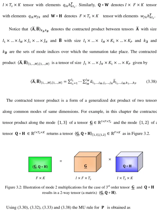
channels ( ) source separation ………... 33 Figure 3.2: Illustration of mode 2 multiplications for the case of 3rd order tensor
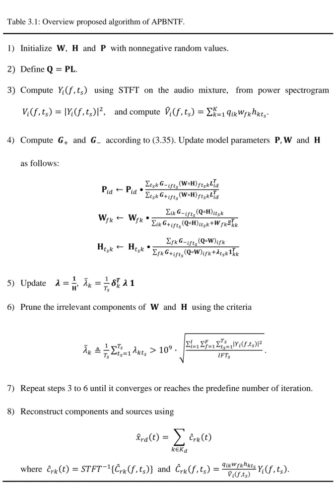
and results in a 2-way tensor (a matrix) ..……… 43 Figure 3.3: Real basis and code of the simulated mixed data……….. 48 Figure 3.4: Estimated results based on the proposed method without pruning and
without prior on ………. 49
Figure 3.5: Estimated results based on the proposed method with pruning and without
prior on ……….. 49
Figure 3.6: Estimated results based on adaptive sparsity factorization and with prior
on , i.e., ……….………….………. 49
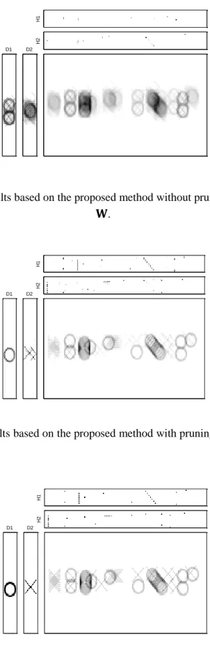
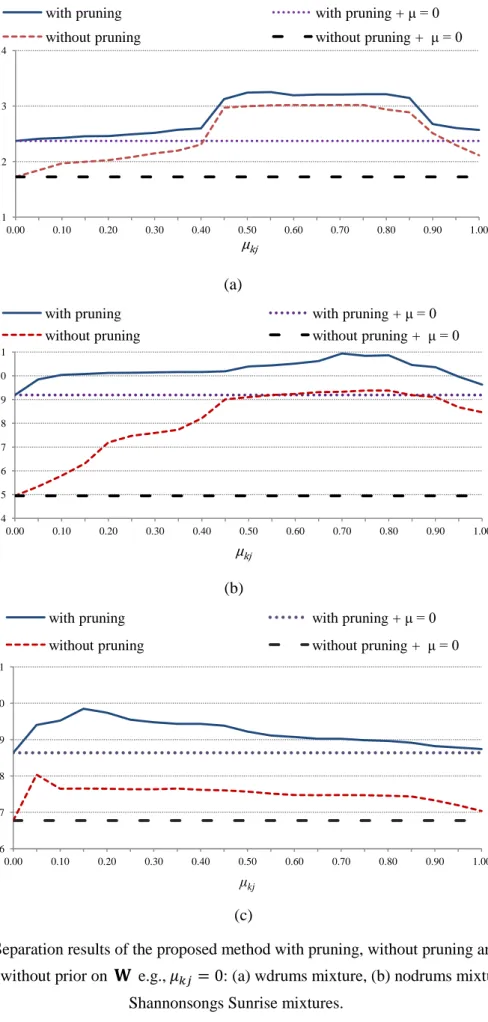
Figure 3.7: Separation results of the proposed method with pruning, without pruning and without pruning + without prior on e.g., : (a) wdrums
mixture, (b) nodrums mixtures, (c) Shannonsongs Sunrise mixtures……… 54 Figure 3.8: Original sources and the estimated sources from left microphone using the
proposed method with ……….
57 Figure 3.9: Time-domain representation of (a) the original source (Lead Guitar.) of
nodrums mixture, (b) and the estimated Lead Guitar from left microphone using the proposed method without pruning and (c) with pruning……….. 58 Figure 3.10: Time-domain representation of (a) the original sources (Bass) of
nodrums mixture ,(b) the estimated Bass signal from left microphone
Figure 3.11: Comparison of average SDR performance on wdrums, nodrums, and Shannonsongs Sunrise of three audio sources between IS-NTF, IS-cNTF, and the proposed method with per source and
……… (wdrums), (nodrums), (Shannonsongs Sunrise)…… 60
Figure 3.12: Comparison of average SDR performance on wdrums, nodrums, and Shannonsongs Sunrise of three audio sources between IS-NTF, IS-cNTF, and the proposed method with per source and
(wdrums), (nodrums), (Shannonsongs Sunrise)……. 61
Figure 3.13: Comparison of average SDR performance of estimated Hi-hat, Drum and Bass from wdrums dataset between IS-NTF, IS-cNTF, and proposed
method. .……… .……… 62
Figure 3.14: Separated signals of nodrums in time-domain. (a)-(c): original bass, Lead Guitar and Rhythmic Guitar music. (d)- (e): estimated sources using the proposed method (initial =3 and for all sources). (g)- (i): estimated sources using IS-cNTF. (j)- (l): estimated sources using
IS-NTF. (m)- (o): estimated sources using the proposed method (initial =20 and for bass, lead guitar and rhythmic
guitar, respectively)………. 63
Figure 4.1: Time-domain representation of the original sources, single channel mixture, and estimated sources of music mixture between piano and drum
using the proposed method..……….………. 84
Figure 4.2: TF domain representation of the original piano and drum music (top panels), mixed signal (middle panels), and separated signal piano and drum (bottom panels) using the proposed method ………. 84
Figure 4.3: Estimated . (a) piano (b) drum ……..………..………. 85
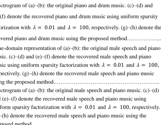
Figure 4.4: Overall separation results of different types of mixtures using the proposed method.………. ………….………….………….……….. 86 Figure 4.5: Time-domain representation of (a)–(b): the original piano and drum music. (c)–(d) and (e)–(f) denote the recovered piano and drum music using uniform sparsity factorization with and , respectively. (g)–(h) denote the recovered piano and drum music using the proposed
Figure 4.6: Spectrogram of (a)–(b): the original piano and drum music. (c)–(d) and (e)–(f) denote the recovered piano and drum music using uniform sparsity factorization with and , respectively. (g)–(h) denote the recovered piano and drum music using the proposed method….…………... 88 Figure 4.7: Time-domain representation of (a)–(b): the original male speech and piano
music. (c)–(d) and (e)–(f) denote the recovered male speech and piano music using uniform sparsity factorization with and , respectively. (g)–(h) denote the recovered male speech and piano music
using the proposed method.……….. 89
Figure 4.8: Spectrogram of (a)–(b): the original male speech and piano music. (c)–(d) and (e)–(f) denote the recovered male speech and piano music using uniform sparsity factorization with and , respectively. (g)–(h) denote the recovered male speech and piano music using the
proposed method….………..………. 90 Figure 4.9: Separation results of vL1-SCMF by using different uniform regularization... 93
Figure 5.1: The process of the proposed method for ………... 109
Figure 5.2: Original sources, single channel mixture, and estimated sources of music mixture between jazz and drum using the proposed method with
and .….….…………..…. ….….…………..….….….…………..…. 120 Figure 5.3: Comparison of average SDR performance on mixture of two audio sources
with SNMF2D, SCICA, and the proposed method with and 121 Figure 5.4: Original sources, single channel mixture, and estimated sources of
Shannonsongs Sunrise mixture using the proposed method with
and ….……....……….………...………… 122 Figure 5.5: Separation results of the proposed method by using different weight (
and time-delay parameters ….………..….………...….. 124
Figure 5.6: SDR results as a function of .(a) wdrums. (b) nodrums. (c)
LIST OF TABLES
Table 2.1: Algorithm of SCICA ………... 14
Table 2.2: Average SDR results for 3 types of mixtures in difference model N-HMM & N-FHMM and NMF.……….... 19
Table 3.1: Proposed APBNTF algorithm……….. 47
Table 3.2: Performance comparison between other NTF based multichannel audio source separation methods and the proposed method ………. 64 Table 3.3: Optimal number of and of wdrum, nodrum and Shannonsongs Sunrise ………... 66 Table 4.1: Overview the proposed vL1-SCMF algorithm ……… 82
Table 4.2: Comparison of average SDR and SIR performance on three types of mixtures between uniform regularization methods and the proposed method (vL1-SCMF)……….……….. 91 Table 4.3: Comparison of average SDR and SIR performance on three types of mixtures between SCICA, NMF-ISD, SNMF, CMF and the proposed method (vL1-SCMF)……….……….. 94 Table 5.1: Overview proposed algorithm of ISM-RNTF ………..… 117
Table 5.2: Comparison of average SDR, SIR and SAR performance on three mixtures between the proposed method, the proposed method without pruning, and the ISM-NTF ……….. 129
Table 5.3: Comparison of average SDR, SIR and SAR performance on three mixtures of three audio sources between SNMF2D, SCICA and the proposed method……….. 131
Table 6.1: Summary of the proposed BSS methods ……… 137
Table 6.2: Separation results using different SCBSS methods ……… 138
LIST OF SYMBOLS
the output from the multiplication of the compressed matrix weighted by the component of
the basis matrix
the weight matrix
where
Real positive number of rows F and columns T
the maximum number of sources
estimating the source which renders the better separation performance than a general
the channel number
The time slots the basis component
arbitrary set to be smaller than F and T an index of source
a non-negative data matrix
Z the number of basis
frequency bin time frame
the tensor with elements the tensor with elements
the tensor with elements
a multinomial distribution of frequencies for spectral component
a multinomial distribution of mixture weights at time frame
the magnitude spectrogram of sound source at time and frequency
The hidden state at time
the observed output at time
the state transition probability
the distribution of the observation given the state
an initial state distribution
the probability of all the observations
a multinomial distribution of frequencies
a multinomial distribution of the weights
the energy distribution
the observations across all time frames the number of draws over all time frames
the multivariate rectified Gaussian
a magnitude spectrum
phase spectra
the optimal parameters
a modeling error for each source
the multichannel audio mixtures
unknown sources
the source number
a mixing coefficient
the proper complex Gaussian distribution
a scalar cost function
the power spectrograms
equality up to constant
a certain “resemblance”
covariance matrix
modified multivariate Gaussian
the column vectorization
the multivariate Gaussian cumulative distribution function
the statistical expectation operator
the variance of the basis vector
the cross-covariance between and
the regularization parameter
the multivariate Gaussian cumulative distribution function
the negative part of the derivative of the criterion its positive part of the derivative of the criterion
threshold of the row of (equivalently column of )
actual source estimate interference signal
artifacts of the separation algorithm Complex number
Auxiliary function
The Gibbs distribution
the total number of source signals The weighted parameter
the time-delay
the maximum AR order
the th order AR coefficient of the th source signal at time
an independent identically distributed (i.i.d.) random signal with variance and zero mean
the mixing attenuation of the source
the residue of the source
the maximum time delay
the maximum frequency present in the sources
the sampling frequency
the STFT of
the STFT of
the STFT of
the selected minimum function of the channel a number of group of classified units a vector of activation coefficient
the tensor with coefficients
the estimated tensor with coefficients
the “labelling matrix” with only one nonzero value per column
a constant
the delta function
the statistical expectation operator
the cross-covariance between and
the estimated cross-covariance between and
the correlation between the basis vectors
The estimated correlation between the basis vectors
a Toeplitz matrix corresponding to the th diagonal sub-matrix of
where
exponentially decaying
the tensor with entries an element-wise product
a matrix
the smoothing parameter
the reconstructed source of the component in the channel the first-order correlation of
ABBREVIATIONS/ACRONYMS
2D
2-Dimensional
AIC
Akaike Information Criterion
APBNTF
Automatic Pruning
Bayesian
Non-negative Tensor
Factorization
AR
Autoregressive
ARD
Automatic Relevance Determination
ASR
Automatic/Automated Speech Recognition
BASS
Blind Audio Source Separation
BIC
Bayesian Information Criterion
BSS
Blind Source Separation
CASA
Computational Auditory Scene Analysis
CMF
Complex Matrix Factorization
cNTF
Cluster Non-negative Tensor Factorization
DUET
Degenerate Estimation Technique
EM
Expectation-Maximization
EEG
Electroencephalogram
HMM
Hidden Markov Model
ICA
Independent Component Analysis
ISM
Imitated Stereo Mixture
ISM-NTF
Imitated
Stereo
Mixture
non-negative
Tensor
Factorization
ISM-RNTF
Imitated Stereo Mixture Regularized non-negative Tensor
Factorization
KL
Kullback-Leibler
LS
Least Squares
MAP
Maximum A Posteriori
MEG
Magenetoencephalogram
ML
Maximum Likelihood
MSE
Mean - Square Error
MU
Multiplicative Update
N-HMM
Non-negative Hidden Markov Model
N-FHMM
Non-negative Factorial
Hidden Markov Model
NMF
Non-negative Matrix Factorization
NTF
Non-negative Tensor Factorization
PARAFAC
Parallel Factor Analysis
RWC
Real World Computing
SAR
Signal-to- Artifacts Ratio
SASS
Stereo Audio Source Separation
SC
Sparse Coding
SCICA
Single - Channel Independent Component Analysis
SCASS:
Single Channel Audio Source Separation
SDR
Signal-to-Distortion Ratio
SiSEC
Signal Separation Evaluation Campaign
SIR
Signal-to-Interference Ratio
SNMF
Sparse Non-negative Matrix Factorization
STFT
Short Time Fourier Transform
TF
Time Frequency
VB
Variational Bayesian
v
L1
-SCMF
Variational
L1
-Sparse Complex Matrix Factorization
LIST OF PUBLICATIONS
P. Parathai, W.L. Woo, and S.S. Dlay, “Monaural Blind Separation By Exploiting Source Temporal Correlation And Nonnegative Tensor Factorization Signal Processing”, accepted for Signal Processing
P. Parathai, W.L. Woo, and S.S. Dlay, “Single-Channel Blind Separation using
L1-Sparse Complex Nonnegative Matrix Factorization for Acoustic Signals” accepted
for Journal of the Acoustical Society of America
P. Parathai W.L. Woo, and S.S. Dlay, “Single-Channel Source Separation using Temporal Correlation with Regularized Nonnegative Tensor Factorization”, IEEE Transactions on Neural Networks and Learning System (under review)
P. Parathai, W.L. Woo, and S.S. Dlay, “MAP-based Regularized Nonnegative Tensor Factorization for Multichannel Source Separation,” IEEE Transactions on Audio, Speech and Language Processing (under review)
P. Parathai, W.L. Woo, and S.S. Dlay, “Single Channel Source Separation using Variational Lp-Sparse Complex Matrix Factorization”, IEEE Transactions on Neural
CHAPTER 1
INTRODUCTION TO THE THESIS
1.1 Background of Blind Source Separation
Humans are very good at focusing their attention on the speech of a single speaker, even in the presence of other speakers and background noise. One classical problem of blind source separation (BSS) [1] is the so-called “cocktail party problem” is a psychoacoustic phenomenon that refers to the remarkable human ability to selectively attend to and recognize one source of auditory input in a noisy environment, where the hearing interference is produced by competing speech sounds or a variety of noises that are often assumed to be independent of each other. Although the human brain and auditory system can handle this everyday problem with ease it is very hard to solve with computational algorithms. There are attempt to imitate the human performance with a machine by simplifying the complex perceptual task as a learning problem for tractable computational solution.
Speaker separation has conventionally been treated as a problem of Blind Source Separation. BSS [2] is an approach to unveil independent source signals from their mixtures without any prior information on the sources or the parameters of the mixed signal. Many methods for BSS have been proposed to reconstruct source signals for
example computational auditory scene analysis (CASA) relies on the development of a computational model of the auditory scene to automatically extract and track a sound signal of interest in a cocktail party environment, independent component analysis (ICA). ICA is a data driven method that makes good use of multiple inputs and relaxes the strong characteristic frequency structure assumptions.
The ICA algorithms find the independent components by maximizing the statistical independence of the estimated components. However, ICA algorithms perform best when the number of observed signals is greater than or equal to the number of sources [3]. BSS is broadly applied in different disciplines such as in order to deploy automatic speech recognition (ASR) effectively in real world scenarios it is necessary to handle hostile environments with multiple speech and noise sources. Current state-of-the-art ASR systems are trained on clean single talker speech and therefore inevitably have serious difficulties when confronted with noisy multi-talker environments [4].
Non-negative Matrix Factorization (NMF) has been ubiquitously used in many applications with great success for recovering underlying source signals given by a single sensor. The NMF method was invented by two scientists Lee and Seung [5] for factorizing a matrix into a product of two non-negative matrices. NMF has been applied extensively with considerable success to various problem domains, such as monaural sound source separation [6], polyphonic music transcription [7], face detection [8] and other signal-processing applications. NMF can project all signals that have the homogeneous spectral shape on a single basis, allowing one to represent a variety of phenomena efficiently using a very compact set of spectrum bases and there has been a
plenty of work in modeling audio using non-negative matrix factorization and its probabilistic counterparts as they yield rich models that are very useful for source separation and automatic music transcription. Learning time-varying spectra with standard NMF would require using a large number of basis vectors, and some post-processing to group the basis vectors into a single spectral vector. NMF and its extension are the prominent methods for linear combination that algorithms have been applied to solve the practical problems of BSS in many applications. Existing approaches have been successful in different conditions but none of them are yet satisfactory for speech application.
1.1.1 Blind Source Separation Problem using Nonnegative Matrix Factorization
Nonnegative matrix factorization (NMF) is an unsupervised data decomposition technique with considerable research success in the fields of blind source separation (BSS) [6, 9], data classification [10], data mining [11], pattern recognition [12], object detection [13], and dimensionality reduction [14]. Conventional NMF starts with a data matrix
with
. NMF factorizes this matrix into a product of two nonnegative matrices i.e. and such that
(1.1)
where F and T denote the total number of rows and columns in matrix , respectively. Generally, is arbitrary set to be smaller than F and T. Thus, matrix is the output
As such, the of is important for approximating the data in . Therefore, the matrix is considered as a set of basis vectors. NMF was initially developed using the multiplicative update (MU) algorithm to solve its parametric optimization based on the least square (LS) distance and Kullback-Liebler (KL) divergence as a cost function [15-16]. Other families of cost functions have been proposed, such as the Beta divergence [17], Csiszar’s divergences [18], and Itakura-Saito (IS) divergence [19]. Additionally, iterative gradient update was presented [20] and a sparseness constraint can be included into the cost function by regularization using the -norm based on minimizing penalized least squares [21] and using different sparsity constraints for and [22]. However, the sparsity parameter is manually determined the above proposed methods. Approximate sparsity is an important factor which represents significant information in . Many sparse solutions have been proposed in the last decade. Nonetheless, the optimal sparse solution remains an open issue.
1.1.2 Applications of BSS
BSS has been a hot topic in signal processing during last few decades. Applications of BSS have been reported in many fields. Such is the case when a sensor array records acoustic or electronic communications signals emanating from a number of different sources. BSS is an important technique used in applications such as a front-end for robust automatic speech recognition (ASR) where many proposed methods are based on independent component analysis (ICA). However, the performances of these methods degrade seriously particularly under extreme reverberant conditions. The experimental
results reveal that the separation performance of the ICA method proposed in [23, 24] using subarray processing is improved as the number of microphones is increased. An automatic music transcription task involves extracting information from individual sources. This task becomes more challenging when a given musical recording has numerous parts by numerous instruments. The one solution based on NMF approach [25] is to analyze frequency spectra of music signals and perform instrument separation or note transcription. If each of the instruments in the mixture can be modelled, they can be transcripted individually. This application is useful for a musician attempting to practice a particular instrument of interest directly from a multiinstrument recording.
Another example of the blind source separation application can be seen in medical applications where electrodes on the scalp record a mixture of signals generated by various sources of activity within the brain and are combined with sources of interference, such as signals generated by muscle activity. The BSS problem arises e.g. in analysis of the electric potentials on the scalp surface (electroencephalogram (EEG)), recording the magnetic fields near the surface of the head (magenetoencephalogram (MEG)). The analysis of the data is complex because it is possible that multiple neural generators are simultaneously active, and the potentials and magnetic fields from these sources overlap the footprint of the detectors [26]. In these cases, the BSS solution has been used to un-mix the data into signals representing the behaviors of the original individual generators. Recent research has also shown the feasibility of BSS techniques for various medical applications in [27, 28].
microphone array. In these cases, the use of multiple sensors array improves significantly the performance of the source separation algorithm. Microphones that should be used for robot audition given a specified array geometry i.e. the microphones are located around the robot’s head [29].
1.1.3 Blind Audio Source Separation
In this thesis, the special case of audio mixtures problem termed as blind channel source separation is focused. For blind audio source separation (BASS) methods, this denotes the separation of completely unknown sources without using additional training information. Most audio signals are mixtures of several audio sources (speech and music). This method consists in recovering one or several source signals from a given mixture signal. Figure 1.1 shows a general framework for BASS methods.
Figure 1.1: Overview of BASS approach.
Feature extraction Separation Signal Reconstruction Source estimate Audio mixture So ur ce sepa ra tio n p ha se
In Figure 1.1, the input to the separation system is only the audio mixture. The mixture is transformed into a suitable representation that directly through a signal reconstruction method to compute the estimates of the separated sources.
1.2 Objectives of Thesis
This thesis aims to investigate blind source separation methods in fundamental theories, assumptions, applications and limitations terms and further develop new algorithms of BSS for audio mixture. With this goal, the objectives are briefly explained in the following:
i). To present a unified perspective of the widely used state-of-the-art nonnegative matrix factorization (NMF) approaches. The theoretical aspects of BSS are presented to provide sufficient background knowledge relevant to the thesis.
ii). To develop rigorous new theories, mathematical derivations, and algorithms to recover the information about the original sources.
iii).To carry out analysis and comparisons of the proposed algorithms performance with state-of-the-art BSS methods by using objective as well as perceptual evaluation of audio quality using metrics such as the Signal-to-Distortion ratio (SDR).
1.3 Thesis Outline
Three novel methods based on NMF constitute the main contribution of the thesis. The thesis outline is as follows:
Chapter 2 provides an overview of recent source separation methods based on NMF approach is given. This chapter begins with an introduction to NMF methods and includes hidden Markov model (HMM) and complex components. The extention of NMF which is known as nonnegative tensor factorization (NTF) method is also reviewed.
Chapter 3 introduces a novel approach to Bayesian regularized cluster nonnegative tensor factorization under a parallel factor analysis
(
PARAFAC) structure. The basis for the proposed tensor factorization is developed under the framework of maximum aposteriori probability which is further adaptively fine-tuned using the hierarchical
Bayesian approach. This chapter will show that this method enables: 1) a generalized criterion for variable sparseness to be imposed onto each element of the temporal code; and 2) modified multivariate rectified Gaussian prior information to be explicitly incorporated into the basis features. This chapter also addresses the important issue of efficiency by using a framework of model selection for pruning unnecessary components and a novel Bayesian regularized cluster nonnegative tensor factorization under a PARAFAC structure with Itakura-Saito divergence. The proposed method is demonstrated further via experiments on underdetermined linear instantaneous stereo mixtures.
Chapter 4 covers a novel single-channel audio source separation (SCASS) which has been developed to extract better quality of audio separated signals. This chapter will introduce this approach that exploits the variational -sparse complex matrix factorization (v -SCMF) to offer the advantages of the CMF and a variational -sparse
approach, simultaneously and decomposes an information-bearing matrix into complex factor matrices that represent the spectral dictionary and temporal codes. The derivation of a variational Bayesian approach to compute the sparsity parameters for optimizing the matrix factorization will be presented. The method is then demonstrated on separating audio mixtures recorded from a single channel and its performance is compared with other existing sparse factorization methods. The performance of the developed algorithms will be measured using real-time audio signals in terms of the signal-to-distortion ratio.
Chapter 5 presents, a novel approach to solve the single-channel blind source separation (SCBSS) problem in which a new imitated-stereo mixture is formulated by weighting and time-shifting the original single-channel mixture. This chapter will show how paves the way to employ nonnegative tensor factorization applies to the monaural-channel problem by creating an artificial mixing system whose parameters can be estimated via a proposed nonnegative tensor factorization. The proposed tensor factorization is further developed under the framework of maximum a posteriori
probability and is adaptively fine-tuned under a PARAFAC structure with Itakura-Saito divergence. In addition, the separability analysis of the proposed imitated-stereo mixture is derived. Experimental testing on real-audio sources has been conducted to verify the capability of the proposed method.
1.4 Contribution
This thesis contributes three novel solutions for the BSS problem which can be summarised as follows:
i). A unified approach for the existing BSS methods based on nonnegative matrix factorization.
ii). A novel framework for multichannel blind source separation is proposed:
Unlike the conventional NTF approach, the proposed framework assigns a probability distribution to each element of and a sparsity parameter associated with each probability distribution. This sets up a platform to enable the sparsity parameter to be individually optimized for each element code.
It automatically detects the optimal number of components of the individual source (i.e. , where is the maximum number of sources). It designates a prior distribution on and determines the desirable in by pruning the irrelevant from . The term with the proper is used for estimating the source which renders the better separation performance than without the proper .
It incorporates prior information of the basis vectors using the modified multivariate rectified Gaussian. This benefits the overall algorithm in terms of better estimation accuracy and more meaningful feature extraction that pertain to the data. Since each pattern in the observed mixture has its own features,
designing the appropriate basis to match these features is imperative.
iii). A novel algorithm to solve SCBSS based on CMF is proposed.
Unlike the CMF, the proposed model is assigned a probability distribution to each element of and a sparsity parameter associated with each probability distribution. This sets up a platform to enable the sparsity parameter to be individually optimized for each element code.
The proposed algorithm enables the phase of constituent signals to be estimated more accurately for feature extraction. Since each pattern in has its own features, designing the appropriate phase to match these features is imperative. Incorporating the phase parameter will give the better recovered sources than without using phase information.
Each sparsity parameter in our model is learned and adapted as part of the matrix factorization.
iv). A novel method for single-channel blind source separation (SCBSS) based NTF is proposed.
The novel imitated-stereo mixture lights the way to reformulate NTF approaches into the single mixture. This relaxes the under-determined ill-conditions associated with monaural source separation.
The proposed solution separates sources from a single channel without relying on training information about the original sources.
CHAPTER 2
OVERVIEW OF BLIND SOURCE SEPARATION
The following sections will provide an overview of existing algorithms of the Single-channel Independent Component Analysis (SCICA), nonnegative matrix factorization (NMF) composed of single channel NMF [30-32] and multi-channel NMF which is known as Nonnegative Tensor Factorization (NTF). NTF is a multidimensional model with nonnegativity constraints. Generally, the term ‘tensor’ denotes multi-way arrays and the order of a tensor is the number of modes, also known as ways or dimensions. The details of these approaches are discussed in Sections 2.1, 2.2 and 2.3.
2.1Single-channel Independent Component Analysis
The ICA-based methods [33 - 35] show very successful, and perhaps, the most widely used, for performing blind source separation in the general case. Single-channel independent component analysis (SCICA) is a BSS technique that extracts statistically independent sources from a single-channel recording. SCICA is an adaptation of the standard ICA algorithm to one observed sensor, which has already been proposed in [24, 36, 37]. The mixtures can then be separated by only employing the standard ICA. The observation model is expressed as:
(2.1) where the matrix is an unknown constant matrix called the mixing coefficient
matrix. The task is to identify the mixing coefficient matrix , and separate the source signals while only knowing a sample of observed vectors . The term represents independent signals. Generally, the original signals can be separated from as shown in the following:
where (2.2)
For SCICA, the observed mixture is broken up into a sequence of contiguous blocks with length . These are treated as a sequence of vector mixtures:
(2.3)
where is the block index is a time delay, and is the length of the original signal. The matrix is then formed as a set of mixtures as the following:
(2.4)
The FastICA algorithm [38-40] can then be applied to to compute the mixing and unmixing matrix and . For a perfect reconstruction decomposition, the separation process must be performed in the mixture domain where each signal is discovered via and as:
(2.5)
where is the original signal in the mixture domain i.e. . The signal is consecutively estimated and subtracted from one at a time where the
extract the second signal and so on which is presented in Table 2.1.
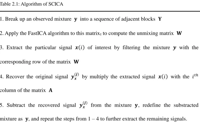
Table 2.1: Algorithm of SCICA
1. Break up an observed mixture into a sequence of adjacent blocks
2. Apply the FastICA algorithm to this matrix, to compute the unmixing matrix 3. Extract the particular signal of interest by filtering the mixture with the corresponding row of the matrix
4. Recover the original signal by multiply the extracted signal with the column of the matrix
5. Subtract the recovered signal from the mixture , redefine the substracted mixture as , and repeat the steps from 1 – 4 to further extract the remaining signals.
However, SCICA has two major drawbacks: first, the algorithm assumes stationary sources, and second, the sources are assumed to be disjoint in the frequency domain.
2.2Nonnegative Matrix Factorization Approaches
In recent years, there is growing interest in the field of BSS using factorization-based approaches [41–45]. Non-Negative Matrix factorization (NMF) is a data-adaptive linear representation method for 2-D matrices as presented in Figure 2.1. NMF decomposes a non-negative data matrix into the product of two non-negative matrix factors and
:
Figure 2.1: Diagrame of NMF
Where plays the role of the basic matrix, while represents the weight matrix. The parameter indicates the number of basis used to represent the original matrix. The basis can be considered as spectral patterns which are frequently observed. NMF is an additive model which does not allow subtraction. To find such a pair of and which minimizes the error of the approximation in (2.6), two alternative cost functions are defined: Euclidean distance, , and Divergence, :
(2.7)
(2.8)
NMF aims to calculate the factor of the matrix in the form of the product of matrix . is any positive integer which is less than or [46] chosen for finding components. For the problem of sound separation at any position, of the matrix is the amplitude of each frequency at different time when and
presented in spectrogram as shown in (2.6) and can be explained by using linear
algebra. Figure 2.1 shows the matrix as column vector of length F with T vectors. The columns of consists of F-dimensional data vectors. The columns of contains basis vectors of dimension F. Each T-dimensional column vector of the approximation as (2.6) is a linear combination of all basis vectors, whereby the coefficients are the entries of the corresponding Z-dimensional column vector of .
After estimating the matrix and in a source separation, the next step is to select only the basis vector of the sound source from both of the matrices such as column at and row at of the matrix and respectively. Next, multiplication of and yields a new matrix size F× T to be used in calculating the spectrum of the target sound with various methods to follow.
Thus, NMF algorithms aim to find a local minimum of the divergences. Commonly used cost functions for NMF are the generalized Kullback-Leibler (KL) divergence and Least Square (LS) distance which have been introduced in [5], respectively, as:
(2.9) where is the power TF representation of mixture which can be further factorized as the product of two nonnegative matrices and and . From the above equations, is equivalent to an assumed Poisson noise model for the data and is equivalent to the maximum likelihood estimation of and in additive independent and identically distributed (i.i.d.) Gaussian noise. The widely used estimation
algorithms of Lee and Seung [5] minimize the chosen cost function by initializing the entries of and with random positive values, and then update those iteratively using multiplicative rules. Each update decreases the value of the cost function until the algorithm converges. The update rule for KL divergence is given by:
(2.10)
and
(2.11)
where ‘ ’ and ‘ ’ denote the element-wise product multiplication and division, respectively. ‘ ’ is an all-one by matrix. The update rule for LS distance is given by:
(2.12) and
(2.13)
On the one hand, the following are advantages of NMF: The mixing model is defined in the magnitude spectrum domain. Because of the phase-invariant nature of magnitude spectra, NMF is able to project all signals that have the same spectral shape onto a single basis. This allows us to represent a variety of acoustic phenomena efficiently using a very compact set of spectrum bases. On the other hand, NMF cannot estimate the phase spectra of underlying constituent signals, which certainly limits its range of applications.
2.2.1 NMF using Hidden Markov Model
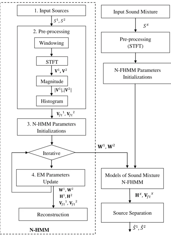
Figure 2.2: Overview of N-HMM method.
This section presents a model of single source sounds, Non-negative hidden Markov model (N-HMM) [47], which combines the rich spectral representative power of NMF
1. Input Sources 3. N-HMM Parameters Initializations 2. Pre-processing Source Separation 4. EM Parameters Update
Models of Sound Mixture N-FHMM
Iterative
Input Sound Mixture
N-FHMM Parameters Initializations Pre-processing (STFT) STFT Magnitude Histogram , , , , , , , N-HMM Windowing Reconstruction , ,
and the temporal structure modeling of traditional HMMs [48]. The overview of the N-HMM method is presented in Figure 2.2. N-HMM is consistent with the non-stationary nature of audio as a multiple learning small dictionaries of spectral components to describe different features of the sound source. Furthermore, it can be used to model the temporal dynamics of the sound source between dictionaries by learning a Markov chain.
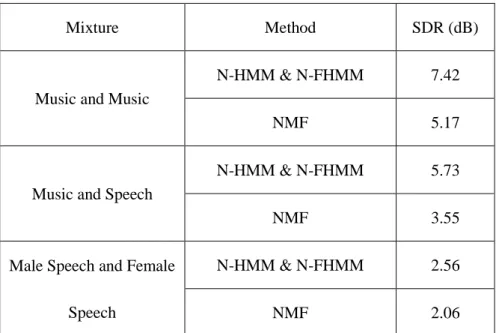
Table 2.2 Average SDR results for 3 types of mixtures in difference model N-HMM & N-FHMM and NMF.
Mixture Method SDR (dB)
Music and Music
N-HMM & N-FHMM 7.42
NMF 5.17
Music and Speech
N-HMM & N-FHMM 5.73
NMF 3.55
Male Speech and Female Speech
N-HMM & N-FHMM 2.56
NMF 2.06
The overall comparison results between the N-HMM & N-FHMM and NMF methods have been summarized in Table 2.2. According to the table, the N-HMM& N-FHMM tends to yield better result than NMF method. The average performance improvement of the N-HMM& N-FHMM method against the NMF method: 1) for the music and music mixtures, the improvement SDR per source is 2.25dB. 2) For the music and speech mixtures, the improvement per source in term of SDR is 2.18dB. 3) For the male speech
The results demonstrate that this approach is applicable to model the individual sources by learning several small dictionaries using NMF method and a Markov chain. Sources have been modeled via HMM in time-frequency domain obtain prior information of the original signals. Good separation performance with high SDR has been obtained using the method. However, the mixing model implicitly assumes the added magnitude spectra which only approximately hold, although attempts are made to mitigate the non-additive problem with respect to NMF. NMF cannot estimate the phase spectra of underlying constituent signals, which certainly limits its range of applications. Moreover, the phase coherence between frequency components can be easily destroyed as a result of many factors. It is difficult to capture high-level structural elements from observations through the use of complex-spectrum bases.
2.2.2 Bayesian Non-negative Matrix Factorization
Bayesian NMF [49] assumes a Gaussian likelihood, independent exponential priors on and with scales , and derive an efficient Gibbs sampler to approximate the posterior density of the NMF factors. It is assumed that the residuals are i.i.d. zero mean normal with variance , which gives rise to the likelihood
(2.14)
(2.15) and
where θ = { , } denotes all parameters in the model. The prior for the noise variance is chosen as an inverse gamma density with shape and scale ,
(2.17)
According to Bayes' rule, the posterior distribution of all parameters in the model is given by
(2.18) The joint posterior density is approximated in a sampling scheme by iteratively sampling one parameter while keeping all others fixed. Expressions are derived for the conditional posterior densities of the model parameters
(2.19)
(2.20)
and (2.21)
where the index –f,k depicts all entries of a matrix except entry f,k.
A Gibbs sampler is used to maximize the posterior density of the parameters by iteratively drawing samples from these conditional posterior distributions which converge towards the joint posterior distribution. Fortunately, there are closed forms of the densities to be drawn from and hence no samples need to be stored and the normalization constant can be computed. The authors demonstrate that the procedure is able to determine the correct number of components in a toy example and in a chemical shift
2.2.3 NMF with Automatic Relevance Determinant
In [62] presented automatic relevance determination for KL-NMF for model order selection which does not need to evaluate the evidence by formulating a MAP criterion:
(2.22) using KL-divergence log likelihood and independent half-normal priors on each column of and row of with precision parameter
(2.23)
(2.24)
The precision parameters are provided with a Gamma prior
(2.25)
with fixed hyperparameters and .
A multiplicative algorithm optimizes in (2.22) by iteratively updating , and . The data automatically determines the optimal values of the hyperparameters . The algorithm is initialized with a relatively large value of components and successively drives unnecessary components to extinction. This property results from Bayesian inference: a subset of the precision parameters will be driven to an upper bound which corresponds to a sharp peak at zero for the priors on and row and leads to an effective extinction of column and row . The effective number of components is determined by the number parameters which are not driven to an upper bound during the iterations.
2.3 Complex Non-negative Matrix Factorization
This section presents a mixture model defined in the complex time-frequency domain. Complex Non-Negative Matrix Factorization model (CMF) [50-52, 80] is a sparse representation for acoustic signals which offers the advantages of the sparse coding (SC) [81-83] and non-negative matrix factorization (NMF) [5] concurrently. It can extract the recurrent patterns of magnitude spectra and the phase estimates of constituent signals, and can be performed with an efficient iterative algorithm. CMF shares with NMF the ability to generate non-negative matrices and , while the input matrix is assumed to be a complex matrix and the algorithm also generates a third-rank complex-valued tensor as the following
(2.26)
It is assumed that the short-time Fourier transform (STFT) of an audio signal, in frequency bin and time frame , is composed of complex-valued elements
(2.27)
Each is assumed to have a magnitude spectrum which is constant up to the gain over time:
(2.28)
and a time-varying phase spectrum
The CMF model can be expressed as
(2.30)
where corresponds to recurring magnitude spectral pattern, to time-varying activation coefficients and to time-varying phase spectra and assume
(2.31)
in order to eliminate an indeterminacy in the scaling between and .
The CMF method in [50] can be summarized as follows:
(1) Transform the single channel mixture of two sources: form the time domain to the time-frequency domain using STFT.
(2) Initialize and . (3) Update
.
(4) Stabilize the algorithm by running NMF at the beginning of the iteration, which can be performed simply by fixing the value of at
. (5) The iterative algorithm is summarized as follows:
1. Update by computing , and . 2. Update by computing , , and .
(6) Obtain the estimation of each source 1 and 2 by applying two different
methods
(6.1) Atom selection method
The magnitude of atomic spectrum closest to the true spectrum was selected for each frame, and the framewise signals, each of which constructed using the selected atom and the corresponding activation coefficient and phase spectrum, were concatenated to synthesize the whole signal stream [50].
(6.2) Reconstruction
The reconstruction is calculated by multiplying the row of the spectral components
with the corresponding column of the mixture weights and time-varying phrase spectrum . Then, convert the time-frequency represented sources back into time domain.
An experimental results of the CMF method showed that reasonably good separation performance on the single-channel audio source separation can be obtained.
2.4 Nonnegative Tensor Factorization Approach
In this case, the extension of NMF for solving multichannel mixtures has been regarded by stacking up the spectrograms of each channel into a single matrix [53]. This approach is considered as nonnegative tensor factorization (NTF), also called nonnegative parallel factor analysis (PARAFAC), where the channel spectrograms are jointly modeled by a 3-valence tensor [54]. NTF was introduced by Shashua and Hazan in [55] and has
become a popular technique for data analysis and dimensionality reduction, parts-based representation of nonnegative data. Algorithms for NTF such as PARAFAC have been used for audio source separation in [54, 56]. Regardless of the cost function used, in order to achieve audio source separation, some methods require grouping of the basis functions according to the sources or instruments. Different grouping methods have been proposed by Casey [57] and Virtanen [6], but in practice, if the sources overlap in the time-frequency (TF) domain, it is difficult to obtain the correct clustering. This issue is discussed in [58]. Clustering of the spatial cues to group the NTF components (cNTF) [56] was developed for multichannel audio source separation. In most applications, it is crucial that the “right” model order is selected. If is too small, the data does not fit the model well. Conversely, if is too large, then overfitting occurs. It is aimed to find an elegant solution for this dichotomy between data fidelity and overfitting. Choosing the right model is in particular challenging in the PARAFAC model as the number of components is specified for each modality separately. This delivers heuristics such as the Bayesian information criterion (BIC) [59] and Akaike information criterion (AIC) [60].
Both techniques cannot account for additional constraints such as non-negativity. Furthermore, a Bayesian approach of automatic relevance determination (ARD) was introduced by Mackay [61] to determine the relevant number of explanatory variables in the context of regression. This technique was used in [62 - 64] based on NMF model and multi-way models as in [65]. The spectral dictionary obtained via NMF-ARD [66] methods is not adequate to capture the temporal dependency of the frequency patterns within the audio signal. In addition, the NMF-ARD does not model musical notes but
rather unique events only. Thus, if two notes are always played simultaneously they will be modeled as one component. Also, some components might not correspond to notes but rather to the model, e.g., background noise.
Nonnegative tensor factorization (NTF) has been proven to be a very useful tool in a variety of signal processing fields. Recently, NTF methods have successfully been exploited for data mining, dimensionality reduction, pattern recognition, object detection, gene clustering, sparse nonnegative representation and coding, and blind source separation (BSS) [67–75].
Given a data tensor and the positive index , the goal is to find three-component matrices, also called loading matrices, ,
and which performs the following approximate factorization. is the tensor with coefficient
and is estimated tensor with coefficient
. The NTF under PARAFAC structure can be formulated in the element-wise form as follows
(2.32)
A PARAFAC model is given by the matrices of , , and with elements , and , respectively. The trilinear model is found to minimize the sum of squares of the residuals, in the model. Figure 2.3 illustrates the principle of the PARAFAC model.
Figure 2.3: A graphical representation the principle of the decomposition of a 3-way data cube according to the PARAFAC model.
2.5 Summary
The state-of the art blind source separation method have been explained in this chapter. Generally speaking, more sparseness of the constructing components yields the better approximation. The NMF method is a flexible approach which can be developed as a new cost function, sparsity updating, and a new factorization for quantity analyzing of data to render better separation performance. Solving the BSS problem by using NMF approach has drawn huge interest from researchers in last two decades. However, the qualities of the reconstructed sources are not enough to launch the NMF solution in a real application.
CHAPTER 3
MAP-BASED REGULARIZED NONNEGATIVE TENSOR
FACTORIZATION FOR MULTICHANNEL SOURCE SEPARATION
In this chapter, a novel approach to Bayesian regularized cluster nonnegative tensor factorization under a PARAFAC structure is presented. The proposed tensor factorization is developed under the framework of maximum a posteriori probability and is adaptively fine-tuned using the hierarchical Bayesian approach. The method enables: 1) a generalized criterion for variable sparseness to be imposed onto each element of the temporal code; and 2) modified multivariate rectified Gaussian prior information to be explicitly incorporated into the basis features. Underlying all factorization algorithms is the principal difficulty in estimating the adequate number of latent components for each source.This method takes the advantage of the combination of the automatic detection of the optimal through both the pruning technique and the prior information on to estimate the signature parameter of the original sources. This chapter addresses this important issue by using a framework of model selection for pruning unnecessary components and a novel Bayesian regularized cluster nonnegative tensor factorization under a PARAFAC structure with Itakura-Saito divergence. The experiments were designed to demonstrate on underdetermined linear instantaneous stereo mixtures of musical sources. The proposed method gives an average performance improvement of at
least twice better than the state-of-art Itakura-Saito Nonnegative Tensor Factorization (IS-NTF) and Itakura-Saito with Cluster Nonnegative Tensor Factorization (IS-cNTF) methods, respectively.
The chapter is organized as follows: Section 3.1 introduces the background of NTF with IS Divergence. Section 3.2 describes the generative model of the proposed method, and the formulation of the NTF algorithm. Experimental results with a series of performance comparison with other NTF techniques are presented in Section 3.3. Finally, Section 3.4 concludes the chapter.
3.1 Background
3.1.1 NTF with Itakura-Saito Divergence
A statistical IS-NTF model of the observation can be expressed as
(3.1)
where is defined as if and only if . The corresponds to mixing coefficient in a mixing matrix. The components will be characterized by a spectral shape and a vector of activation coefficient through a statistical model and
(3.2)
where denotes the proper complex Gaussian distribution and is the variance.
The factorization [15] is usually achieved through the minimization problem
(3.3)
where is a scalar cost function.
In this section, the term is exploited to be the IS divergence whichis defined as [19]
(3.4)
Thus, log-likelihood of the factor , and can be written as
(3.5)
where is the matrix with entries and “ ” denotes equality up to constant.
3.2 Proposed APBNTF Method 3.2.1 Generative Model
Under the linear instantaneous mixing and the point-sources assumption, the multichannel audio mixtures can be generated by several unknown sources