Partition-based clustering using constraint optimization

Optimization

Valerio Grossi, Tias Guns, Anna Monreale, Mirco Nanni, and Siegfried Nijssen

Abstract Partition-based clustering is the task of partitioning a dataset in a number of groups of examples, such that examples in each group are similar to each other. Many criteria for what constitutes a good clustering have been identified in the liter-ature; furthermore, the use of additional constraints to find more useful clusterings has been proposed. In this chapter, it will be shown that most of these clustering tasks can be formalized using optimization criteria and constraints. We demonstrate how a range of clustering tasks can be modelled in generic constraint programming languages with these constraints and optimization criteria. Using the constraint-based modeling approach we also relate the DBSCAN method for density-constraint-based clustering to the label propagation technique for community discovery.

1 Introduction

Clustering [15] is the data analysis task of grouping sets of object. It is an unsu-pervised task, meaning that no information is known about the true grouping of the objects. In general, the goal is to find clusters whose objects are similar to each other

Valerio Grossi·Anna Monreale

University of Pisa, Largo B. Pontecorvo, 3 56127 Pisa; e-mail: [email protected], [email protected]

Mirco Nanni

ISTI - CNR, Via Moruzzi, 1, 56124 Pisa, Italy e-mail: [email protected] Tias Guns·Siegfried Nijssen

Department of computer science, KU Leuven, Celestijnenlaan 200A, 3001 Leuven, Belgium; e-mail: [email protected]

Siegfried Nijssen

Leiden Institute for Advanced Computer Science (LIACS), Niels Bohrweg 1, 2333CA Leiden, The Netherlands; e-mail: [email protected]

while different from the objects in the other clusters. Clustering can lead to better insights into data and to discoveries of previously unknown groupings.

Many different clustering settings have been studied in the literature. The focus of this chapter is on partition-based clustering. In partition-based clustering, the clustering must form a partition, that is, each object can only belong to one cluster. This is in contrast to for instance hierarchical clustering, where clusters form a tree in which one cluster can be a subset of another cluster.

An important aspect in partition-based clustering is the scoring function that is used to determine the quality of a clustering. In the literature many different methods for calculating the quality of a clustering have been proposed. A range of popular partition-based methods are based on the concept of a clusterprototype. Prototype-based techniques evaluate clusters Prototype-based on the distance of points in the cluster to the prototype. These approaches provide clusters having spherical shapes. Other approaches consider the diameter of the clusters, or their distance to other clusters. Density-based techniques (e.g. DBSCAN) discover clusters of any shape, and are designed for discovering dense areas surrounded by areas with low density, typically formed by noise or outliers.

Another aspect of clustering methods is which constraints they support. Con-straints can be used to specify additional requirements on the clusters that need to be found. The most well-known of such requirements are themust-linkand cannot-linkconstraints, which specify that certain data points should or may not be clustered together [18, 3].

In this chapter, we will show that many of these clustering problems can be for-malized as generic constraint optimization problems. Consequently, generic con-straint optimization solvers can be used to address a wide range of clustering prob-lems. One motivation for the use of generic constraint optimization techniques in this context is the large number of choices that need to be made in defining a clus-tering setting. Central questions are here:

• how do we define the coherence of a cluster?

• how do we define the number of clusters that we wish to find? • what other properties must the clusters satisfy?

While such constraints and optimization criteria may sometimes be added in spe-cialized techniques, generic techniques that allow for the specification of such con-straints and optimiation criteria would be applicable more widely.

Within this chapter, we will distinguish two types of partitioning-based clustering settings:direct andindirectmethods. These settings differ in how the number of clusters is determined. Thedirectmethods require that a user specifies the number of clusters explicitly by setting a parameterk, which can be interpreted as a constraint on the number of clusters. Forindirectmethods, the number of clusters is indirectly specified through constraints on the coherence of a cluster; more clusters are created if a smaller number of clusters would not be sufficiently coherent [1].

We first discuss the direct approaches based on a parameterk(Section 2), fol-lowed by the indirect approaches (Section 3). Here, Section 2 first introduces sev-eral optimization criteria and then outlines common user-specified constraints in

clustering. Different modeling choices are presented and demonstrated on a range of clustering problems.

The section on indirect approaches (Section 2) shows how clusters can also be modeled as separated regions of high data density. This corresponds to the princi-ple behind theDBSCANalgorithm. Furthermore, we draw a link between this data clustering task and the mechanism ofLabel Propagationas used in community de-tection in graphs.

2 Direct Methods

Characteristic for direct methods is that users need to specify the number of clusters in advance by means of a parameterk. These methods will subsequently focus on finding a good clustering with this number of clusters.

Of crucial importance is then how to evaluate the quality of one cluster. Here, several approaches are possible.

The most studied and applied approaches are those in which a cluster prototype is identified. Every cluster is represented by a prototype called thecentroidof the clus-ter. Two popular algorithms employing this approach areK-meansandK-medoids. In K-means each centroid represents the average of all points in the cluster, while in K-medoids the centroid is the most representative actual point in the cluster.

Other approaches do not identify an explicit prototype, but evaluate all pairwise distances between points in the cluster, or evaluate the pairwise distances between points inside and outside the cluster.

From an algorithmic perspective, most algorithms for finding clusters are heuris-tic. K-means and K-medoids are good examples. Given a user-specified value k, these algorithms selectk initial centroids. Successively each point is assigned to the closest centroid based on a distance measure. Finally, the centroids are updated iteratively based on the points assigned to the clusters. This process stops when centroids do not change.

In this chapter, we take a step back from this algorithmic view and look at the un-derlying optimisation problems that clustering methods are trying to solve. We first describe the different optimization criteria that can be used, followed by constraints that can be put on clusters or the entire clusterings.

In the following, we assume given a set of data pointsDof sizen. Each point p is represented by anm-dimensional vector. A clusterCis a set of points:C⊆D, and a clusteringC is a partitioning of the data into clusters:∀C∈C :C⊆D,S

C∈CC= D,∀C1,C2∈C:C1∩C2=/0. Note that we consider non-overlapping clusters here.

2.1 Optimization Criteria

Intuitively, a clustering consists of clusters that are coherent and whose data points are similar to each other; on the other hand we also expect the clusters (and data points therein) to not be similar to the other clusters [15].

There are many different ways to characterize how good a clustering is, by mea-suring the (dis)similarity of its clusters and data points. We identify a number of these measures below. Each measure can be used as an optimisation criterium to find a ‘good’ clustering according to this measure.

Sum of squared inter-cluster distances.Given some distance functiond(·,·)over points, for example, the Euclidean distance, we can measure the sum of squared distances within each cluster as follows:

∑

C∈C p,q∈

∑

C,p<q

d2(p,q) (1)

Here we assume that p<qiff data point pis before pointqin the database; this ensures that every pair of points is considered only once.

Sum of squared error to centroid.A more common approach is to measure the “error” of each cluster, that is, the distance of each point in the cluster to the mean (centroid) of that cluster.

We compute thecentroidof a cluster by computing the mean of the data points that belong to it:

zC=mean(C) =∑p∈Cp

|C| (2)

Here, we assume that the points pare represented as vectors and traditional vector algebra is used. The sum of squared error is then measured as:

∑

C∈C p

∑

∈C

d2(p,zC) (3)

Note that this is identical to the sum of all pairwise distances between the points of a cluster, divided by the size of that cluster:∑C∈C∑p,q∈C,p<qd2(p,q)/|C|.

Sum of squared error to medoids. Instead of using the mean (centroid) of the cluster, one can also use the medoid of the cluster, that is, the point that is most representative of the cluster. Let the medoid of a cluster be the point with smallest average distance to the other points:

yC=medoid(C) =arg min y∈C_p

∑

_∈Cd

2_{(p,y). (4)}

∑

C∈C p

∑

∈C

d2(p,yC) (5)

Cluster diameter.Another measure of coherence is to measure the diameter of the largest cluster, where the diameter is defined as the largest distance between any two points of a cluster. This leads to the following measure of maximum cluster diameter:

max

C∈C p,qmax∈C,p<qd(p,q) (6) One can imagine other variants such as the sum of diameters.

Inter-cluster margin. The margin between two clusters is the minimal distance between any two points that belong to the different clusters. The margin gives an indication of how different the clusters are from each other (e.g. how far apart they are). This can be optimized using the following measure of minimum inter-cluster margin:

min

C,D∈C p∈minC,q∈Dd(p,q) (7)

2.2 Constraints

Using constraints for defining data mining tasks guarantees a high level of expres-sivity, since adding new constraints on the required output is quite easy and natu-ral. Constraints typically specify background knowledge that the user has about the clustering. A famous example [18] is that clusters should group cars in lanes, and hence one can derive that some objects can certainly not be in the same cluster (e.g. when known to be driving side-by-side) while others certainly are (when driving in tandem).

The above example is an illustration of instance-levelconstraints, that is, con-straints between specific points. Must-linkconstraints require that two points be-long to the same cluster, whileCannot-linkconstraints require that two points be-long to different clusters [18]. AMust-linkconstraint on two points pandqis ex-pressed by:∀C∈C :p∈C↔q∈C; while aCannot-link constraint is expressed by:∀C∈C :p∈C→q∈/C.

Another type of constraints iscluster-level constraints [9]. Theε-constraint or

maximal diameter constraint requires that the diameter of a cluster is at mostε, that

is, each two points in a cluster are at mostε apart. This can also be formulated as

requiring that each pair of points pandqthat is further apart cannot be together in the same cluster:∀p,q: d(p,q)>ε→(∀C∈C :p∈C→q∈/C). Theδ-constraint

or minimal margin constraint requires that two points belonging to different clusters have to be at leastδ apart. Alternatively formulated: any two points that are closer

thanδ must belong to the same cluster:∀p,q: d(p,q)<δ →(∀C∈C :p∈C↔

q∈C).

Other user-defined constraints can be expressed [7]. One can impose constraint on the clusterssize, e.g. requiring clusters with a minimum or maximum number of points. Constraining the number of points to be minimum or maximum α is

expressed as:∀C∈C :|C| ≥αand∀C∈C :|C| ≤α.

Furthermore, any of the measures introduced in the previous section on opti-mization criteria can also be constrained to take a value within a certain interval. Other variants and combinations of these constraints can be employed as well, such as disjunctions of constraints or conditional must-link and cannot-link constraints. One can add constraints that certain individual clusters must be similar or different from predefined sets of points, or addsoftconstraints such as a bound on the number of points that can have a cannot-link constraint [2].

The complexity of adding constraints to (k-means) clustering has been studied in [10]. A general overview of constraint-based methods in clustering is available in the book ”Constrained Clustering: Advances in Algorithms, Theory, and Applica-tions” [3]. Furthermore, the chapter “Data Mining & Constraints: an Overview” of this book provides several references to using constraints in data mining tasks also for clustering.

2.3 Modeling clustering as constraint optimization

A constraint optimization problemP= (V,D,X,f)consists of variablesV, a domain Dthat lists the possible values the variables can take, a set of constraintsX overV and an optimization function f overVthat must be minimized or maximized.

Building on the primitives introduced earlier, many well-known clustering prob-lems can now be modelled as follows, for a given optimization criterionquality(C):

maximizeC quality(C), (8) s.t. C1∩C2=/0 ∀C1,C2∈C (9) |[ C∈C C|=n (10) |_C|=k (11)

Heren is the total number of points. In this setting, the number of clusters to be found is fixed and has to bek.

Note that the model above uses a set notation for the clusters. Not all constraint solvers support sets; set variables may not always be the most efficient representa-tion either. For these reasons, anencodingof the sets in variables of other types is sometimes necessary. There are various ways to model these sets, as well as differ-ent solving techniques that can be used on these models. We differdiffer-entiate between three kinds of approaches:

• Constraint formulations that can directly be solved by most state-of-the-art con-straint programming systems;

• Formulations that require an extension of a Constraint Programming system; • Hybrid approaches with a specialized system that can deal with a range of

clus-tering problems, but no other problems.

We will discuss these possibilities in more detail below.

2.3.1 Constraint solving formulations

To use constraint programming systems off-the-shelf, an important question that needs to be answered is how to encode a clustering in such systems. Next to a set-based notation, several representations have been proposed. We will use these representations to construct clustering models in the next section:

• a Boolean representation, in which a variableaitwith domain{0,1}takes value 1 iff pointi(with 1≤i≤n) is in clustert (with 1≤t≤k), and takes value 0 otherwise. Constraints

k

∑

t=1

ait=1

for all pointsiensure that a point is in only one cluster [14];

• a Boolean representation, in which a variableatwith domain{0,1}takes value 1 iff possible clustert(with 1≤t≤2n_{, i.e. each possible cluster is given an index)} is in the clustering; constraint∑2

n

t=1at=kensures exactlykpossible clusters are selected and constraints

2n

∑

t=1

[i∈Ct]at=1

ensure that every pointiis in exactly one chosen cluster; here[i∈Ct]is an indi-cator that takes value 1 iff pointiis in possible clustert[16, 11];

• an integer representation, in which a variableaiwith domain{1, . . . ,k}indicates that pointi(with 1≤i≤n) is in clusterai[8];

• an integer representation, in which a variablegiwith domain{1, . . . ,n}identifies the point with the smallest index that is in the same cluster as pointi; note that gi=iiff there is no point j<iin the same cluster as pointi[7].

An important benefit of the first Boolean representation is that it is easy to formalize additional constraints in this representation. AMust-linkconstraint on two pointspi andpjis expressed by a set ofait=ajt constraints, where 1≤t≤k; acannot-link constraint is expressed by:∀t∈ {1, . . . ,k}:ait+ajt ≤1. Asizeconstraint can be expressed by: ∀t∈ {1, . . . ,k}: n

∑

i=1 ait≥α ∀t∈ {1, . . . ,k}: n

∑

i=1 ait≤α.

A drawback of this representation is that additional constraints are required to ensure that a point is not in two clusters; this is not necessary in the integer repre-sentations.

The second Boolean representation has as most important drawback that its num-ber of variables is very large. One way to address this is to limit the numnum-ber of possible clusters apriori; ideas for this were presented in [16].

The main difference between the integer representations is that in the second rep-resentation the indexes of representative points are used to identify clusters, while in the first cluster indexes are used. In the second representation the number of clus-ters is not fixed; to achieve a fixed number of clusclus-ters, additional variablescjwith domain{1, . . . ,n}, where 1≤j≤k, can be used, with the constraints:

• gcj=cjfor all clusters j, i.e., variablecjpoints to the identifying point for each

cluster;

• ∑k_j=1[gi=cj] =1 for each pointi; this ensures that each pointialso belongs to one of thekclusters identified byc.

A remaining challenge is how to represent the optimization criterion. In many cases, additional variables are needed. This is illustrated for a number of cases be-low.

K-medoid clustering

Ink−medoid clustering, an important aspect is that we need to identify the cluster medoids. One approach is to represent these medoids using Boolean variablesmi j, where 1≤i≤nand 1≤j≤k; these variables indicate whether a point is the medoid of a cluster or not. Constraints enforce that each cluster has only one medoid.

The optimization criterion then becomes: n

∑

i=1 n

∑

j=k ai j n

∑

h=1 mh jd(pi,ph)2

This leads to the overall optimization problem below: minimize a,m n

∑

i=1 n

∑

j=k ai j n

∑

h=1 mh jd(pi,ph)2 (12) s.t. k

∑

j=1 ai j=1 ∀i∈ {1, . . . ,n} (13) N

∑

i=1 mi j=1 ∀j∈ {1, . . . ,k} (14)

Hence, this model assumes that both the assignment of points to clustersand

the actual medoidsare discovered by the constraint programming system. Note that

solution, the chosen centers need to be medoids for their cluster in order to minimize the optimization criterion.

Furthermore, this model does not impose additional constraints. Constraints such as those discussed in Section 2.2 can be added to the model without modification.

Sum of squared inter-cluster distances

This clustering setting has been modeled in constraint programming using the in-teger representation where each variablegi points to the ‘identifying’ point of the cluster, e.g. its point with smallest index [7]. The sum of squared inter-cluster dis-tances is then expressed as:

∑

i,j∈{1,...,n},i<j

[gi=gj]d2(pi,pj)

Using variablecj to represent the identifying point of cluster j, where the identi-fying point is the point with smallest index, this leads to the following constraint specification: minimize g,c

∑

i,j∈{1,...,n},i<j [gi=gj]d2(pi,pj), (15) s.t. gi≤i ∀i∈ {1, . . . ,n} (16) gcj=cj ∀c∈ {1, . . . ,k} (17) k

∑

j=1 [gi=cj] =1 ∀i∈ {1, . . . ,n} (18) cj<cj0 ∀j,j0∈ {1, . . . ,k},j<j0 (19) c1=1 (20)

Equation 16 ensures that either it is the smallest (identifying) point of its cluster, or gipoints to another (smaller) identifying point. Equation 17 materializes the concept of identifying point in a variable cj. The identifying point’s index is the cluster identifier, sogcj=cj. This constraint is known in the constraint solving literature as

an element constraints. The last two constraints are symmetry breaking constraints.

Maximal diameter and minimal margin

The same integer representation with identifying points has been used to model the problem of minimizing the maximal diameter and maximizing the minimal mar-gin [7].

The main difference is the optimization criterion. Instead of computing the max-imal diameter or minmax-imal margin explicitly and optimising this, it is possible to constrain each pair of points individually. LetDbe a new variable representing the maximum diameter, then each pair of points pi,pj that is further thand apart may

not be in the same cluster:d(p_i,pj)>D→(gi6=gj). The model is shown below and shares a number of constraints with the previous model [11]:

minimize

D,g,c D, (21)

s.t.

d(pi,pj)>D→(gi6=gj) ∀i,j∈ {1, . . . ,n} (22) Equations 16. . .20 in the previous model

Maximizing the minimal margin is specified in a similar way [11]:

maximize

M,c,g M, (23)

s.t.

d(pi,pj)<M→(gi=gj) ∀i,j∈ {1, . . . ,n} (24) Equations 16. . .20 in the above model

Squared error to the centroids (K-means)

K-means aims to find non-overlapping clusters that minimize the sum of squared errors to the centroid of the cluster. As pointed out earlier, one formulation of the optimization criterion is

_∑

C∈Ci,j∈|

∑

C|,i<j

d2(pi,pj)

|C| . While we could model this with the Boolean or integer representations used so far, the division in this optimization criterion creates a non-linearity that makes the problem a lot harder to solve.

Instead, we can use the approach in which we have 2nBoolean variablesat, i.e., a variable for each possible cluster. Letmbe annby 2nmatrix of Boolean values, where each column is a cluster with mit =1 if data point pi is in cluster t and mit=0 otherwise. For each clustert, the squared error to the centroid can then be precomputed as

ct=

∑ni=1mit∑nj=i+1mjtd2(pi,pj) ∑ni=1mit

Using these costs, the problem can be formulated as follows [11]:

minimize a

∑

t∈T atct, (25) s.t.

∑

t∈T atmit=1 ∀i∈ {1, . . . ,n} (26)

∑

t∈T at=k (27)

whereT ={1, . . . ,2n}denotes all possible clusters. Equation 25 is the sum of the squared errors to the centroid of all clusters that are selected (e.g.at=1). Equation

26 states that each data point must be covered exactly once. Hence it enforces both that the clusters are not overlapping and that all points are covered. Equation 27 finally ensures that exactlykclusters are found.

2.3.2 Extending constraint solvers

The previous subsection introduced how to model many clustering problems using generic constraint programming formulations. These formulations can be decom-posed into low-level constraints such as sum, (in)equality and implication. Such constraints are supported by most CP systems.

While correct, however, these decompositions and the corresponding propaga-tionof the low-level constraints is often not efficient. To improve the performance one of the possible approaches is to add global constraintsto these CP systems, which implement specialized propagation methods for specific constraints.

For example, Thi-Bich-Hanh et al [6] introduced a global constraint for the sum of squared inter-cluster distances:

∑

i,j∈{1,...,n},i<j

[gi=gj]d2(pi,pj) (28)

In a standard constraint solver, this constraint is decomposed by introducing aux-iliary variables bi j↔[gi=gj] and having a linear sum constraint over thesebi j:

s=∑i,j∈{1,...,n},i<jbi jvi j, wherevi j=d2(pi,pj)are precomputed constants.

Instead, the authors introduce a global constraint for the entire Equation 28, which can reason over the fact that each point can only belong to one cluster. In this way, a tighter lower bound on the sum can be computed than when using the standard decomposition.

Computing this tighter lower bound is achieved by splitting the sum into three distinct cases: a) cases for whichgiandgjare already assigned, b) cases for which giorgjis assigned, but not the other one, and c) cases for which bothgiandgjare not assigned. Case a) can be deterministically computed. For case b), for each point, the minimum value is chosen among all existing clusters to which this point could be added. For case c) a clever heuristic is used to compute a lower bound based on the minimum number of possible connections that must still be added to obtaink clusters.

Apart from adding global constraints, efficiency improvements can typically also be obtained by adding redundant constraints or by breaking symmetries in the con-straint formulation. Another important aspect is the order in which to search over the variables and their possible values. For example, one could use a furthest-point-first heuristic [7, 13].

2.3.3 Hybrid approach: column generation

Further problems of efficiency are posed by models that introduce an exponential number of variables, having one variable for each potential cluster. Global con-straints can not solve this problem.

One approach to solve this challenge is to lazily add candidate clusters until the optimal subset of clusters is found. This is the idea behindcolumn generationin In-teger Linear Programming. This was first investigated for minimum sum of squared error clustering by DuMerle et al [11] and later extended to support additional con-straints by Babaki et al [2].

The core idea is to only consider a subset of the clusters in the setT of the above model, and torelaxtheat variables such that they can take on real values instead of being Boolean. This problem is called therestricted master problem. Solving the restricted master problem can be done with standard (integer) linear programming solvers, and one obtains a real-valued solution toat. Then, using the dual values of this solution, one can search for the best cluster (column) to add, that is, the cluster that can best improve the objective function. This is called thesubproblem and is typically done with a specialized method. If no such column can be found, the solution of the restricted master problem is also a solution of the original master problem [11].

A key observation in [2] is that most constraints considered in constraint-based clustering are constraints on individual clusters. Consequently, these constraints do not change the (restricted) master problem; they only affect the set T and hence the definition of thesubproblem. Babaki et al. [2] have devised a method to solve the subproblem directly while taking must-link and cannot-link constraints into ac-count, as well as other anti-monotone constraints such as cluster size and overlap constraints.

3 Indirect Methods

The approaches presented in Section 2 require to know in advance the number of clusters to be found. Moreover, they tend to provide clusters that are sphere-shaped. Unfortunately, in a number of real applications, the data points are grouped into non-spherical regions or regions that are quite dense surrounded by areas with low den-sity, typically formed by noise. From this perspective, clusters can also be defined implicitly as regions of higher data density, separated from each other by regions of lower density. The price for this flexibility is a difficult interpretation of the obtained clusters. One of the most famous clustering algorithms based on the notion of den-sity of regions is DBSCAN [12]. This algorithm does not rely on an optimization algorithm however, and in this chapter we present a constraint programming formu-lation (Section 3.1). Using this formuformu-lation, we show how re-defining this task as a community discovery problem in a network, this approach becomes very similar to the label propagation approach that finds clusters of nodes in networks [17].

3.1 Density-based Clustering

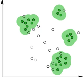
Density-based clustering is based on measuring the data density at a certain region of the data space and then defining clusters as regions that exceed a certain density threshold. The final clusters are obtained by connecting neighboring dense regions. Figure 1 shows an illustrative example in a two-dimensional space. Four groups are recognized as clusters and they are separated by an area where the data density is low.

Fig. 1 Example of density-based clusters [4].

DBSCAN.DBSCAN [12] locates regions of high density that are separated from one another by regions of low density. The approach identifies three different classes of points:

Core points.These points are in the interior of a density-based cluster. A point is a core point if the number of points within a given neighborhood around the point as determined by the distance function and a user- specified distance parameter,

ε, exceeds a certain threshold,MinPts, which is also a user-specified parameter.

Border points.These points are not core points, but fall within the neighborhood of a core point. A border point can fall within the neighborhoods of several core points.

Noise points.A noise point is any point that is neither a core point nor a border point.

The DBSCAN algorithm works as follows: 1. Label all points as core, border, or noise points. 2. Eliminate noise points.

3. Put an edge between all core points that are withinεof each other. 4. Make each group of connected core points into a separate cluster.

5. Assign each border point to one of the clusters of its associated core points. Below we introduce the constraint programming model for this clustering prob-lem.

Constraint Programming Model for Density Based clustering

We reformulate the problem in the context of networks by considering the set of pointsDas nodes and setting an edge between two nodesiand j if the distance between the two points is less than a givenε. Clearly, in this way we have that the

neighbors of a node (point)iare the set of points within a distanceε. Our intended objective is to capture the basic idea that “each node has thesamelabel as all of its neighbors”. Therefore, the problem can be modelled as follows:

maximize(

_∑

j∈L min(1,

_∑

i∈D ki,j)), (29) s.t. ai,j= 1 ifd(i,j)≤ε 0 otherwise ∀i,j∈D (30) ki,j∈ {0,1} ∀i∈D,∀j∈L (31) ri= 1 if∑j∈Dai,j≥minp 0 otherwise ∀i∈D (32)

∑

j∈L ki,j=1 ∀i∈D (33) rh=1∧rp=1∧ah,p=1∧kh,j=1⇒kp,j=1 ∀h∈D,∀r∈D,∀j∈L (34) ri=0⇒ki,j=1 ∀i∈D (35) where j=min({j∈L\ {n+1}| ∃h:ah,i=1∧rh=1∧kh,j=1} ∪ {n+1})

In more detail this model can be described as follows. Boolean variableski,jdenote the color of a point (nodei), by settingki,j=1 if the pointihas the color j. Variables ai,j indicate the presence or absence of an edge between two nodes. Variablesri denote whether nodeiis a core point or not.

Assumed given are: (a) the set of points D, and (b) the ordered set of colors L={1, . . . ,n}. Note that in the set of colors we have the color n+1 that is an additional color used for coloring the noise points. The model imposes that a point has one and only one color, and that all the connected core points must have the same color (Equation 34). Another requirement is that each point that is not a core point takes the same color of the core points that are connected to it. If it does not have any core point around it then this point takes the additional colorn+1 because it is a noise (Equation 35). Such a constraint also captures the special case in which the pointican be connected to more than one core with different colors. In this case,

the model assigns toithe color of the core that in the ordered setC\ {n+1}has a lower rank. Finally, the model is intended to maximize the number of different colors. Notice that a solution where all points have distinct colors does not satisfy Equation 34 because connected points do not have the same color.

This constraint programming formulation makes it easy to extend the standard method with other constraints. In principle, any constraint that requires to merge clusters as identified by DBSCAN can be added to the model above. As an example, we could specify constraints on the minimum cluster size: in this case, clusters will need to be merged in order to obtain a required cluster size; by enforcing a diameter constraint on the resulting clusters, it can be ensured that the resulting clusters are not arbitrary combinations of clusters as identified by traditional DBSCAN.

Moreover, we can also extend the above problem by changing one of the con-straints of the standard formulation. In the following, we will show that by changing a constraint of the DBSCAN formulation we obtain a problem that corresponds to one of the most famous algorithms for discovering communities in network data.

3.2 Label Propagation

When considering graph or network data, a task very similar to clustering is commu-nity discovery, which can be seen as a network variant of standard data clustering. The concept of a “community” in a (web, social, or informational) network is intu-itively understood as a set of individuals that are very similar, or close, to each other, more than to anybody else outside the community [5]. This has often been trans-lated in network terms into finding sets of nodes densely connected to each other and sparsely connected with the rest of the network. An interesting community dis-covery algorithm is the Label Propagation algorithm [17] that detects communities by spreading labels through the edges of the graph and then labeling nodes accord-ing to the majority of the labels attached to their neighbors, iterataccord-ing until a general consensus is reached.

Before introducing a constraint programming model for this algorithm we recall the details of the iterative label propagation algorithm presented in [17].

Iterative Label Propagation (LP).Suppose that a nodevhas neighborsv1,v2, . . . ,vk and that each neighbor carries a label denoting the community that it belongs to. Then, v determines its community based on the labels of its neighbors. [17] as-sumes that each node in the network chooses to join the community to which the maximum number of its neighbors belong to. As the labels propagate, densely con-nected groups of nodes quickly reach a consensus on a unique label. At the end of the propagation process, nodes with the same labels are grouped together as one community. Clearly, a node with an equal maximum number of neighbors in two or more communities will take one of the two labels by a random choice. For clarity, we report here the procedure of the LP algorithm. Note that, in the followingCv(t) denotes the label assigned to the nodevat time (or iteration)t.

1. Initialize the labels at all nodes in the network. For any given nodev,Cv(0) =v. 2. Sett=1.

3. Arrange the nodes in the network in a random order and set it toV.

4. For each vi∈V, in the specific order, letCv_i(t) = f(Cv_i1(t−1), . . . ,Cv_ik(t−1). Function f here returns the label occurring with the highest frequency among neighbors and ties are broken uniformly randomly.

5. If every node has a label that the maximum number of its neighbors has, orthits a maximum number of iterationstmaxthen stop the algorithm. Else, sett=t+1 and go to (3).

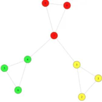
The drawback of this algorithm is the fact thatties are broken uniformly ran-domly. This random behavior can lead to different results for different executions and some of these results cannot be optimal. In Figure 2 we show how given the same network as input of the LP algorithm we obtain four different results.

Fig. 2 The result of four executions of LP Algorithm

In the next section we propose a constraint programming model that solves this problem by providing the optimal solution.

3.2.1 Constraint Programming Model for Label Propagation

Let us now propose a constraint programming model for the community discovering problem based on label propagation. Our aim is to capture the basic idea that “each node takes the label of the majority of its neighborhood”. Therefore, the model is the following: maximize(

_∑

j∈L min(1,

_∑

i∈N ki,j)), (36) s.t. ai,j= 1 if (i,j)∈E 0 otherwise (37) ki,j∈ {0,1} (38)

∑

j∈L ki,j=1 ∀i∈N (39) ni,h=

_∑

∀j:ai,j=1 kj,h ∀i∈N,∀h∈L (40) ki,l=1⇒ni,l=max h∈Lni,h ∀i∈N,∀l∈L (41) Here, variables ai,j indicate the presence or absence of an edge between two nodes. Variableski,j denote the color (label) of a node in the network. Assumed given is (a) the set of nodes N, (b) the set of edges E, and (c) an ordered set of colorsL. A node can be assigned one and only one color. Variablesni,hdenote the number of neighbors of nodeiwith assigned colorh. The model assigns to the node ithe colorhif it is the most popular among its neighbors, as shown in Equation 41. Such a constraint also captures the case of ties. In such a case, nodeiis assigned the color that has the lowest rank in the ordered setL. Finally, the model maximizes the number of different colors in the network, as shown in Equation 36.

This model highlights the similarity between Label Propagation and the Density-based clustering problem, and thanks to the constraint programming formulation we can note that the model for density-based clustering is a variant of the standard label propagation. Indeed, the only difference is due to the fact that the Density-based model requires that “each node has the samelabel of all its neighbors”, and not

themost frequentlabel. Equations 34 and 35 in the DBSCAN model and Equation

41 in the LP model express this difference. By executing our model we obtain the optimal solution depicted in Figure 3, where we consider as input the same network in Figure 2.

4 Conclusions

In this chapter, we have presented how different well-established approaches to partition-based clustering can be modeled and optimized via constraints. In par-ticular, we investigated two main families of partition-based methods, i.e. direct

Fig. 3 The result of the execution of CP-LP model

andindirect. In this perspective, the chapter has presented several examples where

the clustering methods are explicitly modeled by constraints. In this way, it has parted from the more traditionalalgorithmicview on clustering. We discussed dif-ferent optimization criteria and constraints, showed difdif-ferent modeling choices for

directmethods and related theindirectmethods of DBSCAN and label propagation

through a constraint formulation.

References

1. C. C. Aggarwal and C. K. Reddy. Data Clustering: Algorithms and Applications. Chapman & Hall/CRC, 1st edition, 2013.

2. B. Babaki, T. Guns, and S. Nijssen. Constrained clustering using column generation. In H. Si-monis, editor,Lecture Notes in Computer Science, 11th International Conference on Integra-tion of Artificial Intelligence (AI) and OperaIntegra-tions Research (OR) techniques in Constraint Programming (CPAIOR 2014), Cork, Ireland, 19-23 May 2014, pages 438–454. Springer, 2014.

3. S. Basu, I. Davidson, and K. Wagstaff. Constrained Clustering: Advances in Algorithms, Theory, and Applications. Chapman & Hall/CRC, 1 edition, 2008.

4. M. R. Berthold, C. Borgelt, F. Hppner, and F. Klawonn. Guide to Intelligent Data Analysis: How to Intelligently Make Sense of Real Data. Springer Publishing Company, Incorporated, 1st edition, 2010.

5. M. Coscia, F. Giannotti, and D. Pedreschi. A classification for community discovery methods in complex networks.Statistical Analysis and Data Mining, 4(5):512–546, 2011.

6. T. Dao, K. Duong, and C. Vrain. A filtering algorithm for constrained clustering with within-cluster sum of dissimilarities criterion. In2013 IEEE 25th International Conference on Tools with Artificial Intelligence, Herndon, VA, USA, November 4-6, 2013, pages 1060–1067, 2013. 7. T.-B.-H. Dao, K.-C. Duong, and C. Vrain. A declarative framework for constrained clustering.

InECML/PKDD (3), pages 419–434, 2013.

8. T.-B.-H. Dao, K.-C. Duong, and C. Vrain. Constrained clustering by constraint programming.

Artificial Intelligence, pages –, 2015.

9. I. Davidson and S. Ravi. The complexity of non-hierarchical clustering with instance and cluster level constraints.Data Mining and Knowledge Discovery, 14(1):25–61, 2007.

10. I. Davidson and S. S. Ravi. Clustering with constraints: Feasibility issues and the k-means algorithm. InProceedings of the 2005 SIAM International Conference on Data Mining, SDM 2005, Newport Beach, CA, USA, April 21-23, 2005, pages 138–149, 2005.

11. O. du Merle, P. Hansen, B. Jaumard, and N. Mladenovic. An interior point algorithm for minimum sum-of-squares clustering.SIAM J. Sci. Comput., 21(4):1485–1505, Dec. 1999. 12. M. Ester, H.-P. Kriegel, J. Sander, and X. Xu. A density-based algorithm for discovering

clusters in large spatial databases with noise. In E. Simoudis, J. Han, and U. M. Fayyad, editors,KDD, pages 226–231. AAAI Press, 1996.

13. T. F. Gonzalez. Clustering to minimize the maximum intercluster distance. Theor. Comput. Sci., 38:293–306, 1985.

14. P. Hansen and D. Aloise. A survey on exact methods for minimum sum-of-squares clustering.

http://www.math.iit.edu/Buck65files/msscStLouis.pdf, pages 1–2, Jan. 2009.

15. A. K. Jain, M. N. Murty, and P. J. Flynn. Data clustering: A review. ACM Comput. Surv., 31(3):264–323, Sept. 1999.

16. M. Mueller and S. Kramer. Integer linear programming models for constrained clustering. In

Discovery Science - 13th International Conference, DS 2010, Canberra, Australia, October 6-8, 2010. Proceedings, pages 159–173, 2010.

17. U. N. Raghavan, R. Albert, and S. Kumara. Near linear time algorithm to detect community structures in large-scale networks.Physical Review E, 76(2):036106+, 2007.

18. K. Wagstaff and C. Cardie. Clustering with instance-level constraints. InProceedings of the Seventeenth International Conference on Machine Learning (ICML 2000), Stanford Univer-sity, Stanford, CA, USA, June 29 - July 2, 2000, pages 1103–1110, 2000.