Towards Large-Scale Quantum Computation

(1)

arXiv:quant-ph/0506126v1 16 Jun 2005

Towards Large-Scale Quantum

Computation

Austin Greig Fowler

Submitted in total fulfilment of the requirements of the degree of Doctor of Philosophy

March 2005

School of Physics The University of Melbourne

(2)

This thesis deals with a series of quantum computer implementation issues from the Kane 31_{P in} 28_{Si architecture to Shor’s integer factoring} algorithm and beyond. The discussion begins with simulations of the adi-abatic Kane cnot and readout gates, followed by linear nearest neighbor implementations of 5-qubit quantum error correction with and without fast measurement. A linear nearest neighbor circuit implementing Shor’s algo-rithm is presented, then modified to remove the need for exponentially small rotation gates. Finally, a method of constructing optimal approximations of arbitrary single-qubit fault-tolerant gates is described and applied to the specific case of the remaining rotation gates required by Shor’s algorithm.

(3)

Declaration

This is to certify that

1. the thesis comprises only my original work towards the PhD,

2. due acknowledgement has been made in the text to all other material used,

3. the thesis is less than 100,000 words in length, exclusive of tables, maps, bibliographies and appendices.

(4)

This thesis would never have been finished without the help of a number of people. My parents, who have put up with me for more years than I care to mention and have always been there when I needed them. My supervisor, Lloyd Hollenberg, for the freedom he has allowed me and his constant academic and professional support. The DLU, and specifically Maun Suang Boey, for years of assistance above and beyond the call of duty. I am in your debt. I have enjoyed getting to know you as much as working with you. Adam Healy, for his friendship, and, together with Paul Noone, turning my life around. And finally, Natasha, who didn’t help me finish the thesis at all, but showed me I was human.

(5)

List of Figures

1.1 (a) Common single-qubit gates, (b) the cnot gate with solid dot representing the control qubit, (c) the swap gate. . . 6 1.2 (a) Example of a quantum circuit, (b) depth 6 rearrangement

of (a). This circuit implements the encode stage of 5-qubit non-fault-tolerant quantum error correction. . . 7 1.3 Lattice of hypothetical particles used in the construction of the

anyonic model of quantum computation. . . 10 1.4 A conjugate pair of non-Abelian anyons. . . 11 1.5 Performing operations in the anyonic model of quantum

com-putation. . . 11 1.6 Example of the path independence of the phase shift induced

by the Aharonov-Bohm effect. A particle of chargeqexecuting a loop around a perfectly insulated solenoid containing flux Φ acquires a geometric phaseeiqΦ. . . 13 1.7 7-qubit transversal logical cnotgate. . . 17

2.1 Schematic of the Kane architecture. The rightmost two qubits show the notation to be used when discussing thecnot gate. . 25 2.2 Gate profiles and state energies during acnotgate in units of

(10)

2.3 Possible forms of the J(t) profile for step 2 of the adiabatic cnotgate. J(t) is in units ofg_nµ_nB_z= 7.1×10−5meV. . . 31 2.4 The adiabatic measure Θ(t) for each J(t) profile. . . 32 2.5 Probability of error ε during a cnot gate as a function of τ_e

and τn for input state (a)|00i and (b) |01i. The first qubit is

the control. . . 35 2.6 Probability of error ε during a cnot gate as a function of τ_e

and τn for input state (a)|10i and (b) |11i. The first qubit is

the control. . . 36 2.7 The worst case probability of error εduring a cnotgate as a

function ofτe andτn for all input states. . . 37

3.1 Geometry of adiabatic Kane readout. . . 40 3.2 Evolution of the hyperfine and exchange interaction strengths

required to convert nuclear spin information into electron spin information, as shown in Eqs. (3.1–3.4). . . 41 3.3 Probability of error ε during readout state preparation as a

function ofτe andτn for input state (a)|00i and (b) |01i. . . . 43

3.4 Probability of error ε during readout state preparation as a function ofτe andτn for input state|10i. . . 44

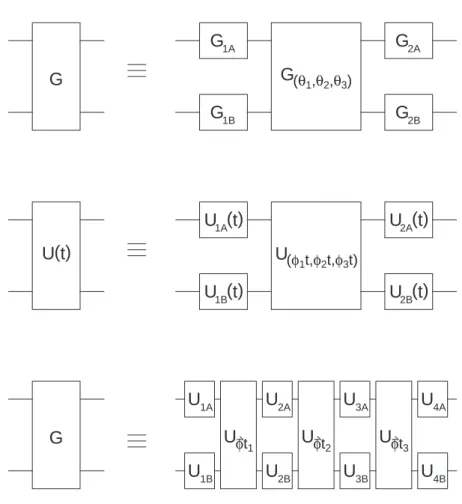
4.1 (a) Circuit equivalent to an arbitrary gate constructed via the canonical decomposition. (b) Similar equivalent circuit which exists for a restricted class of 2-qubit evolution operators. (c) Arbitrary gate expressed as at most three periods evolution of the 2-qubit evolution operator and eight single-qubit gates. . . 47

(11)

List of Figures vii

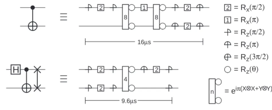
5.1 Decomposition into physical operations of (a) cnot and (b) Hadamard,cnot then swap. Note that the Kane architecture has been used for illustrative purposes. . . 59 5.2 (a) 5-qubit encoding circuit for general architecture, (b)

equiva-lent circuit for linear nearest neighbor architecture with dashed boxes indicating compound gates. cnot gates that must be performed sequentially are numbered. . . 60 5.3 A sequence of physical gates implementing the circuit of Fig. 5.2b.

Note the Kane architecture has been used for illustrative pur-poses. . . 61 5.4 Circuit equivalence used to reduce the number of physical gates

in Fig. 5.3. W =UA2VB1 . . . 61

5.5 A complete encode-wait-decode-measure-correct QEC cycle. . . 61

6.1 Example of a physical model of resetting through relaxation. Given a double potential well with left and right occupancy representing _|0_i and _|1_i respectively, resetting to _|0_i can be achieved by lowering the barrier and applying a bias. . . 68 6.2 Quantum circuit acting on a recently decoded logical qubit to

correct the data qubit based on the value of the ancilla qubits. Hollow dots represent control qubits that must be _|0_i for the attached gate to be applied. . . 69 6.3 Linear nearest neighbor version of Fig. 6.2. . . 70 6.4 5-qubit quantum error correction scheme not requiring fast

(12)

7.1 The complete Shor’s algorithm including classical pre- and post-processing. The first branch is highly likely to fail, resulting in many repetitions of the quantum heart of the algorithm, whereas the second branch is highly likely to succeed. . . 77

7.2 Probability of different measurementsj at the end of quantum period finding with total number of states 22L _{= 256 and (a)}

periodr= 8, (b) period r= 10. . . 80

8.1 (a) Standard quantum Fourier transform circuit. (b) An equiv-alent linear nearest neighbor circuit. . . 87

8.2 (a) Swap gate expressed as a sequence of physical operations via the canonical decomposition. (b) Similarly decomposed com-pound gate consisting of a Hadamard gate, controlled phase rotation, and swap gate. Note that the Kane architecture has been used for illustrative purposes. . . 88

8.3 (a) Quantum Fourier addition. (b) Controlled quantum Fourier addition and its symbolic equivalent circuit. Cont+adenotes the addition ofaifCont= 1. . . 89

(13)

List of Figures ix

8.4 Circuit to compute c = (b+ 2jm2i) modN. The diagonal cir-cuit elements labelled swap represent a series of 2-qubit swap gates. Small gates spaced close together represent compound gates. The qubits x(i) are defined in Eq. 8.2 and essentially store the current partially calculated value of the modular ex-ponentiation that forms the heart of Shor’s algorithm. TheM S (Most Significant) qubit is used to keep track of the sign of the partially calculated modular addition result. The ki qubit is

theith bit ofkin Eq. 8.1. Thekx qubit is set to 1 if and only ifx(i)j =ki = 1. kx±2jm2

i

modN denotes modular addition (subtraction) conditional on kx= 1. . . 91

8.5 Circuit designed to interleave two quantum registers. . . 93

8.6 (a) LNN circuit for the controlled swapping of two qubits _|a_i and_|b_i. The qubits_|a′_iand_|b′_irepresent the potentially swapped states. (b) LNN circuit for the controlled swapping of two quan-tum registers. Note that when chained together, the effective depth of the cswap gate is 4. . . 93

8.7 Circuit designed to modularly multiplyx(i) bym2i

if and only if ki = 1. Note that for simplicity the circuit for L = 4 has

been shown. Note that the bottom L+ 1 qubits are ancilla and as such start and end in the _|φ(0)_i state. The swap gates within the two QFT structures represent compound gates. ki×

(14)

8.8 Circuit implementing the quantum part of Shor’s algorithm. The single-qubit gates interleaved between the modular multi-plications comprise a QFT that has been decomposed by using measurement gates to remove the need for controlled quantum phase rotations. Note that without these single-qubit gates the remaining circuit is simply modular exponentiation. . . 97

9.1 Circuit for a 4-qubit (a) quantum Fourier transform and (b) approximate quantum Fourier transform with dmax= 1. . . 100

9.2 Decomposition of a controlled phase gate into single-qubit ro-tations and acnotgate. . . 103

9.3 Probability sof obtaining useful output from quantum period finding as a function of period r for different integer lengths L and rotation gate restrictions π/2dmax_{. The effect of using} inaccurate controlled rotation gates (σ=π/32) is shown in (e). 104

9.4 Dependence of the probability of useful output from the quan-tum part of Shor’s algorithm on the length L of the integer being factored for different levels of restriction of controlled ro-tation gates of angleπ/2dmax_{. The parameter}_L

0 characterizes lines of best fit of the forms_∝2−L/L0_{. . . 105}

10.1 Non-fault-tolerant 7-qubit Steane code encoding circuits taking an arbitrary stateα_|0_i+β_|1_i and producingα_|0Li+β|1Li. (a)

Depth 4 circuit for an architecture able to interact arbitrary pairs of qubits. (b) Depth 5 circuit for a linear nearest neighbor architecture. . . 114

(15)

List of Figures xi

10.2 Circuits fault-tolerantly applying common single-qubit gates to Steane code logical qubits. Gates in brackets are optional as they implement stabilizers. . . 117 10.3 High-level representation of the circuit implementing the T

-gate on a Steane code logical qubit. Input α_|0Li+β|1Li is

transformed into α_|0Li+βeiπ/4|1Li. . . 117

10.4 Circuit measuring whether_|Ψ_i is in the +1 or₋1 eigenstate of A. . . 118 10.5 (a) Simple circuit fault-tolerantly preparing a cat state. (b)

Circuit undoing the preparation of a cat state. . . 119 10.6 Typical, but unnecessarily complicated circuit fault-tolerantly

preparing a cat state. . . 120 10.7 Symbolic representation of transversal controlled operations. . . 121 10.8 Circuit fault-tolerantly projecting _|Ψ_i onto the _±1 eigenstates

ofXIXIXIX, then converting₋1 eigenstate’s into +1 eigenstates. The third measurement structure can be omitted if M1=M2. . 121 10.9 Circuit taking arbitrary input and producing_|0Li by repeated

stabilizer measurement. . . 122 10.10 Circuit taking arbitrary input and producing_|0Li via physical

resetting and just three stabilizer measurements. . . 122 10.11 Complete circuit implementing the T-gate on a Steane code

logical qubit. . . 124 10.12 Optimal fault-tolerant approximationsUlof phase rotation gates

R₂d, forR₈ to R₁₂₈. . . 126

10.13 Non-fault-tolerant circuit exactly implementing R128 by first decoding the logical qubit and re-encoding after application of R128. . . 128

(16)

10.14 Schematic of a minimum complexity, sufficiently accurate fault-tolerant approximation ofR128 given in full by Eq. (10.26). . . 128 10.15 Circuit fault-tolerantly correcting an arbitrary single error within

the logical qubit. The qubit acted on by the correctZ/Xboxes is described by Table 10.2. . . 129 10.16 Approximate probability of more than one error in the output

logical qubit versus probability per qubit per time step of dis-crete error for different circuits implementing aR128 phase ro-tation gate. (a) NFT: non-fault-tolerant circuit from Fig. 10.13, (b) FT I: fault-tolerant circuit from Fig. 10.14, (c) FT II: as above but with Fig. 10.15 error correction after every second T-gate, (d) FT III: as above but with error correction after every T-gate. Note that all fault-tolerant results are for the 7-qubit Steane code without concatenation. . . 130 10.17 Average accuracy of optimal fault-tolerant gate sequence

(17)

List of Tables

5.1 Action required to correct the data qubit Ψ′ _{vs measured value} of ancilla qubits. Note that the X-operations simply reset the ancilla. . . 62 5.2 Probability per time step ǫstep of the logical qubit being

de-stroyed when using 5-qubit QEC vs physical probability p per qubit per time step of a discrete error. . . 64 5.3 Probability per time step ǫstep of the logical qubit being

de-stroyed when using 5-qubit QEC vs standard deviation σ of continuous errors. . . 65 6.1 Second column shows the action required to correct the data

qubit given a certain ancilla value immediately after decoding. Third column shows the action required to correct the data qubit given a certain ancilla value after the application of the first half of Fig. 6.2. . . 70 6.2 Probability per time step ǫstep of the logical qubit being

de-stroyed when using no measurement 5-qubit QEC vs physical probability pper qubit per time step of a discrete error. . . 71 6.3 Probability per time step ǫstep of the logical qubit being

de-stroyed when using no measurement 5-qubit QEC vs standard deviationσ of continuous errors. . . 71

(18)

7.1 Required number of qubits and circuit depth of different im-plementations of the quantum part of Shor’s algorithm. Where possible, figures are accurate to leading order inL. . . 76

10.1 Best case complexity of the T-gate. . . 124 10.2 Qubit to correct given certain sequence of eigenvalue

(19)

1. Introduction

This chapter begins with a brief review of the quantum computing field with a bias towards the specific topics developed in later chapters. The main purpose of the review is to introduce the concepts and language required to overview the aims and content of this thesis (Section 1.4). The reader familiar with quantum computing can go directly to Section 1.4. Familiarity with quantum mechanics is assumed.

In Section 1.1 we provide justification and motivation for the study of quantum computing. Section 1.2 reviews the various models of quantum computation, namely the circuit model, adiabatic quantum computation, cluster states, topological quantum computation, and geometric quantum computation. The theoretical work demonstrating that arbitrarily large quantum computations can be performed arbitrarily reliably is gathered in Section 1.3. Section 1.4 then overviews the thesis.

1.1 Why quantum compute?

The incredible exponential growth in the number of transistors used in con-ventional computers, popularly described as Moore’s Law, is expected to continue until at least the end of this decade [1]. This growth is achieved through miniaturization. Smaller transistors consume less power, can be packed more densely, and switch faster. However, in some areas,

(20)

particu-larly the silicon dioxide insulating layer within each transistor, atomic scales are already being approached [2]. This fundamental barrier is one of many factors fuelling research into radical new computing technologies.

Furthermore, certain problems simply cannot be solved efficiently on conventional computers irrespective of their inexorable technological and computational progress. One such problem is the simulation of quantum systems. The amount of classical data required to describe a quantum sys-tem grows exponentially with the syssys-tem size. The data storage problem alone precludes the existence of an efficient method of simulation on a con-ventional computer.

The first hint of a way around this impasse was provided by Feynman in 1982 [3] when he suggested using quantum mechanical components to store and manipulate the data describing a quantum system. The number of quantum mechanical components required would be directly proportional to the size of the quantum system. This idea was built on by Deutsch in 1985 [4] to form a model of computation called a quantum Turing machine — the quantum mechanical equivalent of the universal Turing machine [5] which previously was thought to be the most powerful and only model of computation.

That the laws of physics in principle permit the construction of quan-tum computers exponentially more powerful than their classical relatives is hugely significant. Despite this, it was not until the publication of Shor’s quantum integer factoring algorithm [6] that research into quantum comput-ing began to attract serious attention. The difficulty of classically factorcomput-ing integers forms the basis of the popular RSA encryption protocol [7]. RSA is used to establish secure connections over the Internet, enabling the trans-mission of sensitive data such as passwords, credit card details, and online

(21)

1.2. Models of quantum computing 3

banking sessions. RSA also forms the heart of the popular secure messaging utility PGP (Pretty Good Privacy) [8]. Rightly or wrongly, the prospect of rendering much of modern classical communication insecure has arguably driven the race to build a quantum computer.

More recently, quantum algorithm offering an exponential speed up over their classical equivalents have been devised for problems within group the-ory [9], knot thethe-ory [10], eigenvalue calculation [11], image processing [12], basis transformations [13], and numerical integrals [14]. Other promising quantum algorithms exist [15, 16], but have not been thoroughly analyzed. On the commercial front, the communication of quantum data has been shown to enable unconditionally secure communication in principle [17] re-sulting in the creation of companies offering real products [18, 19] that have already found application in the information technology sector [20]. Despite this, it remains to be seen whether human ingenuity is sufficient to make large-scale quantum computing a reality.

1.2 Models of quantum computing

Classical computers have a single well defined computational model — the direct manipulation of bits via Boolean logic. The field of quantum compu-tation is too young to have settled on a single model. This section attempts to make a brief yet complete review of the current status of the various quantum computation models currently under investigation. We neglect quantum Turing machines [4] as they are a purely abstract rather than a physically realisably computation model. We also neglect quantum neural networks [21, 22] due to their use of nonlinear gates, and both Type II quantum computers [23] and quantum cellular automata [24] due to their essentially classical nature.

(22)

1.2.1 The circuit model

The most widely used model of quantum computation is called the circuit model. Instead of the traditional bits of conventional computing which can take the values 0 or 1, the circuit model is based on qubits which are quantum systems with two states denoted by _|0_i and _|1_i. The power of quantum computing lies in the fact that qubits can be placed in superpositionsα_|0_i+ β_|1_i, and entangled with one another, eg. (_|00_i+_|11_i)/√2. Manipulation of qubits is performed via quantum gates. Ann-qubit gate is a 2n_×2nunitary matrix. The most general single-qubit gate can be written in the form

U =    ei(α+β)/2cosθ ei(α−β)/2sinθ −ei(−α+β)/2sinθ e−i(α+β)/2cosθ   . (1.1)

Common single-qubit gates are

H = √1 2    1 1 1 ₋1   , X=    0 1 1 0   , Z =    1 0 0 ₋1   , S=    1 0 0 i   , S †₌    1 0 0 ₋i   , T =    1 0 0 eiπ/4   . (1.2)

For example, the result of applying anX-gate toα_|0_i+β_|1_i is

   0 1 1 0       α β   =    β α   . (1.3)

The X-gate will sometimes be referred to as a not gate or inverter. Its action will sometimes be referred to as a bit-flip or inversion, and that of the Z-gate as a phase-flip. TheH-gate was derived from the Walsh-Hadamard transform [25, 26] and first named as the Hadamard gate in [27].

(23)

Given the ability to implement arbitrary single qubit gates and almost any multiple qubit gate, arbitrary quantum computations can be performed [28, 29]. The column vector form of an arbitrary 2-qubit state_|Ψ_i=α_|00_i+ β_|01_i+γ_|10_i+δ_|11_i is           α β γ δ           . (1.4)

Note the ordering of the computational basis states. For convenience, such states will occasionally be denoted by _|q1q0i withq1 (q0) referred to as the first (last) or left (right) qubit regardless of the actual physical arrangement. The most common 2-qubit gate is the controlled-not (cnot)

          1 0 0 0 0 1 0 0 0 0 0 1 0 0 1 0           , (1.5)

which given an arbitrary 2-qubit state _|q1q0i, inverts the target qubit q0 if the control qubitq1 is 1. Note that acnotwith target qubitq1 and control qubitq0 would have the form

          1 0 0 0 0 0 0 1 0 0 1 0 0 1 0 0           . (1.6)

(24)

X Z S H T S (a) (b) (c)

Fig. 1.1: (a) Common single-qubit gates, (b) thecnot gate with solid dot repre-senting the control qubit, (c) the swap gate.

The swap gate

          1 0 0 0 0 0 1 0 0 1 0 0 0 0 0 1           (1.7)

swaps the states of q1 and q0. Additional 2-qubit gates will be defined as required.

By representing qubits as horizontal lines, a time sequence of quantum gates can conveniently be represented by notation that looks like a conven-tional circuit. Symbols equivalent to the gates described above are shown in Fig. 1.1. An example of a complete circuit is shown in Fig. 1.2a. Note that the horizontal lines represent time flowing from left to right, not wires. We define the depth of a quantum circuit to be the number of layers of 2-qubit gates required to implement it. Note that multiple single-qubit gates and 2-qubit gates applied to the same two qubits can be combined into a single 2-qubit gate. For example, Fig. 1.2b is a depth 6 rearrangement of Fig. 1.2a. These circuits are discussed in more detail in Chapter 5.

The basis _{|0_i,_|1_i} is referred to as the computational basis. The sim-plest representation of ann-qubit state is

|Ψ_i= √1 2n 2n₋₁ X k=1 |k_i, (1.8)

(25)

1.2. Models of quantum computing 7 (a) Ψ (b) H H H 0 H H H 1 2 3 4 5 6 1 2 3 4 5 6 0 0 0 Ψ 0 0 0 0 ΨL ΨL

Fig. 1.2: (a) Example of a quantum circuit, (b) depth 6 rearrangement of (a). This circuit implements the encode stage of 5-qubit non-fault-tolerant quantum error correction.

have undergone investigation by many authors and are well reviewed in [30].

One natural extension of the qubit circuit model is to used-level quantum systems (qudits). The simplest representation of ann-qudit state is

|Ψ_i= √1 dn dn₋₁ X k=1 |k_i, (1.9)

where k is expressed in base d. The properties of qudit entanglement [31], qudit teleportation [32], qudit error correction [33, 34], qudit cryptography [35, 36], and qudit algorithms [37, 38] are broadly similar to the correspond-ing properties of qubits, and will not be discussed further here.

A third variant of the circuit model exists based on continuous quan-tum variables such as the position and momenquan-tum eigenstates of photons. Considerable experimental work on the entanglement of continuous quan-tum variables has been performed and is reviewed in Ref. [39]. In particular, the problem of continuous quantum variable teleportation [40] has received a great deal of attention. Furthermore, methods have been devised to perform continuous variable error correction [41], cryptography [42], and continuous variable versions of a number of algorithms [43, 44, 45, 46].

(26)

1.2.2 Adiabatic quantum computation

In the adiabatic model of quantum computation [47], a Hamiltonian Hf

is found such that its ground state is the solution of the problem under consideration. This final Hamiltonian Hf must also be continuously

de-formable (for example, by varying the strength of a magnetic field) to some initial Hamiltonian Hi with a ground state that is easy to prepare. After

initializing the computer in the ground state ofHi, Hi is adiabatically (i.e.

sufficiently slowly to leave the system in the ground state) deformed intoHf

yielding the ground state of Hf. The major difficulty is determining how

slowly the deformation must occur to be adiabatic. The adiabatic model can be applied to systems of qubits, qudits, and continuous quantum vari-ables, and is equivalent to the circuit model in the sense that any adiabatic algorithm can be converted into a quantum circuit with at most polyno-mial overhead [48, 49]. The principal advantage of the adiabatic model is an alternative way of thinking about quantum computation that has led to numerous new algorithms tackling problems in graph theory [50], combina-torics [47, 51], condensed matter and nuclear physics [52], and set theory [53].

1.2.3 Cluster states

Given a multi-dimensional lattice of qubits each initialized to (_|0_i+_|1_i)/√2 with identical tunable nearest neighbor interactions of form

Hij(t) = ¯hg(t)(1 +σz(i))(1 +σ(zj))/4, (1.10)

a cluster state [54] can be created by evolving the system for a time such that

R

(27)

property that arbitrary quantum computations can be performed purely via single-qubit measurements along arbitrary axes [55, 56]. A small amount of classical computation is required between measurements. Cluster states can also be defined over qudits [57], and are special cases of the more general class of graph states [58]. Methods have been devised to perform quantum communication [59], error correction [60] and fault-tolerant computation [61] within the cluster state model. Entanglement purification can be used to increase the reliability of cluster state generation [62]. Unlike the adiabatic model however, the cluster state model is yet to lead to any genuinely new algorithms. Given the equivalence of the cluster state model to the circuit model [63], the primary utility of the cluster state model appears to be simpler physical implementation in certain systems such as linear optics [64, 65], and possibly special cases of NV-centers in diamond, quantum dots, and ion traps [66].

1.2.4 Topological quantum computation

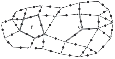
The primary difficulty in building a quantum computer is controlling data degradation through interaction with the environment, generally called deco-herence. Interaction with the environment can in principle be eliminated by using a topological model of computation. Topological quantum computa-tion was proposed by Kitaev in 1997 [67], and developed further in Ref. [68]. An alternative proposal was given by Freedman in Ref. [69]. Kitaev consid-ered an oriented 2-dimensional lattice of hypothetical particles with many body interactions as shown in Fig. 1.3. The hypothetical particles on each lattice link are related to the 60 permutations of five distinguishable objects P5. Certain types of excitations of the lattice are also related to the group P5, and exist on lattice sites which correspond to a vertex and face pair

(28)

f

v

Fig. 1.3: Lattice of hypothetical particles used in the construction of the anyonic model of quantum computation.

as shown in Fig. 1.4. These excitations are called non-Abelian anyons. Of particular interest are pairs of excitations_|g, g−1_i_{. Non-Abelian anyon pairs} have the remarkable property that simply moving them through one an-other effects computation. Given two pairs_|g, g−1_i,_|h, h−1_i, moving_|g, g−1_i through _|h, h−1_i as shown in Fig. 1.5 creates the state _|hgh−1, hg−1h−1_i.

Let _|0_i = _|g, g−1_i and _|1_i = _|h, h−1_i. Find x such that h = xgx−1. A quantum inverter can be constructed simply by moving states _|0_i,_|1_i through the ancilla pair_|x, x−1_i. More complicated operations can be per-formed simply in a similar manner, using more ancilla pairs and pull through operations.

At sufficiently low temperature, the only way data can be corrupted in a topological quantum computer is via the spontaneous interaction of two anyons — an event that occurs with probability O(e−αl_{), where} _l _{is the}

minimum separation of any pair of anyons. This probability can be made arbitrarily small simply by keeping the anyons well separated. While this is a desirable property, clearly a computational model based on hypothetical

(29)

g

-1

Fig. 1.4: A conjugate pair of non-Abelian anyons.

g-1 _h-1

g h

h-1

h hgh-1

hg-1_h-1

(30)

particles that do not exist in nature cannot be implemented.

Recently, significant progress has been made on the topological quantum computation model. General schemes using anyons based on arbitrary non-solvable groups [70], and smaller, non-solvable, non-nilpotent groups [71] have been devised. A less robust but simpler scheme based on Abelian anyons has been proposed [72] and designs for possible experimental realizations are emerging [73, 74]. Experimental proposals based on non-Abelian anyons have also been constructed [75, 76].

1.2.5 Geometric quantum computation

The basic idea of geometric quantum computation is illustrated by the Aharonov-Bohm effect [77] in which a particle of charge q executing a loop around a perfectly insulated solenoid containing flux Φ acquires a geomet-ric phaseeiqΦ [78]. As shown in Fig. 1.6, the phase acquired is insensitive to the exact path taken. This phase shift can be used to build quantum gates [79, 80]. At the moment, there are conflicting numerical and analytic calculations both supporting and attacking the fundamental robustness of geometric quantum computation [81].

1.3 Quantum computation is possible in principle

For the remainder of the thesis we will focus on the qubit circuit model. Physical realizations of this model of computation have been proposed in the context of liquid NMR [82], ion traps [83] including optically [84, 85] and physically [86, 87] coupled microtraps, linear optics [88], Josephson junctions utilizing both charge [89, 90] and flux [91] degrees of freedom, quantum dots [92], 31P in 28Si architectures utilizing indirectly exchange coupled donor nuclear spins [93], exchange coupled electron spins [94, 95],

(31)

1.3. Quantum computation is possible in principle 13

eiqΦ

Φ

eiqΦ

Fig. 1.6: Example of the path independence of the phase shift induced by the Aharonov-Bohm effect. A particle of chargeq executing a loop around a perfectly insulated solenoid containing flux Φ acquires a geometric phase

eiqΦ

.

both spins [96, 97], magnetic dipolar coupled electron spins [98] and qubits encoded in the charge distribution of a single electron on two donors [99], deep donors in silicon [100], acceptors in silicon [101], solid-state ensemble NMR utilizing lines of 29Si in 28Si [102], electrons floating on liquid helium [103], cavity QED [104, 105], optical lattices [106, 107] and the quantum Hall effect [108]. At the present time, the ion trap approach is the closest to realizing the five basic requirements of scalable quantum computation [109]. The mere existence of quantum computer proposals and quantum algo-rithms is not sufficient to say that quantum computation is possible in prin-ciple. Firstly, almost all quantum algorithms that provide an exponential speed up over the best-known equivalent classical algorithms make use of the quantum Fourier transform which in turn uses exponentially small rotations. For example, in the case of Shor’s algorithm, to factor an L-bit number, in principle single-qubit rotations of magnitude 2π/22L are required. Clearly

(32)

this is impossible for largeL.

Coppersmith resolved this issue by showing that most of the small ro-tations in the quantum Fourier transform could simply be ignored without significantly affecting the output of the circuit. For the specific case of Shor’s algorithm, as described in Chapter 9, we took this work further to show that rotations of magnitudeπ/128 implemented with accuracy_±π/512 were sufficient to factor integers thousands of bits long.

More seriously, quantum systems are inherently fragile. The gamut of relaxation processes, environmental couplings, and even systematic errors in-duced by architectural imperfections are typically grouped under the head-ing of decoherence. Ignorhead-ing leakage errors in which a qubit is destroyed or placed in a state other than those selected for computation [110], Shor made the surprising discovery that all types of decoherence could be cor-rected simply by correcting unwanted bit-flips (X), phase-flips (Z) and both simultaneously (XZ) [111]. Shor’s scheme required each qubit of data to be encoded across nine physical qubits. This was the first quantum error correction code (QECC).

Later work by Laflamme gave rise to a 5-qubit QECC [112] — the small-est code that can correct an arbitrary error to one of its qubits [30]. Steane’s 7-qubit code [113], which also only guarantees to correct an arbitrary error to one of its qubits, is, however, more convenient for the purposes of quan-tum computation. Steane’s code is part of the large class of CSS codes (Calderbank, Shor, Steane) [114], which is in turn part of the very large class of stabilizer codes [115]. Only a few examples such as permutationally invariant codes [116] exists outside the class of stabilizer codes.

To illustrate the utility of the stabilizer formalism, consider a 5-qubit QECC [117] in which we create logical _|0_i and _|1_i states corresponding to

(33)

1.3. Quantum computation is possible in principle 15 the superpositions |0Li = |00000i+|10010i+|01001i+|10100i +_|01010_{i − |}11011_{i − |}00110_{i − |}11000_i −|11101_{i − |}00011_{i − |}11110_{i − |}01111_i −|10001_{i − |}01100_{i − |}10111_i+_|00101_i, (1.11) |1Li = |11111i+|01101i+|10110i+|01011i +_|10101_{i − |}00100_{i − |}11001_{i − |}00111_i −|00010_{i − |}11100_{i − |}00001_{i − |}10000_i −|01110_{i − |}10011_{i − |}01000_i+_|11010_i. (1.12)

These superstitions redundantly encode data in such a way that an arbitrary error to any one qubit can be corrected. They are, however, difficult to work with directly. In the stabilizer formalism,_|0Liand|1Liare instead described

as simultaneous +1 eigenstates of

M1 = X⊗Z⊗Z⊗X⊗I (1.13)

M2 = I⊗X⊗Z⊗Z⊗X (1.14)

M3 = X⊗I⊗X⊗Z⊗Z (1.15)

M4 = Z_⊗X_⊗I _⊗X_⊗Z (1.16)

These operators are called stabilizers. Let S denote the set of stabilizers (which is the group generated by M1–M4). Any valid logical state must satisfy M_|ΨLi = |ΨLi for all M ∈ S. This observation allows us to

de-termine which quantum gates can be applied directly to the logical states. Specifically, if we wish to applyU to our logical state to obtainU_|ΨLi, then

(34)

since U M U†U_|Ψ_i must be a logical state, U M U† must be a stabilizer. If we restrict our attention to gatesU that are products of single-qubit gates, only two single logical qubit gates

XL = X⊗X⊗X⊗X⊗X (1.17)

ZL = Z⊗Z⊗Z⊗Z⊗Z (1.18)

can be applied directly to data encoded using this version of 5-qubit QEC. Note that by restricting our attention to products of single-qubit gates, any error present in one of the qubits of the code before a logical gate operation cannot be copied to other qubits. Any circuit with the property that a single error can cause that most one error in the output is called fault-tolerant.

So far, we have not explained how errors are corrected using a QECC. Given a potentially erroneous state _|Ψ′_i, one way of locating any errors is to check whether_|Ψ′_iis still a +1 eigenstate of each of the stabilizers. Any errors so located can then be manually corrected. This method is described in some detail in Chapter 10.

We now have basic single logical qubit gates and error correction. To achieve universal quantum computation we need to be able to couple logical qubits and perform arbitrary single logical qubits gates [28, 29]. Unfortu-nately, the 5-qubit QECC does not readily permit multiple logical qubits to be coupled, though a complicated three logical qubit gate does exist [118]. For universal quantum computation, the 7-qubit Steane code, or indeed any of the CSS codes, is more appropriate as they permit a simple transversal implementation of logical cnot as shown in Fig. 1.7. The 7-qubit Steane code also permits similar transversal single-qubit gates H, X, Z, S and S† (see Fig. 10.2). These are, however, insufficient to construct arbitrary

(35)

7

Fig. 1.7: 7-qubit transversal logicalcnotgate.

single-qubit rotations of the form

   cos(θ/2)ei(α+β)/2 sin(θ/2)ei(α−β)/2 −sin(θ/2)ei(−α+β)/2 cos(θ/2)ei(−α−β)/2   . (1.19)

An additional gate such as the T-gate is required to construct arbitrary single-qubit gates. The simplest fault-tolerant implementation of theT-gate we have been able to devise still requires an additional 12 ancilla qubits, and at least 93 gates, 45 resets and 17 measurements arranged on a circuit of depth at least 92 and is described in detail in Chapter 10. By virtue of the fact that the operation HT corresponds to the rotation of a qubit by an angle that is an irrational number, and the fact that repeated rotation by an irrational number enables arbitrarily close approximation of a rotation of any angle, the pair of single-qubit gatesH,T is sufficient to approximate an arbitrary single-qubit rotation arbitrarily accurately. In practice, it is

(36)

better to use the 23 unique combinations ofH,X,Z,S and S†in addition to the T-gate since, for example, the logical X-gate is vastly simpler to implement thanHT T T T H. The existence of efficient sequences of gates to approximate arbitrary unitary rotations in general, and single-qubit gates in particular, is guaranteed by the Solovay-Kitaev theorem [119, 120, 30, 121]. The exact length of such sequences required to achieve a given accuracy is discussed in Chapter 10.

We now have enough machinery to consider arbitrarily large, arbitrarily reliable quantum computation. Suppose every qubit in our computer has probability p of suffering an error per unit time, where unit time refers to the amount of time required to implement the slowest fundamental gate (not logical gate). Consider a circuit consisting of the most complicated fault-tolerant logic gate, the T-gate, followed by quantum error correction. By virtue of being fault-tolerant, this circuit can only fail to produce useful output if at least two errors occur. For some constant c, and sufficiently low error ratep, the probability of failure of the structure is thuscp2. Since we have chosen the most complicated gate, every other fault-tolerant gate followed by error correction, including the identityI (do nothing) gate, has probability of failure at most cp2_.

Consider an arbitrary quantum circuit expressed in terms of the funda-mental gates cnot,I, H,X, Z, S,S†, their products, andT (no QEC at this stage). In the worst-case, if an error anywhere causes the circuit to fail, the probability of success of such a circuit is (1₋p)qt_where_q _{is the number}

of qubits and t the number of time steps. By replacing each gate with an error corrected fault-tolerant structure, this can be reduced to (1₋cp2)qt. Note that the new circuit is still expressed entirely in terms of the allowed gates and measurement. We can therefore repeat the process and replace

(37)

these gates in turn with error corrected fault-tolerant structures giving an overall reliability of (1₋c3p4)qt. If we repeat this ktimes we find that the overall circuit reliability is

1₋(cp) 2k

c

!qt

. (1.20)

Clearly, provided the error rate per time step is less thanpth= 1/c and we

have sufficient resources, an arbitrarily large quantum computation can be performed arbitrarily reliably. This is the threshold theorem of quantum computation [122]. Note that the greater the amount p < pth, the fewer

levels of error correction that are required. Despite the lack of a definitive reference,pth is frequently assumed to be 10−4.

Substantial customization and optimization of the threshold theorem has occurred over the years. As described, the threshold theorem requires the ability to interact arbitrarily distant pairs of qubits in parallel, fast measure-ment gates, and fast and reliable classical computation. A detailed study of the impact of noisy long-range communication has been performed yielding threshold error rates _∼10−4 for a variety of assumptions [123]. Modifica-tions removing the need for measurement and classical processing but still requiring error-free long-range interactions have been devised at the cost of greatly increased resources [124], though subsequent work has substantially reduce the complexity of the required quantum circuitry with a threshold pth= 2.4×10−6obtained under the additional assumption that the quantum

computer consists of a single line qubits with nearest neighbor interactions only [125].

By using a much simplified error correction scheme devised by Steane [126] that works on any CSS code, and using larger QECCs and less

(38)

concate-nation, encouragingly high thresholds_∼10−3 [127] and even 9_×10−3 [128] have been calculated, although in the latter case only under the assumption that errors occur after gates, not to idle qubits, and in both cases long-range interactions must be available.

An alternative approach is to perform computation by interacting data with specially prepared ancilla states [129, 130], a method called postselected quantum computing. While the resources required to prepare sufficiently reliable ancilla states are prohibitive, in principle this approach permits arbitrarily large computations to be performed provided p < pth = 0.03

[131].

1.4 Overview

The primary goal of this thesis is to relax the theoretical resource require-ments required for large-scale quantum computation. Much of our work is motivated by the Kane 31_{P in} 28_{Si architecture in which fast and reliable} measurement and classical processing is difficult to achieve, and qubits may be limited to a single line with nearest neighbor interactions only.

In Chapters 2–3, the viability of the adiabatic Kanecnotgate and read-out operation are assessed. Chapter 4 reviews a technique of constructing efficient 2-qubit gates. A greatly simplified non-fault-tolerant linear nearest neighbor implementation of 5-qubit quantum error correction is presented in Chapter 5, and further modified to remove the need for measurement and classical processing in Chapter 6. Chapter 7 provides a detailed review of Shor’s algorithm, followed by a linear nearest neighbor circuit implementa-tion in Chapter 8. Chapter 9 focuses on removing the need for exponen-tially small rotations in circuit implementations of Shor’s algorithm. Finally, Chapter 10 presents a method of constructing arbitrary single-qubit

(39)

fault-1.4. Overview 21

tolerant gates, and applies this to the specific case of the remaining rotation gates required by Shor’s algorithm. Chapter 11 contains concluding remarks and summarizes the results of the thesis. Chapters 2, 3, 5, 8 and 9 have been published in [132, 133, 134, 135, 136] respectively.

(40)

(41)

2. The adiabatic Kane

cnot

gate

The spins of the31P nucleus and donor electron in bulk28Si have extremely long coherence times [137, 138]. Consequently, a number of quantum com-puter proposals have been based on this system [93, 97, 98, 95]. In this chapter and Chapter 3, we focus on Kane’s 1998 proposal [93] which calls for a line of single31_{P atoms spaced approximately 20nm apart [139, 140].} The spin of each phosphorus nucleus is used as a qubit and the donor elec-tron used to couple to neighboring qubits. Neglecting readout mechanisms for the moment, each qubit requires at least two electrodes to achieve single-and 2-qubit gates. The extent to which the presence single-and operation of these electrodes will reduce the system’s coherence times is unknown. We there-fore study the error rate of the Kanecnotgate as a function of the coherence times to determine their approximate minimum acceptable values. We find that the coherence times required to achieve acnot error rate of 10−4 are a factor of 6 less than those already observed experimentally.

The chapter is organized as follows. In Section 2.1, the Kane architec-ture is briefly described followed by the method of performing a cnot in Section 2.2. In Section 2.3, the technique we used to model finite coherence times is presented along with contour plots of thecnoterror rate as a func-tion of the coherence times. In Secfunc-tion 2.4, we discuss the implicafunc-tions of our results.

(42)

2.1 The Kane architecture

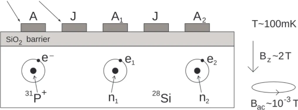
Ignoring readout mechanisms, which we discuss in Chapter 3, the basic lay-out of the adiabatic Kane phosphorus in silicon solid-state quantum com-puter [93, 96] is shown in Fig. 2.1. The phosphorous donor electrons are used primarily to mediate interactions between neighboring nuclear spin qubits. As such, the donor electrons are polarized to remove their spin degree of freedom. This can be achieved by maintaining a steadyBz = 2T at around

T = 100mK [141]. Techniques for relaxing the high field and low tempera-ture requirements such as spin refrigeration are under investigation [96].

In addition to the potential to build on the vast expertise acquired dur-ing the last 50 years of silicon integrated circuit development, the primary attraction to the Kane architecture, and31P in28Si architectures in general, is their extraordinarily long spin coherence times [137, 138]. Four quantities are of interest — the relaxation (T1) and dephasing (T2) times of both the donor electron and nucleus. Both times only have meaning when the system is in a steady magnetic field. Assuming the field is parallel with the z-axis, the relaxation time refers to the time taken for 1/eof the spins in the sample to spontaneously flip whereas the dephasing time refers to the time taken for thex and y components of a single spin to decay by a factor of 1/e. Exist-ing experiments cannot measureT2 directly, but instead a third quantityT2∗ which is the time taken for thexand y components of an ensemble of spins to decay by a factor of 1/e. Since T₂∗ _≤T2 [142], we can use experimental valuesT∗

2 as a lower bound forT2.

In natural silicon containing 4.7% 29_{Si, relaxation times} _T

1 in excess 1 hour have been observed for the donor electron atT = 1.25K andB _∼0.3T [137]. The nuclear relaxation time has been estimated at over 80 hours in similar conditions [143]. These times are so long that we will ignore

(43)

relax-2.1. The Kane architecture 25

ation in our simulations of gate reliability. The donor electron dephasing timeT₂∗ in enriched28Si containing less than 50ppm29Si, at 7K and donor concentration 0.8_×1015 has been measured to be 14ms [138]. Extrapo-lation to a single donor suggests T2 = 60ms at 7K. An even longer T2 is expected at lower temperatures. At the time of writing, to the authors’ knowledge, no experimental data relating to the nuclear dephasing time has been obtained. However, considering the much greater isolation from the environment of the nuclear spin, this time is expected to be much larger than the electron dephasing time.

A

J

A

J

A

Si

28

e

_

P

31 + barrier B_ac~10-3T z B ~2T T~100mK SiO₂ Electrodes

e

1

e

2

n

1

n

2 1 2

Fig. 2.1: Schematic of the Kane architecture. The rightmost two qubits show the notation to be used when discussing the cnotgate.

Control of the nuclear spin qubits is achieved via electrodes above and between each phosphorus atom and global transverse oscillating fields of magnitude_∼10−3_{T. To selectively manipulate a single qubit, the}_A_-electrode above it is biased. A positive/negative bias draws/drives the donor electron away from the nucleus, in both cases reducing the magnitude of the hyperfine interaction. This in turn reduces the energy difference between nuclear spin up (_|0_i) and down (_|1_i) allowing this transition to be brought into resonance with a globally applied oscillating magnetic field. Depending on the timing

(44)

of theA-electrode bias, an arbitrary rotation about an axis in thex-yplane can be implemented [144]. By utilizing up to three such rotations, a qubit can be rotated into an arbitrary superpositionα_|0_i+β_|1_i.

Biasing an A-electrode above a particular donor will also effect neigh-boring and more distant donors. It is likely that compensatory biasing of nearby electrodes will be required to ensure non-targeted qubits remain off resonant. Subject to this restriction, there is no limit to the number of simultaneous single-qubit rotations that can be implemented throughout a Kane quantum computer.

Interactions between neighboring qubits are governed by theJ-electrodes. A positive bias encourages greater overlap of the donor electron wave func-tions leading to indirect coupling of their associated nuclei. In analogy to the single-qubit case, this allows multiple 2-qubit gates to be performed se-lectively between arbitrary neighbors. A discussion of the electrode pulses required to implement acnotis given in the next section.

2.2 Adiabatic cnotpulse profiles

Performing a cnot gate on an adiabatic Kane QC is an involved process described in detail in [141]. Given the high field (2T) and low temperature (100mK) operating conditions, we can model the behavior of the system with a spin Hamiltonian. Only two qubits are required to perform acnot, so for the remainder of the chapter we will restrict our attention to a com-puter with just two qubits. The basic notation is shown in the right half of Fig. 2.1. Furthermore, let σz

n1 ≡σz⊗I⊗I ⊗I, σze1≡I ⊗σz⊗I⊗I, σz_n₂_≡I_⊗I_⊗σz_⊗I and σ_ez₂ _≡I_⊗I_⊗I_⊗σz whereI is the 2_×2 identity matrix, σz is the usual Pauli matrix and _⊗ denotes the matrix outer prod-uct. With these definitions the meaning of terms such asσy_n₂ and~σe1 should

(45)

2.2. Adiabatic cnotpulse profiles 27

be self evident.

Letgnbe the g-factor for the phosphorus nucleus,µnthe nuclear

magne-ton andµB the Bohr magneton. The Hamiltonian can be broken into three

parts

H=HZ+Hint(t) +Hac(t). (2.1)

The Zeeman energy terms are contained in HZ

HZ=−gnµnBz(σnz1+σnz2) +µBBz(σze1+σez2). (2.2)

The contact hyperfine and exchange interaction terms, both of which can be modified via the electrode potentials are

Hint(t) =A1(t)~σn1·~σe1+A2(t)~σn2·~σe2+J(t)~σe1·~σe2, (2.3)

whereAi(t) = 8πµBgnµn|Φi(0, t)|2/3,|Φi(0, t)|is the magnitude of the

wave-function of donor electron i at phosphorous nucleus i at time t, and J(t) depends on the overlap of the two donor electron wave functions. The depen-dance of these quantities on their associated electrode voltages is a subject of ongoing research [145, 146, 147, 148, 139, 140], though it appears atomic precision placement of the phosphorus donors is required due to strong os-cillatory dependence of the exchange interaction strength on the distance and direction of separation of donors. For our purposes, it is sufficient to ig-nore the exact voltage required and assume that the hyperfine and exchange interaction energiesAi and J are directly manipulable.

(46)

applied oscillating field of magnitudeBac(t). Hac(t) = Bac(t) cos(ωt)[−gnµn(σnx1+σnx2) +µB(σxe1+σex2)] + Bac(t) sin(ωt)[−gnµn(σny1+σ y n2) +µB(σye1+σ y e2)]. (2.4)

Using the above definitions, only the quantities A1, J and Bac need to be manipulated to perform acnotgate.

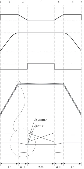
For clarity, assume the computer is initially in one of the states _|00_i, |01_i,_|10_ior_|11_iand that we wish to perform acnotgate with qubit 1 (the left qubit) as the control. The necessary profiles are shown in Fig. 2.2. Step one is to break the degeneracy of the two qubits’ energy levels to allow the control and target qubits to be distinguished. To make qubit 1 the control, the value ofA1 is increased (qubit 1 will be assumed to be the control qubit for the remainder of the chapter).

Step two is to gradually apply a positive potential to the J-electrode in order to force greater overlap of the donor electron wave functions and hence greater (indirect) coupling of the underlying nuclear qubits. The rate of this change is limited so as to be adiabatic — qubits initially in energy eigenstates remain in energy eigenstates throughout this step. This point shall be discussed in more detail shortly.

Let_|symm_iand_|anti_idenote the standard symmetric and antisymmetric superpositions of_|10_i and_|01_i. Step three is to adiabatically reduce theA1 coupling back to its initial value once more. During this step, anti-level-crossing behavior changes the input states_|10_{i → |}symm_iand_|01_{i → |}anti_i. Step four is the application of an oscillating field Bac resonant with the |symm_{i ↔ |}11_i transition. This oscillating field is maintained until these two states have been interchanged. Steps five to seven are the time reverse of steps one to three. Note that steps one and seven (the increasing and

(47)

2.2. Adiabatic cnotpulse profiles 29

decreasing ofA1) appear instantaneous in Fig. 2.2 as the only limit to their speed is that they be done in a time much greater than ¯h/0.01eV_∼ 0.1ps where 0.01eV is the orbital excitation energy of the donor electron.

In principle, the adiabatic steps should be performed slowly to achieve maximum fidelity. In practice, slow gates are more vulnerable to decoher-ence. To resolve this conflict, consider the degree to which the evolution of a given H(t) deviates from perfect adiabaticity [149]

Ignoring decoherence for the moment, for high fidelity it is necessary that Θ(t) _≪ 1. The states _|ψa(t)i are the eigenstates of H(t). To a certain

extent, it is possible to reduce Θ(t) without increasing the duration of a step by optimizing the profiles of the adiabatically varying parameters in H(t). In the case of the adiabatic Kane cnot, this means optimizing the profiles ofA1(t) andJ(t).

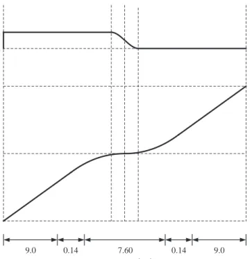
Various profiles for the adiabatic steps in thecnotprocedure have been investigated in [150]. In Fig. 2.3, we have plotted three possibleJ(t) profiles for step two of the cnot gate. The function Θ(t) for each profile is shown in Fig. 2.4. Profile 1 is a simple linear pulse. Profile 2 can be seen to be the best of the three and is described byJ(t) = 810α(1₋sech(5t/τ)) where τ = 9µs is the duration of the pulse andα = 1.0366 is a factor introduced to ensure thatJ(τ) = 810. The third profile

J(t) =      Jmax 2 t(1+π/2) τ , 0< t < τ /(1 +π/2) Jmax 2 h 1 + sinπ₂t−_{τ /}τ /₍₁₊₂(1+_/ππ/₎2)i, τ /(1 +π/2)< t < τ (2.6)

(48)

pre-1.703 1.683 810 0 10-3 0 A1 J Bac Tesla Energy Energy -2500 -3200 Energy 6 0 -6 Energy |11> |10> |01> |00> |symm> |anti> (t) 9.0 0.14 7.60 0.14 9.0 s µ Step times( ) 2 3 4 5 6 1 7 Step (t) (t)

Fig. 2.2: Gate profiles and state energies during acnotgate in units ofg_nµ_nB_z= 7.1×10−5

(49)

2.2. Adiabatic cnotpulse profiles 31 0 100 200 300 400 500 600 700 800 900 0 1 2 3 4 5 6 7 8 9 J Time Profiles linear cosh linsin

Fig. 2.3: Possible forms of the J(t) profile for step 2 of the adiabatic cnot gate. J(t) is in units ofgnµnBz= 7.1×10−5meV.

sented in this chapter due to numerical difficulties in solving the Schr¨odinger equation for profile 2. The advantage of the second two profiles over the lin-ear one is that they flatten out as J approaches 810. At J = 816.65, the system undergoes a level crossing. To maintain adiabatic evolution, J(t) needs to change more slowly near this value. Note that the reason it is desirable to makeJ(t) so large is to ensure that there is a large energy dif-ference between _|symm_i and _|anti_i during step 4 (the application of Bac). This difference is given by

δE= 2A2( 1

µBBz+gnµnBz −

1

µBBz+gnµnBz−2J

). (2.7)

Without a large energy difference, the oscillating field Bac which is set to resonate with the transition _|symm_{i ↔ |}11_i will also be very close to res-onant with _|anti_{i ↔ |}11_i causing a large error during the operation of the cnot gate. This source of error can be further reduced by using a weaker Bac at the cost of slower gate operation.

(50)

0 0.01 0.02 0.03 0.04 0.05 0.06 0.07 0 1 2 3 4 5 6 7 8 9 Omega Time Adiabatic exponential linear sinusoidal

Fig. 2.4: The adiabatic measure Θ(t) for each J(t) profile.

overall fidelity of the gate in a time of less than a micro-second with a linear pulse profile.

The above steps were simulated using an adaptive Runge-Kutta routine to solve the density matrix form of the Schr¨odinger equation

˙

ρ(t) = 1

i¯h[H(t), ρ(t)] (2.8)

in the computational basis_|n1e1n2e2i. The times used for each stage were as follows stage duration (µs) 2 9.0000 3 0.1400 4 7.5989 5 9.0000 6 0.1400

Note that the precision of the duration of stage 4 is required as the oscillating field Bac induces the states |11i and |symmi to swap smoothly

(51)

2.3. Intrinsic dephasing and fidelity 33

back and forth. The duration 7.5989µsis the time required for one swap at Bac = 10−3T.

The other step times were obtained by first setting them to arbitrary values (_∼5µs) and increasing them until the gate fidelity ceased to increase. The step times were then decreased one by one until the fidelity started to decrease. As such, the above times are the minimum time in which the maximum fidelity can be achieved. This maximum fidelity was found to be 5_×10−5 for all computation basis states.

2.3 Intrinsic dephasing and fidelity

In this chapter and Chapter 3, dephasing is modelled as exponential decay of the off diagonal components of the density matrix. While a large variety of more detailed dephasing models exist [151, 152, 153, 154, 155, 156], the chosen method is consistent with the observed experimental behavior of dephasing in solid-state systems [142]. The donor electrons and phosphorous nuclei are assumed to dephase at independent rates. With the inclusion of dephasing terms, Eq. (2.8) becomes

˙ ρ = 1 i¯h[H, ρ] −Γe[σez1,[σ z e1, ρ]]−Γe[σ z e2,[σ z e2, ρ]] −Γn[σzn1,[σ z n1, ρ]]−Γn[σ z n2,[σ z e2, ρ]]. (2.9)

To understand the effect of each double commutator, it is instructive to consider the following simple mathematical example :

˙

(52)

   ˙ m11 m˙12 ˙ m21 m˙22    =    0 ₋4Γm12 −4Γm21 0       m11(t) m12(t) m21(t) m22(t)    =    m11(0) m12(0)e−4Γt m21(0)e−4Γt m22(0)   . (2.10)

Thus each double commutator in Eq. (2.9) exponentially decays its asso-ciated off diagonal elements with characteristic time τe = 1/4Γe or τn =

1/4Γn.

For each initial state_|00_i, _|01_i,_|10_i and _|11_i, Eq. (2.9) was solved for a range of values ofτe and τnusing the pulse profiles described in Section 2.2

allowing a contour plot of the gate error versusτe and τn to be constructed

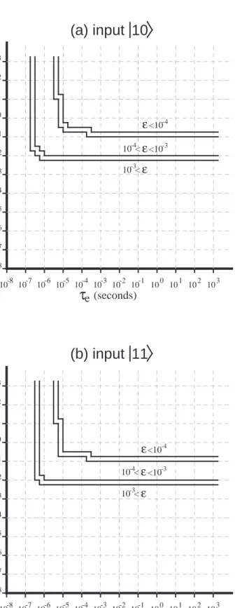
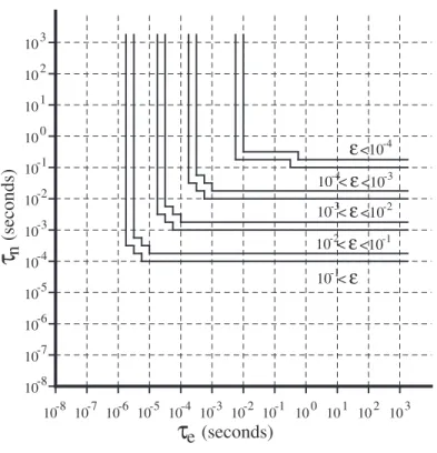
(Figs 2.5–2.6). Note that each contour is a double line as each run of the simulation required considerable computational time and the data available does not allow finer delineation of exactly where each contour is. The worst case error of all input states as a function ofτe and τn is shown in Fig. 2.7.

2.4 Conclusion

Fig. 2.7 suggests that it would be acceptable for the dephasing times of the phosphorus donor electron and nuclei to be 10ms and 0.5s respectively if a cnotreliability of 10−4 was desired. Given that the current best estimate of the donor electron dephasing time is 60ms [138], and assuming that the nuclear dephasing time is at least a factor of 80 longer again, as for the case of the relaxation times, it would be acceptable for the presence of the silicon dioxide barrier, gate electrodes, and other control structures to reduce the dephasing times by a factor of 6 without impacting on the desired reliability of the gate.

(53)

2.4. Conclusion 35 -8 -7 -6 -5 -4 -3 -2 -1 0 1 2 3 10 10 10 10 10 10 10 10 10 10 10 10 -8 10 -7 10 -6 10 -5 10 -4 10 -3 10 -2 10 -1 10 0 10 1 2 3 10 10 10

τ

e (seconds) ε<10-4 10-4<ε<10-3 10-1<ε 10-3<ε<10-2 10-2<ε<10-1

τ

n (seconds) -8 -7 -6 -5 -4 -3 -2 -1 0 1 2 3 10 10 10 10 10 10 10 10 10 10 10 10 -8 10 -7 10 -6 10 -5 10 -4 10 -3 10 -2 10 -1 10 0 10 1 2 3 10 10 10 ε<10-4 10-4<ε<10-3 10-1<ε

τ

e (seconds)

τ

n (seconds) 10-3<ε<10-2 10-2<ε<10-1

(b) input 01

(a) input 00

Fig. 2.5: Probability of errorε during acnot gate as a function of τ_e and τ_n for input state (a)|00iand (b)|01i. The first qubit is the control.

(54)

-8 -7 -6 -5 -4 -3 -2 -1 0 1 2 3 10 10 10 10 10 10 10 10 10 10 10 10 -8 10 -7 10 -6 10 -5 10 -4 10 -3 10 -2 10 -1 10 0 10 1 2 3 10 10 10 ε<10-4 10-4<ε<10-3 10-3<ε

τ

e (seconds)

τ

e (seconds) -8 -7 -6 -5 -4 -3 -2 -1 0 1 2 3 10 10 10 10 10 10 10 10 10 10 10 10 -8 10 -7 10 -6 10 -5 10 -4 10 -3 10 -2 10 -1 10 0 10 1 2 3 10 10 10 ε<10-4 10-4<ε<10-3 10-3<ε

τ

e (seconds)

τ

n (seconds)

(b) input 11

(a) input 10

Fig. 2.6: Probability of error εduring acnot gate as a function of τ_e andτ_n for input state (a) |10iand (b)|11i. The first qubit is the control.

(55)

2.4. Conclusion 37 -8 -7 -6 -5 -4 -3 -2 -1 0 1 2 3 10 10 10 10 10 10 10 10 10 10 10 10 -8 10 -7 10 -6 10 -5 10 -4 10 -3 10 -2 10 -1 10 0 10 1 2 3 10 10 10

ε

<10-4 10-4<

ε

<10-3 10-1<

ε

τ

_{e (seconds)}

τ

n (seconds) 10-3<

ε

<10-2 10-2<

ε

<10-1

Fig. 2.7: The worst case probability of errorεduring acnotgate as a function of τeandτn for all input states.

implementing gates in the Kane architecture have been devised [144], though they are slightly more vulnerable to decoherence [157]. An interesting avenue of further work would be to similarly analyze 2-qubit gates in the context of three electron spin encoded qubits which enable arbitrary computations to be performed utilizing the exchange interaction only [158], thereby elim-inating the need for oscillating magnetic fields and resulting in much faster gates.

(56)

(57)

3. Adiabatic Kane single-spin readout

Meaningful quantum computation can not occur without qubit readout. In this chapter, we assess the viability of the adiabatic Kane single-spin read-out proposal [93] when dephasing and other effects such as finite exchange coupling control are taken into account. We find that there are serious bar-riers to the implementation of the proposal, and briefly review alternatives under active investigation.

The evolution of the hyperfine and exchange interaction strengths re-quired to implement readout is reviewed in Section 3.1. The performance of the scheme is described in Section 3.2. Section 3.3 summaries our results and points to alternative approaches to readout.

3.1 Adiabatic readout pulse profiles

The geometry of the adiabatic Kane readout proposal is shown in Fig. 3.1. The basic idea is to raiseA1to distinguish the qubits, and apply appropriate voltages to induce the evolution of the hyperfine and exchange interaction strengths as shown in Fig. 3.2. This evolution passes through a level crossing resulting in the conversion of states [141]

|↓↓i |11_{i → |↓↓i |}11_i, (3.1) |↓↓i |10_{i → |↓↓i |}sni, (3.2)

(58)

Si

28

e

₁

e

₂

n

1

n

2 z

B

~2

T

T~100mK

barrier SiO₂

A

₁

J

A

₂

SET

Fig. 3.1: Geometry of adiabatic Kane readout.

|↓↓i |01_{i → |}aei|11i, (3.3)

|↓↓i |00_{i → |}aei|ani, (3.4)

where_|↓i denotes a spin-down electron, _|aei denotes the antisymmetric

su-perposition of the two electrons, and similarly for_|sni and |ani. Note that

if qubit 1 is in state_|1_i (_|0_i) the final electron state will be _|↓↓i(_|aei).

By converting the nuclear spin information into electron spin information in this manner, in principle we can apply a potential difference to theA1and A2-electrodes and, by virtue of the Pauli exclusion principle, use the SET (single electron transistor) to observe tunnelling of electron 1 onto donor 2 if and only if the nuclear spin was _|0_i.

3.2 Readout performance

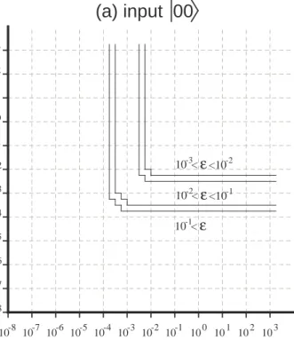
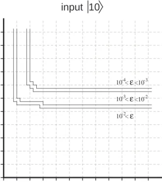
In exactly the same manner as Chapter 2, the performance of the adiabatic state conversion stage of readout was simulated with variable nuclear and electronic dephasing times τn and τe. The results of these simulations are

shown in Figs. 3.3–3.4 and show strong dependence on the initial computa-tional basis state. Indeed, we found the basis state _|11_i to be immune to

(59)

3.2. Readout performance 41 1.703 1.683 816.65 0 A1 J Energy Energy 9.0 0.14 7.60 0.14 9.0 s µ Step times( ) 2 3 4 1 Step (t) (t) 1633.3