University of South Florida University of South Florida
Scholar Commons
Scholar Commons
Graduate Theses and Dissertations Graduate School
2-12-2010
Topology Control in Wireless Sensor Networks
Topology Control in Wireless Sensor Networks
Pedro Mario Wightman Rojas University of South Florida
Follow this and additional works at: https://scholarcommons.usf.edu/etd
Part of the American Studies Commons
Scholar Commons Citation Scholar Commons Citation
Wightman Rojas, Pedro Mario, "Topology Control in Wireless Sensor Networks" (2010). Graduate Theses and Dissertations.
Topology Control in Wireless Sensor Networks
by
Pedro Mario Wightman Rojas
A dissertation submitted in partial fulfillment of the requirements for the degree of
Doctor of Philosophy
Department of Computer Science & Engineering College of Engineering
University of South Florida
Major Professor: Miguel A. Labrador, Ph.D. Rafael Perez, Ph.D. Kenneth Christensen, Ph.D. Wilfrido Moreno, Ph.D. William R. Stark, Ph.D. Date of Approval: February 12, 2010
Keywords: Network Topology, Topology Construction, Topology Maintenance, Connectivity, Sensing Coverage, Connected Dominating Set
To my three muses Astrid, Hillary and Sophia because all of you inspire me to be a little bit better every day, and to Mother Nature for the awesome job she does with her trees
Acknowledgements
The last five years have been part of an experience in which I have gratefully had the opportunity to grow not only as a professional but as a human being.
I will start by thanking my mentor and adviser Dr. Miguel Labrador, who has guided and supported me throughout these years with admirable patience, and who also has become a good friend. Thanks also to all the staff at the Department of Computer Science and Engineering at USF and Universidad del Norte which have been always there for me. Thanks to my committee Dr. Christensen, Dr. Moreno, Dr. Perez and Dr. Stark for ac-cepting my invitation to be part of this experience and for their valuable comments and suggestions.
My deepest gratitude to my wife Hillary and my beloved daughter Sophia, whose love, patience and support have helped to keep me on the right track. I extend this gratitude especially to my mother for her unconditional love, and to my parents-in-law without whose help I would not have had the opportunity to finish this dissertation.
Thanks to all my friends who I no longer consider just friends, because we have become more like a family: thanks to Dala, Migue, and all the people from the Information Sys-tems Lab for their support and the good laughs. Special thanks to Aldo whose help was critical in these final months and to Alcides for the name of the simulator, among other excellent suggestions.
Finally, and most importantly, I thank God for giving me the opportunity to grow and improve myself in order to be able to serve better.
Table of Contents
List of Tables vii
List of Figures viii
Abstract xiii
Chapter 1 Introduction 1
1.1 Wireless Sensor Networks 2
1.2 Topology Control 5
1.2.1 Network Topology 5
1.2.2 Definition of Topology Control 8
1.3 Problem Statement 11
1.4 Contributions 15
1.5 Structure of the Dissertation 17
Chapter 2 Literature Review 19
2.1 Topology Control Taxonomy 20
2.1.1 Topology Construction Taxonomy 21
2.1.2 Topology Maintenance Taxonomy 22
2.2.1 Controlling the Transmission Power 24 2.2.1.1 Centralized Approaches 24 2.2.1.2 Distributed Approaches 29 2.2.1.3 Heterogeneous Devices 32 2.2.2 Hierarchical Techniques 33 2.2.2.1 Backbone-based Techniques 34 2.2.2.2 Cluster-based Techniques 43 2.2.2.3 Adaptive Techniques 44 2.2.3 Hybrid Approaches 44
2.3 Coverage-oriented Topology Construction 45
2.3.1 Classification Factors 46
2.3.1.1 Definition of the Area of Interest 47
2.3.1.2 Redundancy 48
2.3.2 Other Considerations in Coverage-oriented Topology
Construction Protocols 49
2.3.3 Examples of Coverage-oriented Topology Construction
Protocols 50
2.4 Topology Maintenance 61
2.4.1 Classification Factors 62
2.4.1.1 Selection Policy: Static, Dynamic and
Hy-brid 62
2.4.1.2 Level of Involvement: Global and Local 65
2.4.2 Examples of Topology Maintenance Algorithms 68
Chapter 3 Methodology 72
3.1 An Analytical Solution to the MCDS Problem 72
3.2 The MIP Approach for the Minimum Connected Dominating
Set Problem 77
3.3 Performance Evaluation: Assumptions, Metrics, Factors and
Levels 82
3.3.1 Assumptions 82
3.3.2 Performance Metrics 83
3.3.3 Factors and Levels 84
3.3.4 Energy Model 86
Chapter 4 The A3 and A3Lite Topology Construction Protocols for
Connectiv-ity 88
4.1 Introduction 89
4.2 The A3 Algorithm 90
4.2.1 The Neighborhood Discovery Process 91
4.2.2 Children Selection Process 92
4.2.3 Second Opportunity Process 94
4.2.3.1 The Selection Metric 96
4.3 The A3Lite Algorithm 98
4.3.1 The Neighborhood Discovery Process 98
4.3.2 Children Selection Process 99
4.4.1 Experiment 1: Changing the Node Degree 102
4.4.2 Experiment 2: Changing the Node Density 105
4.4.3 Experiment 3: Ideal Grid Topologies 108
Chapter 5 The A3Cov and A3CovLite Topology Construction Protocols for
Coverage 111
5.1 The A3Cov Algorithm 112
5.2 The A3CovLite Algorithm 116
5.3 Theα-Coverage Sensing Coverage Definition 116
5.4 Performance Evaluation 119
5.4.1 Comparison with Theoretical Deployments 120
5.4.1.1 Experiment 1: Same Radii 123
5.4.1.2 Experiment 2: Different Radii 128
5.4.1.3 Experiment 3: Differentα-coverage 132
5.4.2 Comparison with Distributed Protocols 138
5.4.2.1 Comparison With ACOS 138
5.4.2.2 Comparison With StanGA 143
Chapter 6 Topology Maintenance Protocols 146
6.1 Introduction 146
6.2 Static Global Topology Rotation 147
6.3 Dynamic Global Topology Recreation 148
6.4 Dynamic Local - DSR 149
6.6 Performance Evaluation 153 6.6.1 Performance Evaluation of Static Global Topology
Maintenance Techniques 155
6.6.1.1 Sparse Networks 156
6.6.1.2 Dense Networks 160
6.6.2 Performance Evaluation of Dynamic Global Topology
Maintenance Techniques 161
6.6.2.1 Sparse Networks 163
6.6.2.2 Dense Networks 164
6.6.3 Performance Evaluation of Dynamic Local Topology
Maintenance Techniques 168
6.6.3.1 Sparse Networks 169
6.6.3.2 Dense Networks 169
6.6.4 Performance Evaluation of Hybrid Global Topology
Maintenance Techniques 171
6.6.4.1 Sparse Networks 174
6.6.4.2 Dense Networks 174
6.7 Comparison of Topology Maintenance Techniques 176
6.8 Sensitivity Analysis 181
6.8.1 Time-based Analysis 182
6.8.2 Energy-based Analysis 184
6.8.3 Density-based Analysis 186
7.1 Conclusions 191
7.2 Summary of Contributions 193
7.3 Future Work 195
List of References 197
Appendices 210
Appendix A: A Brief Overview of Atarraya 211
List of Tables
Table 3.1 Parameters for the energy model. 87
Table 4.1 Simulation parameters for connectivity-oriented protocols. 101
Table 5.1 Simulation parameters for coverage-oriented protocols. 121
Table 5.2 Radii and topology sizes for coverage-oriented protocols. 123 Table 6.1 Simulation parameters for topology maintenance protocols. 154
List of Figures
Figure 1.1 Diagram of components of a wireless sensor device. 2
Figure 1.2 Example of a network architecture that includes a wireless sensor
network. 3
Figure 1.3 Comparison of topologies: the MaxPowerGraph versus the reduced
topology. 7
Figure 1.4 Diagram that models the iterative execution of a topology control
algorithm. 11
Figure 2.1 General taxonomy for topology control protocols. 21
Figure 2.2 Taxonomy of connectivity-oriented topology construction protocols. 24 Figure 2.3 Topology control by reducing the number of active nodes and the
creation of a network backbone. 35
Figure 2.4 Growing a tree with 1-hop neighbor information. 37
Figure 2.5 Classification of coverage-oriented topology construction protocols. 46 Figure 2.6 Different deployment geometries for connected coverage topologies
withRS=RC. 52
Figure 2.7 Example of original and modified solutions of the circle packing
problem. 56
Figure 2.8 Theoretical comparison between the packing problem and the optimal
deployments. 57
Figure 2.10 Classification of topology maintenance. 68
Figure 3.1 Examples of MDS solutions. 73
Figure 3.2 Example of the “flow of tokens” technique. 79
Figure 4.1 The A3 algorithm. 91
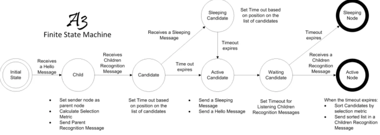
Figure 4.2 The A3 protocol finite state machine. 92
Figure 4.3 The A3Lite protocol finite state machine. 98
Figure 4.4 Results of experiment 1: changing the node degree. 103
Figure 4.5 Results of experiment 2: changing the node density. 106
Figure 4.6 Square grids deployment. 108
Figure 4.7 Results of experiment 3: ideal grid topologies. 110
Figure 5.1 The A3Cov protocol finite state machine. 113
Figure 5.2 The A3CovLite protocol finite state machine. 115
Figure 5.3 Example ofα-coverage. 117
Figure 5.4 Performance in sparse networks whenRComm=RSense. 125
Figure 5.5 Performance in dense networks whenRComm=RSense. 126
Figure 5.6 Performance in sparse networks whenRComm>RSense. 129
Figure 5.7 Performance in dense networks whenRComm>RSense. 130
Figure 5.8 Performance in sparse networks whenRComm>RSenseandα>1. 133
Figure 5.9 Performance in dense networks whenRComm>RSenseandα>1. 134
Figure 5.10 Performance in sparse networks whenRComm>RSenseandα<1. 136
Figure 5.12 Performance of the A3Cov and A3CovLite protocols in sparse
net-works with different radii andα-coverage parameter. 139
Figure 5.13 Performance of the A3Cov and A3CovLite protocols in dense
net-works with different radii andα-coverage parameter. 140
Figure 5.14 Comparison of performance of the A3Cov, A3CovLite protocols and
the ACOS protocol for 800 nodes. 142
Figure 5.15 Comparison of performance of the A3Cov, A3CovLite protocols and
the StanGA protocol for different coverage configurations. 144 Figure 6.1 Phase one of the DSR-based dynamic local topology maintenance
technique. 151
Figure 6.2 Network lifetime with and without static global topology maintenance using the A3, EECDS, and CDS-Rule-K topology construction
mech-anisms in sparse networks. 158
Figure 6.3 Best performing static global topology maintenance techniques in
sparse networks. 159
Figure 6.4 Network lifetime with and without static global topology maintenance using the A3, EECDS, and CDS-Rule-K topology construction
mech-anisms in dense networks. 162
Figure 6.5 Best performing static global topology maintenance techniques in
dense networks. 163
Figure 6.6 Network lifetime with and without dynamic global topology mainte-nance using the A3, EECDS, and CDS-Rule-K topology construction
mechanisms in sparse networks. 165
Figure 6.7 Best performing dynamic global topology maintenance techniques in
sparse networks. 166
Figure 6.8 Network lifetime with and without dynamic global topology mainte-nance using the A3, EECDS, and CDS-Rule-K topology construction
mechanisms in dense networks. 167
Figure 6.9 Best performing dynamic global topology maintenance techniques in
Figure 6.10 Network lifetime with and without dynamic local topology mainte-nance using the A3, EECDS, and CDS-Rule-K topology construction
mechanisms in sparse networks. 170
Figure 6.11 Best performing dynamic local topology maintenance techniques in
sparse networks. 171
Figure 6.12 Network lifetime with and without dynamic local topology mainte-nance using the A3, EECDS, and CDS-Rule-K topology construction
mechanisms in dense networks. 172
Figure 6.13 Best performing dynamic local topology maintenance techniques in
dense networks. 173
Figure 6.14 Network lifetime with and without hybrid global topology mainte-nance techniques using the A3, EECDS, and CDS-Rule-K topology
construction mechanisms in sparse networks. 175
Figure 6.15 Best performing hybrid global topology maintenance techniques in
sparse networks. 176
Figure 6.16 Network lifetime with and without hybrid global topology mainte-nance techniques using the A3, EECDS, and CDS-Rule-K topology
construction mechanisms in dense networks. 177
Figure 6.17 Best performing hybrid global topology maintenance techniques in
dense networks. 178
Figure 6.18 Best performing topology maintenance techniques in sparse and
dense networks. 179
Figure 6.19 Time-based sensitivity analysis of network lifetime for static,
dy-namic, and hybrid topology maintenance techniques. 183
Figure 6.20 Best performing techniques out of time sensitivity tests. 184 Figure 6.21 Energy-based sensitivity analysis of network lifetime for static,
dy-namic, and hybrid topology maintenance techniques. 185
Figure 6.23 Node density-based sensitivity analysis of network lifetime for static,
dynamic, and hybrid topology maintenance techniques. 187
Figure 6.24 Best performing techniques out of the density sensitivity tests. 189 Figure 6.25 Comparison of network lifetime when using topology construction
and maintenance, topology construction only and no topology
con-trol. 190
Figure A.1 Atarraya’s functional components. 213
Figure A.2 Useful diagrams to design a communication protocol. 243
Figure A.3 Simulation control panel. 247
Figure A.4 Other protocols for educational purposes. 249
Figure A.5 Different topology designs generated by Atarraya. 256
Figure A.6 Deployment definition panel. 257
Figure A.7 Other parameters for deployment definition. 261
Figure A.8 Example of statistics generated by Atarraya. 264
Figure A.9 Report panel. 265
Figure A.10 Node statistics panel. 266
Figure A.11 Main window description. 267
Topology Control in Wireless Sensor Networks Pedro Mario Wightman Rojas
ABSTRACT
Wireless Sensor Networks (WSN) offer a flexible low-cost solution to the problem of event monitoring, especially in places with limited accessibility or that represent danger to humans. WSNs are made of resource-constrained wireless devices, which require en-ergy efficient mechanisms, algorithms and protocols. One of these mechanisms is Topol-ogy Control (TC) composed of two mechanisms, TopolTopol-ogy Construction and TopolTopol-ogy Maintenance.
This dissertation expands the knowledge of TC in many ways. First, it introduces a com-prehensive taxonomy for topology construction and maintenance algorithms for the first time. Second, it includes four new topology construction protocols: A3, A3Lite, A3Cov and A3LiteCov. These protocols reduce the number of active nodes by building a Con-nected Dominating Set (CDS) and then turning off unnecessary nodes. The A3 and A3-Lite protocols guarantee a connected reduced structure in a very energy efficient manner. The A3Cov and A3LiteCov protocols are extensions of their predecessors that increase the sensing coverage of the network. All these protocols are distributed –they do not require localization information, and present low message and computational complexity. Third, this dissertation also includes and evaluates the performance of four topology maintenance protocols: Recreation (DGTRec), Rotation (SGTRot), Rotation and Recre-ation (HGTRotRec), and Dynamic Local-DSR (DLDSR).
Finally, an event-driven simulation tool named Atarraya was developed for teaching, researching and evaluating topology control protocols, which fills a need in the area of topology control that other simulators cannot. Atarraya was used to implement all the topology construction and maintenance cited, and to evaluate their performance. The re-sults show that A3Lite produces a similar number of active nodes when compared to A3, while spending less energy due to its lower message complexity. A3Cov and A3CovLite show better or similar coverage than the other distributed protocols discussed here, while preserving the connectivity and energy efficiency from A3 and A3Lite. In terms of net-work lifetime, depending on the scenarios, it is shown that there can be a substantial in-crease in the network lifetime of 450% when a topology construction method is applied, and of 3200% when both topology construction and maintenance are applied, compared to the case where no topology control is used.
Chapter 1: Introduction
Data is today’s gold: finding new sources, new ways to gather it and new kinds of conclu-sions to draw from it are becoming very attractive research areas with countless applica-tions in the world. In the time you spent reading this dissertation, billions of bits will be generated with the only purpose of gathering data about virtually everything: how many cars are crossing the Skyway bridge in St. Petersburg, FL, the temperature on each floor of the Empire State building in New York city, or the current location of a group of zebras in the savannas of Central Africa, and this is just the beginning. However, gathering this data from places that are not easily accessible or that are dangerous to humans requires the right technology.
One technology that fits the requirements needed for a low-cost and flexible way to obtain data from virtually any location, from urban environments, to personal networks and also scenarios with limited access to communication and power infrastructures isWireless
Sensor Networks (WSNs). As it will be seen later on this chapter, these networks are made
of devices very constrained in resources, which makes it imperative for them to work in a very efficient manner, especially in terms of energy consumption. One of the ways a WSN can become more energy-efficient is by usingTopology Control (TC), which is the
main focus of this dissertation.
This chapter formally introduces the concept of Wireless Sensor Networks and Topology Control. Furthermore, this chapter explains in detail the motivations behind the use of
Figure 1.1: Diagram of components of a wireless sensor device.
WSNs and how Topology Control algorithms can improve their performance. Subse-quently, the problem statement will be introduced, accompanied by some discussion on the key study variables and procedures used in this work. After the problem statement, the chapter includes the detailed list of contributions presented in this dissertation, and finalizes with the structure of the dissertation.
1.1 Wireless Sensor Networks
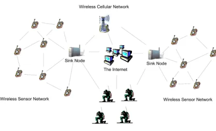
Advances in sensor and wireless communication technologies in conjunction with devel-opments in microelectronics have made available a new type of communication network made of battery-powered integrated wireless devices with sensing capabilities. Wireless Sensor Networks, as they are named, are self-configured and infrastructureless wireless networks made of small devices equipped with specialized sensors, wireless transceivers, a processing unit, a small memory unit, and a power source, which can be as small as a pair of AA batteries. A general diagram of the structure of one of these devices can be seen in Figure 1.1, taken from [1].
Figure 1.2: Example of a network architecture that includes a wireless sensor network. The main goal of a WSN is to collect data from the environment and send it to a reporting site where the data can be stored, observed and analyzed. Wireless sensor devices also respond to queries sent from a control site to perform specific instructions or provide on-demand sensing samples. Finally, wireless sensor devices can be equipped with actuators to perform actions upon certain conditions. These networks are sometimes more specifi-cally referred as Wireless Sensor and Actuator Networks.
Some of the applications in which the use of a WSN has been ideal include the moni-toring and acting upon events in dangerous or unaccessible places for humans. As such, WSNs have been installed in places such as chemical plants, to monitor poisonous gases; water plants, rivers, lakes and the like, to assess the level and quality of the water; areas with endangered species, to monitor their travel patterns and behaviors; buildings, to monitor the quality of the air and make them more energy-efficient; used by the military, to detect intruders; or used in other similar applications.
Figure 1.2 presents an example of a complete solution that integrates WSNs with other current technologies, like the cellular network, the Internet, and other wireless ad hoc
technologies [1]. As it can be seen, a typical structure of a WSN includes two types of wireless devices:sink nodesandregular nodes.
The sink nodes are the gateways of the WSN: all data generated from the sensor network will be gathered at the sink node and transmitted to the control site using a secondary communication interface, like Ethernet, cellular , satellite or another wireless network. Furthermore, the sink nodes also allow information from outside into the WSN, like com-mands, updates or queries. In some cases, the sink nodes also play the role of organizers of the network, keeping track of the state of the nodes and address assignation, or by being the initiators of the maintenance procedures.
The regular nodes are the gross majority in the network; they are in charge of collecting all the data about the variables being monitored and of reporting it to the sink node. In addition, if the network is large enough that some devices cannot reach the sink node directly, the regular nodes must provide multi-hop forwarding of the data, so that even the farthest nodes can send their data to the sink node. Due to the critical responsibilities of the sink nodes, they often have a better configuration in terms of processing, memory and, mainly, energy, when compared to the regular nodes; in other words, when every regular node can fail, the sink nodes are expected not to.
Even though the application domain of WSNs has been restricted to simple data-oriented monitoring and reporting applications, especially because of the energy constrained char-acteristics of the current technology, new network architectures with heterogeneous de-vices and expected advances in technology are eliminating some of the current limitations and expanding the spectrum of possible applications for WSNs considerably, including more advanced functions like handling multimedia data.
However, at the present time, of all the constraints considered in most available wireless sensor devices, energy consumption is of paramount importance. This assertion can be
explained with the following two reasons: first, a single wireless device possesses a small energy source, which is expected to last several months; and second, if the network is de-ployed in an inaccessible area, changing depleted batteries is not feasible, so the wireless devices must use their already small energy source in a very efficient way. These are the main reason why most of the research on WSNs has been concentrated on the design of energy- and computationally-efficient algorithms and protocols; this interest can be measured by the large number of algorithms, techniques, and protocols that have been developed to save energy, and thereby extend the lifetime of the network. One of the most important techniques utilized to reduce energy consumption in wireless sensor networks is Topology Control.
1.2 Topology Control
1.2.1 Network Topology
Before the concept of Topology Control is introduced, as well as all its benefits for the network’s operations, it is important to start by dedicating some time to the concept of
Network Topology, which is absolutely necessary to understand the foundations and
moti-vations behind TC. A simple definition of network topology can be the following:
Network Topologyis the set of all active nodes and active links in the network
along which direct communication can occur [2].
This definition can be extended based on the concept ofGeometric Random Graphs. Let
G= (V,E,r)be a Geometric Random Graphs (GRG), in whichV is the set of vertices,E
is the set of edges, andris the radius of the transmission range of the nodes. Every vertex
and an open ball with radiusr. This open ball is a set that contains all the vertices with
distance less thanrrespective to the node, which represents the communication area of
the nodes. The nodes in the open ball are the only neighbors that the node can communi-cate with directly. The formal definition of the open ball is presented in Equation 1.1 [3] as follows:
Br(x) ={y:d(x,y)<r} (1.1)
wherex,y∈V andd(·,·)is the Euclidean distance between two nodes. The set of edgesE
are the union of all pairs created by each vertex and all the adjacent vertices contained in its open ball. Providing that communication is not always bidirectional, links are modeled as unidirectional edges. Given that the open balls of the vertices are independent, the existence of the edge(x,y)does not imply the existence of the edge(y,x). In addition,
if any metric can be calculated between a pair of adjacent nodes, i.e., distance, angle, remaining energy, etc., it can be used as the weight of the edge,w. This metric, as well
as the edges, is not always symmetric, so weights could be different from one direction to the other. The formal definition of the set of edges is presented in Equation 1.2. However, it is assumed that all networks used in this dissertation can be modeled as bidirectional graphs.
E={(x,y,w):y∈Br(x)∧w∈ℜ},x,y∈V (1.2)
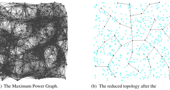
The resultant graph when all the sensors are set to transmit at their maximum power is called theMaximum Power Graph, orMaxPowergraph. This is normally the case when
the nodes have just been deployed and they are exploring their neighborhood. This graph represents the maximum topology of the network in terms of active nodes and active
(a) The Maximum Power Graph. (b) The reduced topology after the topology construction mechanism.
Figure 1.3: Comparison of topologies: the MaxPowerGraph versus the reduced topology. links. One example of this graph is shown in Figure 1.3(a), in which 500 nodes are uni-formly deployed in an area of 500m × 500mwith transmission ranges of 80m.
In terms of the organization of the a network topology, it can be predesigned by the user in the cases where manual allocation of the nodes is possible, or it can be totally random in the cases where the deployment is made by other means, i.e., the nodes are dropped from a helicopter.
In the first case, the user has total control over the topology: the user can calculate the minimum amount of required nodes and their exact positions on the area in order to per-form the task in an optimal manner. This technique is not feasible for applications in which accessibility is not possible or in a dangerous scenario where the lives of the people performing the deployment are at risk. In addition, this solution many not be feasible for large networks or when immediate availability of the network is required.
In the second case, when the topology is randomly deployed on an inaccessible area, the user lacks the power to assign exact locations to the nodes and needs a higher number of nodes in order to guarantee coverage of the area. These issues create another problems,
namely a random topology configuration that is not apt for optimal performance, which can show characteristics such as:
• There can be very dense areas in which many nodes are transmitting packets very often, generating a great amount of collisions and delays.
• The nodes may be transmitting at full power, which is not necessary to reach the next node in their path towards the sink.
• There are many nodes that, due to proximity, are sensing the same events and thus, sending redundant data to the sink.
In all of these cases, the network is wasting energy in unnecessary actions. These are the problems that Topology Control can help to prevent.
1.2.2 Definition of Topology Control
The main goal of topology control is to modify the initial maximum power topology and avoid the occurrence of the previously mentioned problems and their impact on the en-ergy consumption by altering the initial topology, while keeping important characteristics like connectivity and coverage.
If the user wants to pre-design a topology to guarantee optimality, the need of topology control is not critical and the solution of the optimal topology can be calculated off-line and replicated in reality. However, a solution of this nature should take into account the characteristics of the terrain, the radio spectrum and other variables that may affect the actual communication between nodes once they have been deployed, but sometimes that information is difficult to obtain and the permanent testing, the manual deployment and
the large number of possible combinations necessary to generate a successful output may delay the whole deployment process.
The second case is when the deployments are random topologies and the location of the nodes cannot be changed or sometimes not even determined. In this scenarios there are still two variables that the user can use to reorganize the topology: the state of activity of the nodes (active, inactive) and the radio transmission power. The first variable allow the user to reduce the number of active nodes, which has an impact on the density in certain areas, reducing interference and the generation of redundant data. Inactive nodes turn off their transceivers and go into a very low energy consumption mode, from which they can be turned on again to be part of the active network if they are needed in the future. The second variable has a direct impact on energy consumption and on the level of interfer-ence, given that radio transmission is the most expensive operation in terms of energy and one of the most commonly done; in other words, reducing the energy required to transmit a message will represent important savings.
The advantage of a random topology is that the deployment can be done relatively quick-ly, and the network may become available almost immediately. In addition, a topology control algorithm should be robust enough to take care of the characteristics of the de-ployment area. The main disadvantage of this kind of dede-ployment is that a higher amount of nodes is required in order to increase the probability of having nodes in every region of the monitored area, which has a direct impact on the cost of the network.
One example of the application of topology control can be seen in Figure 1.3(b), which shows how the MaxPower network shown in Figure 1.3(a) can be reduced after applying a TC algorithm to decrease the number of active nodes. A more formal definition of topol-ogy control can be the following:
“Topology Controlis the reorganization and management from time to time
of certain node parameters and modes of operation to modify the topology of the network, with the goal of extending its lifetime while also preserving important characteristics, such as network connectivity and sensing cover-age.” [1].
In general, TC can be seen as an iterative process, as shown in Figure 1.4, extracted from [1]. First, there is an initialization phase common to all wireless sensor network deploy-ments. In this phase, nodes discover themselves and use their maximum transmission power to build the initial topology. After this initialization phase, the second phase builds a new (reduced) topology. This phase is calledTopology Construction. The new reduced
topology will run for certain amount of time, as the participating sensors will consume their energy over time. Therefore, as soon as the topology construction phase establishes the reduced network, theTopology Maintenancephase must start working.
During this phase, a new algorithm must be in place to monitor the status of the reduced topology and trigger a topology restoration process when appropriate, that may be a pro-cess entirely defined by the maintenance protocol itself or that may include the invocation of the topology construction algorithm. Over the lifetime of the network, it is expected that this cycle will be repeated many times until the energy of the network is depleted. There are many different algorithms that can be used in the topology construction and maintenance phases. In this dissertation, new topology construction and topology mainte-nance protocols will be introduced.
Figure 1.4: Diagram that models the iterative execution of a topology control algorithm. 1.3 Problem Statement
The outcome seen in Figure 1.3(b) looks very simple:“Yes, it’s a tree that covers
ev-eryone. So, is that all?”, well, let the following explanation show why the problem of
topology control is not as simple as it looks.
First of all, the algorithms and protocols should run in a distributed manner, so they can be implemented in large networks. Second, topology construction algorithms and proto-cols must have a low computational and message complexity, so they can be efficiently run in computationally weak devices and not drain the nodes’ batteries. Third, it is de-sirable that the algorithms are able to run without the help of additional hardware like GPS devices or localization mechanisms, so low cost is maintained and no additional energy is spent. Finally, the topology construction algorithm must produce a connected network that will cover the area of interest with a minimum number of nodes, while the topology maintenance algorithms must guarantee that the resources of the network are used effectively in order to keep the network active the longest possible time. All these constraints combined make the design and implementation of simple distributed topology control algorithms a very challenging problem.
In order for these processes to be effective and provide the expected results in terms of extending the lifetime of the network, both topology construction and maintenance mech-anisms must be designed with careful consideration of the following requirement aspects:
• Distributed algorithm:Centralized topology control mechanisms need global
infor-mation and therefore are very expensive when implemented.
• Local information:Nodes should be able to make topology control decisions
lo-cally. This reduces the energy costs and makes the mechanism scalable.
• Location information:The need of extra hardware, like GPS devices, or support
mechanisms like localization protocols add to the cost in terms of dollars and en-ergy consumption.
• Connectivity:The reduced network must be connected, so all active nodes can
exchange messages among themselves as well as with the sink node.
• Coverage:The reduce topology must cover the area of interest despite the number
of active nodes.
• Small node degree: A small node degree means a small number of neighbors, which
may produce a lower number of collisions and retransmissions, saving energy.
• Link bidirectionality: Bi-directional links facilitate the proper operation of some
Medium Access Control (MAC) layer protocols, such as the one utilized by the IEEE 802.11 standard, which sends Request-To-Send (RTS) and Clear-To-Send (CTS) signals and also acknowledgments in the return path.
• Simplicity:Topology control algorithms must have a low computational complexity,
• Low message complexity:Topology control mechanisms must work with very low
message overhead, so they are energy-efficient and can be run many times as part of the topology control cycle.
• Energy-efficiency: All the factors considered thus far and those discussed in the last
section converge in the issue of energy-efficiency, which is essential for topology control mechanisms and wireless sensor networks in general.
• Energy awareness:The decision making process in the selection of the reduced
topology must be aware of the nodes’s remaining energy in order to avoid giving responsibilities to weak nodes that can jeopardize the activity of the network.
• Spanner:The reduced topology should be a spanner of the Unit Disk Graph in
terms of both length and number of hops. A subgraphG0is a spanner of a graph
Gfor length (number of hops) if there is a positive real constantxsuch that for any
two nodes, the length (number of hops) of the shortest path inG0is at mostxtimes
of the length (number of hops) of the shortest path inG. The constantxis called the
length (number of hops) stretch factor.
• Convergence time: The topology construction and maintenance processes should
take place as fast as possible and converge after a limited number of steps.
• Memory consumption:Wireless sensor devices often have a small amount of
ory. Some topology control techniques may require considerable amounts of mem-ory, such as those that store pre-calculated topologies.
• Even energy distribution: Topology control techniques should somehow try to
network. The topologies should be changed so that all nodes have a similar partici-pation in the network.
This dissertation presents new topology control mechanisms that work considering these aspects. All the topology construction protocols proposed in this document work by find-ing a minimum set of active nodes, that provides a connected network that is able to per-form all the tasks required by the user, whether connectivity or coverage, while turning all the rest of the nodes off to save their energy for future maintenance of the active topology. The calculation of this set of special nodes is modeled using the Minimum Connected Dominating Set (MCDS) problem for communication tasks, and the Minimum Connected Sensing Coverage (MCSC) problem for connectivity and coverage, which will be ex-plained in detail in the next chapter.
The main reason why this methodology was selected is that, next to radio transmission, idle listening is the most costly operation of a node. This means that, if all the nodes are kept awake and the only change is made to the transmission power, the idle listening time from the entire network will still decrease the amount of saved energy; plus the fact that the problem of redundant sensing is still present, which will increase the load of the network with no need.
In the proposed solutions of this work, all redundant nodes have their transceivers turned off, so no energy is wasted in idle mode and unnecessary redundancy is reduced. The hypothesis is that the algorithms proposed in this dissertation, while creating minimal message overhead compared to their counterparts, can reduce and maintain an active topology, extending the lifetime of the network, while keeping radio connectivity and sensing coverage of the deployment area.
1.4 Contributions
The contributions presented in this dissertation are the following:
• New taxonomies for topology control, topology construction and topology
mainte-nance algorithms.Based on the new definition of topology control, which
differ-entiates the construction and maintenance processes, a new taxonomy for topol-ogy control algorithms was proposed in order to integrate and extend the current algorithms presented in [2, 4, 5] which focus only on the first process. The main contribution in this area is the definition of a taxonomy for topology maintenance algorithms for the first time, which none of the cited works include. In addition, some modifications were performed on the existing taxonomies, in order to include special branches to topology construction protocols for heterogeneous networks and coverage-oriented protocols.
• The A3 family of simple topology construction algorithms. In this dissertation, four
new topology construction algorithms are introduced: A3, A3Lite, A3Cov and A3CovLite. These protocols calculate aConnected Dominating Set (CDS)on the
initial MaxPower topology, leaving in active state only the dominating nodes which provide connectivity and coverage in the network, and turning off all dominated (redundant) nodes, which are considered unnecessary for the correct activity of the network at the time of execution. A3 is the first version of the algorithm and provides a backbone for connectivity purposes only. The initial protocol was even-tually modified into two new branches: theLiteversions and theCovversions. The
Liteversions provide a very low computational and message complexity, compared
to theNon-Litecounterparts. TheCovversions produce a reduced topology that
evaluation of these protocols is based on the comparison of average behavior in random topologies against other algorithms in the literature, and against theoretical optimal deployments.
• A set of topology maintenance algorithms.Four topology maintenance algorithms
are presented in this document: Dynamic Global Topology Recreation (DGTRec),
Static Global Topology Rotation (SGTRot),Hybrid Global Topology Recreation and
Rotation (HGTRecRot)andDynamic Local DSR, DLDSR. The first two protocols
have been proposed before in the literature, but have not been implemented in de-tail. The last two are completely new algorithms. These algorithms were designed based on the proposed taxonomy for topology maintenance algorithms. The perfor-mance evaluation of these algorithms is based on the comparison of the average results in random topologies, and working jointly with three different topology construction protocols. It is very important to mention that, to the knowledge of the author, this is the first time that a modularization of the topology constructions and maintenance protocols has been implemented for joint testing performance.
• Atarraya: a new simulation tool for teaching and researching topology control
algorithms. As a tool was needed to design and test the proposed topology
con-trol algorithms, the topology concon-trol simulatorAtarrayawas created. Atarraya
is a discrete-event simulator for evaluating topology control algorithms. It was developed in Java, which allows Atarraya to be a very portable application among different operating systems. In addition, the simulator is being offered for free to the scientific community as an open source project, based on the GNU license model. This simulator provides a friendly environment for designing both topology construction and maintenance algorithms, allowing the modularity to combine those protocols, which has not been seen in any other simulator of its kind. In addition,
it can be extended to support schemes for data aggregation, routing, node mobility and different energy models.
• A new book on topology control.Most of the work presented in this dissertation has
been included in the book“Topology Control in Wireless Sensor Networks - with a
companion simulation tool for teaching and research”, written by Miguel Labrador
and Pedro Wightman, and published in 2009 by Springer Science [1]. This book presents an integral definition of topology control, based on the decoupling of the construction and maintenance processes, and also provides the simulator Atarraya as a tool not only for researching and designing of new TC protocols, but also as a useful tool for teaching communication protocols in an user-friendly environment.
• A new mixed integer programming definition of the minimal connected dominating
set problem.Even though there has been previous definitions of the MCDS problem
in the literature, most of them depend on the separate solution of the problems of connectivity and domination, which may not necessarily guarantee an optimal joint solution, or in extensive preprocessing. This dissertation provides an def-inition of the problem based on a very simple insight of the problem that solves both connectivity and dominance in a single formulation, and does not require any preprocessing. The results of this new model are compared with the results from the approximation protocols presented in Chapter 3.
1.5 Structure of the Dissertation
The structure of the dissertation will continue as follows. Chapter 2 will be dedicated to the literature review of the problem of topology control, including the introduction to the proposed taxonomy, and references to the most important algorithms in both topology
construction and topology maintenance in the categories of the taxonomy. In addition, a section of the chapter will be dedicated to the Connected Dominating Set-based protocols for topology construction for both connectivity and coverage. Chapter 3 describes the methodology used for the performance evaluation of the different topology construction and maintenance protocols introduced in this dissertation, including both the analytical and simulation-based approaches. Chapter 4 will introduce the topology construction algorithms A3 and A3Lite, which are focused only on producing a connected topology with a minimum number of active nodes, and will show their performance evaluation against two very well known CDS-based topology construction algorithms. The A3Cov and A3CovLite topology construction algorithms will be introduced in Chapter 5, which provide not only a connected topology but a topology that covers a high degree of the de-ployment area, and will show their performance evaluation against some optimal theoret-ical deployments, theirNon-Covversions and two other coverage-oriented topology
con-struction protocols. Chapter 6 will present the topology maintenance algorithms proposed in this dissertation, including their joint performance testing with some of the topology construction algorithms presented in Chapter 4. The conclusions of this work and some final remarks will be presented in Chapter 7. In addition, a detailed description of the internal structure and use of the simulator Atarraya will be included in the Appendix A.
Chapter 2: Literature Review
The study of topology control has gained importance since the end of the previous decade, especially in wireless ad hoc and sensor networks, because of all the potential benefits in energy consumption that come with transforming the MaxPower graph into a more manageable and efficient network. Researchers in this area took advantage of the simi-larities of these networks with the random graphs on theoretical fields, in order to adopt the existing bast theory in graphs and apply it into this new kind of network.
This fact determined that the first attempts to perform topology control were based mainly in classical graph algorithms, like the minimal spanning tree, the set cover and coloring problem, just to mention some, because the were already capable of altering the original structure of a graph in order to reduce the topology.
However, most of these algorithms require global information and work in a centralized manner, which became a natural initial assumption to make in order to allow the use of these solutions. These assumptions stopped being valid very quickly for scenarios in which the size of the network made it infeasible to use a centralized solution or when global information was to expensive to obtain. This opened the horizon for the develop-ment of distributed protocols that required local information, which corresponded more with some of the real characteristics of these networks: they can reach high levels of scalability, randomness in localization of the nodes and their communication links, and global information is too costly to collect and distribute.
The amount of work in the area has been very broad and varied. As part of this work, a new taxonomy for classifying topology control protocols is presented. The new proposed taxonomy is an extension of three previous taxonomies, introduced in [2, 4, 5]. The new taxonomy, which is one of the main contribution of this work, provides a road map for the rest of this chapter.
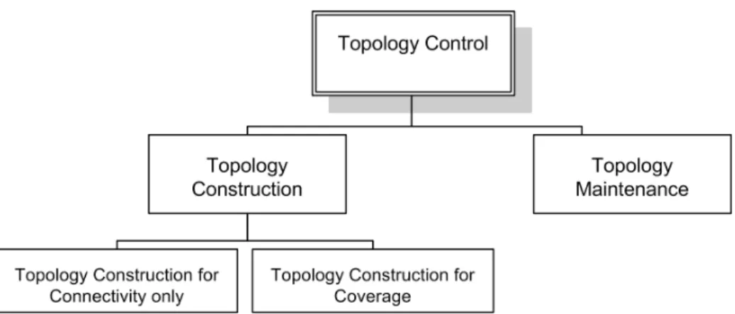
2.1 Topology Control Taxonomy
As mentioned in Chapter 1, topology control algorithms were traditionally considered as a monolithic process: reduction and maintenance were implemented as a single protocol. The main problem with this approach is that usually the maintenance process was not assumed critical in the design of the algorithm, so no tests were performed in order to de-termine the best maintenance policy for the reduced topology produced by the algorithm. In addition, this conception also affected the classification of topology control algorithms, restricting it only to how the network topology was reduced. The two previously defined taxonomies for topology control algorithms covered the following areas:
• The taxonomy presented in [4] is focused only on topology construction algorithms that change the transmission range to reduce the network topology.
• The taxonomy presented in [2] has a broader definition of topology construction algorithms, considering also hierarchical and hybrid algorithms.
• The taxonomy presented in [5] is focused only in the coverage-oriented topology construction protocols.
Figure 2.1: General taxonomy for topology control protocols.
The union of these three taxonomies produces a fairly complete taxonomy for topology construction algorithms only. However, some topology construction areas were not ex-plicitly classified in those works, such as networks with heterogeneous devices.
The proposed taxonomy not only extends the area of topology construction in the afore-mentioned area, but also includes a new taxonomy for topology maintenance protocols, which was completely ignored in previous taxonomies. The inclusion of this new branch is motivated by the fact that the selection of a topology maintenance protocol has serious implications on the lifetime of the network, so in order to study the impact of mainte-nance on topology construction protocols, a clear classification of the different methods to perform maintenance is a necessity. Figure 2.1 depicts the classification of topology control mechanisms into two main branches: Topology Construction and Topology Main-tenance.
2.1.1 Topology Construction Taxonomy
The first branch of the taxonomy defines the topology construction techniques and divides it into two branches: topology construction for connectivity and topology construction for
coverage. The algorithms in the first branch are focused only in producing a connected reduced topology, but do not guarantee the correct level of coverage of the deployment area. The protocols in the second branch are more oriented in providing coverage in the area, even if, in some cases, connectivity is not guaranteed.
The following list illustrates a general description of the different techniques used by most of the the connectivity-oriented topology construction protocols:
• Some solutions build a reduced topology by controlling the transmission power, for both homogeneous and heterogeneous networks. Both centralized and distributed techniques are presented.
• Some protocols build hierarchical topologies by means of backbones and clusters.
• Other protocols use hybrid schemes, mixing different techniques in order to reduce the topology.
In contrast, the following list enumerates some of the different techniques used by cove-rage-oriented topology construction protocols:
• Some protocols are designed to provide coverage of a set of predefined targets distributed in the deployment area, and not the entire area
• Some solutions can offer different levels of redundancy in the coverage
2.1.2 Topology Maintenance Taxonomy
The second main branch in the proposed taxonomy is dedicated to topology maintenance protocols. The classification dimensions of the techniques in this category are based on the following parameters:
• Selection of the nodes for the maintenance problem: pre-calculated static topology selection, “on the fly” dynamic selection or a hybrid selection scheme.
• Level of involvement of the nodes in the maintenance process: global involvement, when all the nodes in the network participate on the algorithms, or local involve-ment when just a small subset of them perform the maintenance.
• Triggering mechanism of the maintenance algorithm: time, energy, node density, random selection, node failure, etc.
The following section will illustrate some of the characteristic techniques in each of the categories of the taxonomy, giving a higher priority to the hierarchical protocols in the topology construction branch, given that the topology construction protocols presented in this dissertation belong to that category.
2.2 Connectivity-oriented Topology Construction
Topology construction, as explained in Chapter 1, is the first process that is executed over the network once the network has been deployed. The main goal of these algorithms is to reduce the topology of the network, while keeping the network connected. The reduction of the topology brings benefits to the network, mainly in energy consumption.
Even though there are many ways to perform such tasks, each protocol in this category modify differently the available parameters –the transmission power and the level of activity of the nodes; and uses different information to make decisions –node location, number of neighbors, etc. This section is focused on the description of the most important types of topology construction algorithms, with example algorithms for each category of the detailed taxonomy presented in Figure 2.2.
Figure 2.2: Taxonomy of connectivity-oriented topology construction protocols. 2.2.1 Controlling the Transmission Power
This section describes the most important topology construction algorithms and protocols that build the reduced topology by controlling the transmission power of the nodes. The first case considered in this section is one where all nodes in the network are similar, i.e., assuming an homogeneous infrastructure. For this case, centralized algorithms and distributed protocols are presented. The second case includes protocols that consider a network with heterogeneous devices, in terms of energy and transmission range. This case will be explained with more detail later in Section 2.2.1.3.
2.2.1.1 Centralized Approaches
Controlling the transmission power in a centralized manner is perhaps the most mature topology construction technique, given that many techniques from classical graph theory
could be applied almost directly. Under the centralized paradigm there are three well-known approaches:
• Finding the minimal communication range for all the nodes in the network that will preserve network connectivity. This approach is better represented by the problem of theCritical Transmission Range (CTR).
• Finding the optimal transmission power for each individual node, which is the
Range Assignment (RA) problem.
• The use of geometrical properties in order to find reduced global topologies based on local optimal solutions
The first approach was presented in [6]. This idea is based on the idea that a Minimal Spanning Tree (MST) on a graph provides connectivity. If the communication range of every node is guaranteeing to be as large as the longest edge of the MST, it will imply that the network is connected. In this sense, Penrose determined that for dense networks, the length of the longest edge, from which the value of the CTR can be calculated, is determinedwith high probability(w.h.p) by Equation 2.1.
CT Rdense=
r
log n+f(n)
nπ (2.1)
where f(n)is an increasing function ofn, such thatlimn→∞f(n) = +∞, andlog nis the
natural logarithm ofn(ln n)1.
Equation 2.1 is valid only for two-dimensional deployments. Other similar formulas can be seen in [4] for one- and three-dimensional deployments, based on theorems from [6– 8]. However, this equation has several limitations. First, it only applies to dense networks.
The asymptotic value of the longest edge is found in a fixed area as the number of nodes goes to infinity. Second, it is not very accurate. Experiments in [1, 4] show that even for a large number of nodes, the theoretical value given by Equation 2.1 has a relative difference in the order of 28% when compared with experimental results.
Another formula was presented in [9] which guarantees connectivity in both sparse and dense networks. It uses the length of the side of the deployment area (assuming that it is a square), and calculates the optimum radius and number of nodes to obtain a fully connected sparse network. For the one-dimensional case, the CTR is given by:
CT R=kl log l
n (2.2)
wherekis a constant with 1≤k≤2, andl is the length of the line. The asymptotic
be-havior of this CTR has been shown to be very accurate when compared with experimental results in [4] fork=1, if certain assumptions are considered. For instance, the relative
magnitude of the transmission rangerand the number of nodesnwhen expressed as a
function of the length of the linelhave to be such thatr=r(l)<<l andn=n(l)>>1.
The authors also provided a partially proven formula for d-dimensional cases.
For d-dimensional cases, withd =2,3, ..., Santi [4] proposes a partially proved result to
find the CTR for connectivity as:
CT R=kl
dlog l
n (2.3)
wherekis a constant with 0≤k≤2dd2+d1.
In general, the procedure to find the Critical Transmission Range may be a hard and costly operation, especially if complete connectivity is desired. Also, in some cases, the CTR
might be very close to the maximum transmission range, and therefore, there will be neither major differences in the topology nor energy savings.
If the homogeneous range constraint is removed, the solution utilized to find the CTR can provide an even better solution. A more interesting and energy-efficient method would be to find the maximum energy needed per node; in other words, anon-homogeneous power
assignmentto build a reduced connected topology without the drawbacks of having an
homogeneous range. This is the second approach on the centralized paradigm: the well-known Range Assignment (RA) problem, which is defined as the function that finds a strongly connected graph and minimizes the total cost of the network, which is given by the summation of the transmission power used by allnnodes.
The algorithm presented in [10] to solve the RA problem has a computational complex-ity ofO(n4)for one-dimensional networks. Solving the RA problem in two- and
three-dimensional networks is NP-hard [10, 11]. Therefore, symmetry constraints have been added to the RA problem, and two new problems emerged: TheWeakly Symmetric Range
Assignment (WSRA) problemand theSymmetric Range Assignment (SRA) problem.
The solution to the Weakly Symmetric Range Assignment (WSRA) problem removes unidirectional links and determines the range assignment for each node such that the reduced graph is connected and symmetric, and the total cost of all the assignments is minimum. Note that in the case of the WSRA problem, the resulting topology may still contain some unidirectional links, which are not needed for connectivity. The Symmetric Range Assignment (SRA) problem, on the other hand, is stronger in its requirements, as all links in the resulting topology must be bidirectional. This implies that some nodes will have to increase their transmission power to produce the symmetric topology.
The WSRA problem appears to be more convenient to solve in wireless sensor networks because it presents the same computational complexity as the other solutions, and it
cre-ates a connected backbone of bidirectional links, which is what nodes need to communi-cate. In addition, WSRA has been proved in [4] that the energy cost of the WSRA prob-lem has a marginal additional energy cost compared with the RA probprob-lem, and a great gain compared to the SRA.
The third approach takes advantage of three very well known algorithms that are based in geometrical properties of the Euclidean space: theRelative Neighbor Graph (RNG)[12],
theGabriel Graph (GG)[13] and theDelaunay Triangulation (DT)[14]. It was decided
to include these algorithms in this section of the taxonomy because in their original ver-sions they work in a centralized manner, even though several distributed implementa-tions exist. They could have been included under the location-based distributed protocols category as well, as they all assume that information about distances between nodes or relative positions is available.
The Relative Neighbor Graph eliminates the longest edge from every triangle formed by two of its neighbors and itself. The RNG can be easily determined using a local algorithm with message complexityO(n)and computational complexityO(n2). Also, if the original
graphGis connected, then the reduced graphG0is also connected. However, nodes that
are a few hops away inGcan become very far apart inG0. The Gabriel Graph connects
nodesuandvif the disk having line segmentuvas its diameter contains no other node
than the two neighborsuandv. The GG graph also maintains connectivity and has the
same message and computational complexity of RNG.
As it can be seen RNGs and GGs are very similar; they both remove every link to a neigh-bor node that could be reached through another neighneigh-bor. Distributed implementations of the RNGs and GGs only require nodes to share their locations with their neighbors and test these conditions to verify each edge in order to determine the minimal set of neighbors. For example, a distributed version of the GG can be found in [15]. Although
these two graphs have low message complexity (O(n)), their node degree can be as high
asn−1.
Another graph borrowed from computational geometry that is useful to build reduced topologies is the Delaunay Triangulation. If all the neighbor nodes are connected based on the vicinity of the Voronoi diagram, a Delaunay Triangulation will be obtained. The Voronoi diagram is a geometric construction that defines the area of coverage and the vicinity in a graph. Trace an imaginary line between two nodes. Right in the middle of this line, trace an orthogonal line that will define the limit between the areas. Repeat the process between every pair of nodes in the graph. The smaller intersected area defined around a node from the limits with every other node in the graph determines the final diagram. The Delaunay Triangulation diagram is formed by connecting adjacent vertices in the Voronoi diagram. With this approach each node can choose as its transmission power the power needed to reach its farthest neighbor.
This approach requires global information and, if applied without restrictions, it may connect nodes which are more distant than the maximum communication range. DT has a message complexity ofO(n)and computational complexity ofO(n log n). It also
guarantees connectivity and may have a node degree as high asn−1. In [16], a localized
version of the Delaunay graph is described.
2.2.1.2 Distributed Approaches
Distributed topology construction protocols are described next. Here, the main concern of these algorithms is about building a “quality” topology while being able to imple-ment it in an efficient fashion; where efficient means with low energy consumption, low computational and message complexity, and so on. These protocols make use of
loca-tion, direcloca-tion, neighbor, and routing information to achieve their objectives. Finally, the section also includes mechanisms that find the reduced topology by controlling the transmission power in heterogeneous networks, i.e., without assuming similarity of nodes in the network, which is in fact, a very plausible scenario.
The algorithms that solve the topology construction problem using location-based tech-niques assume that every node knows its own position with a high degree of certainty. This information allows them to use geometric properties in order to determine the best configuration of the topology in terms of distance between nodes, which at the end deter-mines the best transmission range for each of them. For example, distributed versions of the algorithms from computational geometry described in Section 2.2.1.1 can be included here. Some of the most important location-based protocols are the Local Minimal Span-ning Tree, or LMST [17], and the R&M algorithm [18].
In direction-based techniques it is assumed that the nodes are able to determine the di-rection of the signals received from their neighbors, and in some cases, the distance be-tween them. The direction of the incoming angle of the signal in the circular commu-nication range can be provided by directional antennae installed in the nodes. Distance information, on the other hand, can be obtained using different techniques like Received Signal Strength Indicator (RSSI), Time of Arrival (TOA), Time Difference of Arrival (TDOA), or any other similar technique. More information about localization techniques can be found in [19–21]. Some of the most important direction-based protocols are the
Yao Graph (YG)[22], the Cone-based Topology Control protocol (CBTC) [23], the
Dis-tributed Relative Neighbor Graph Protocol (DistRNG) [24] and the Angular Topology Control with Directional Antennas (Di-ATC) protocol [25].
In all the location- and direction-based techniques, the topology construction algorithms require extra information from the neighbor nodes other than their own presence, such as
accurate Cartesian coordinate (bi- or tri-dimensional location) or polar coordinate (dis-tance and angle). However, localization information is not always available or accurate, and it could be very expensive to obtain. For example, location from GPS-enabled nodes can only be obtained in places where there is direct access to the satellite signals. Other localization techniques, like ultrasonic or ultrawide band-based, not only need a local-ization protocol on top of the topology construction protocol, but could also increase the communications overhead, as their range is very small compared with the radio coverage. In the case of polar coordinates, the use of directional antennae increases the price and complexity of the wireless devices. In addition, each one of those techniques also carries an intrinsic error that limits the reliability on the information they produce. Neighbor-based techniques overcome these problems, as they assume that nodes only need to have the ability to determine the number of neighbors, change their transmission power and, in some cases, calculate the distance between nodes.
The main idea of these algorithms is to produce a connected topology by connecting each node with the smallest necessary set of neighbors, and with the minimum transmission power possible. Given that the nodes do not posses accurate location information, their decisions depend mostly on the probability of selecting the appropriate neighbors, the ones that would extend the network as far as possible. Under the assumption that the nodes are either uniformly or Poisson distributed, some properties have been found in connected topologies that define a bounded minimum appropriate size of the neighbor-hoods of a single node thatw.h.p. would create a connected topology. As a result, most
neighbor-based protocols for topology construction are based on the creation of a
K-neighbor graph.
The definition of the minimum number of neighborskthat each node must have in order
for this parameter are between 6 and 8, or an average of 3 neighbors, as presented in [26– 28]. Recently, in [29], it is demonstrated that to produce a connected topology, each node should be connected toΘ(log n)nearest neighbors. However, the only way to completely
guarantee connectivity in a worst-case scenario, under the homogeneous assumption, is by definingk=n−1, which will produce a topology similar to the original MaxPower
graph, assuming of course that it was connected from the beginning. Some of the most important neighbor-based protocols are theK-NEIGH protocol[30] and theXTC
proto-col[31].
The connectivity of a topology is one of the most important requirements of any topology construction protocol. One way to detect connectivity is by making sure that a route can be found from one node to every other node in the network. This is the main objective of the routing function: to build routing tables to route packets from one node to all possible destinations. When all the nodes are included in the routing tables it implies that they can be reached, and the transmission range does not need to be adjusted. This is the main idea behind the routing-based techniques. One of the most widely known topology construc-tion mechanisms in this category is theCommon Power (COMPOW) protocol[32].
2.2.1.3 Heterogeneous Devices
The wide spectrum of possible applications where wireless sensor networks can be ap-plied has increased the possibility of mixed networks, where devices of different types and characteristics co-exist and work in the same application. In this type of heteroge-neous environment, it is very important to devise algorithms and mechanisms that will allow different devices to collaborate, each taking advantage of the abilities of the others.
Although topology control problems have been studied in the context of heterogeneous wireless sensor networks before, most existing mechanisms have focused on varying the nodes’ transmission power based on the assumption that all the wireless devices have identical physical characteristics. As a result, topology control problems have been solved as range assignment problems, which not only neglect the heterogeneity of the network but also do not take advantage of the unique capabilities of different devices. Some exam-ples of topology construction algorithms for heterogeneous wireless sensor networks are the Directed LMST (DLMST), Directed RNG (DRNG), proposed both in [33], and the Residual Energy Aware Dynamic (READ) topology construction algorithm [34].
2.2.2 Hierarchical Techniques
The previous section discusses how changing the transmission power of the nodes reduces the network topology, saves energy, and increases the lifetime of the network while pre-serving connectivity and coverage. However, this approach does not prevent the trans-mission of redundant information when several nodes are close to each other and may not simplify the network topology enough in order to make wireless sensor networks scalable for large deployments. This section explains a different approach to topology construc-tion, the hierarchical topology construction approach, which addresses the scalability problem and facilitates the aggregation of information for additional energy savings. In the hierarchical topology construction approach, a communication hierarchy is cre-ated in which a reduced subset of the nodes is selected and given more responsibilities on behalf of a simplified and reduced functionality for the majority of the nodes. This approach has the potential to greatly simplify the network topology and the opportunity to