Wide Neural Networks of Any Depth Evolve as
Linear Models Under Gradient Descent
Jaehoon Lee⇤, Lechao Xiao⇤, Samuel S. Schoenholz, Yasaman BahriRoman Novak, Jascha Sohl-Dickstein, Jeffrey Pennington Google Brain
{jaehlee, xlc, schsam, yasamanb, romann, jaschasd, jpennin}@google.com
Abstract
A longstanding goal in deep learning research has been to precisely characterize training and generalization. However, the often complex loss landscapes of neural networks have made a theory of learning dynamics elusive. In this work, we show that for wide neural networks the learning dynamics simplify considerably and that, in the infinite width limit, they are governed by a linear model obtained from the first-order Taylor expansion of the network around its initial parameters. Fur-thermore, mirroring the correspondence between wide Bayesian neural networks and Gaussian processes, gradient-based training of wide neural networks with a squared loss produces test set predictions drawn from a Gaussian process with a particular compositional kernel. While these theoretical results are only exact in the infinite width limit, we nevertheless find excellent empirical agreement between the predictions of the original network and those of the linearized version even for finite practically-sized networks. This agreement is robust across different architectures, optimization methods, and loss functions.
1 Introduction
Machine learning models based on deep neural networks have achieved unprecedented performance across a wide range of tasks [1,2,3]. Typically, these models are regarded as complex systems for which many types of theoretical analyses are intractable. Moreover, characterizing the gradient-based training dynamics of these models is challenging owing to the typically high-dimensional non-convex loss surfaces governing the optimization. As is common in the physical sciences, investigating the extreme limits of such systems can often shed light on these hard problems. For neural networks, one such limit is that of infinite width, which refers either to the number of hidden units in a fully-connected layer or to the number of channels in a convolutional layer. Under this limit, the output of the network at initialization is a draw from a Gaussian process (GP); moreover, the network output remains governed by a GP after exact Bayesian training using squared loss [4,5,6,7,8]. Aside from its theoretical simplicity, the infinite-width limit is also of practical interest as wider networks have been found to generalize better [5,7,9,10,11].
In this work, we explore the learning dynamics of wide neural networks under gradient descent and find that the weight-space description of the dynamics becomes surprisingly simple: as the width becomes large, the neural network can be effectively replaced by its first-order Taylor expansion with respect to its parameters at initialization. For this linear model, the dynamics of gradient descent becomeanalytically tractable. While the linearization is only exact in the infinite width limit, we nevertheless find excellent agreement between the predictions of the original network and those of ⇤Both authors contributed equally to this work. Work done as a member of the Google AI Residency program (https://g.co/airesidency).
the linearized version even for finite width configurations. The agreement persists across different architectures, optimization methods, and loss functions.
For squared loss, the exact learning dynamics admit a closed-form solution that allows us to charac-terize the evolution of the predictive distribution in terms of a GP. This result can be thought of as an extension of “sample-then-optimize" posterior sampling [12] to the training of deep neural networks. Our empirical simulations confirm that the result accurately models the variation in predictions across an ensemble of finite-width models with different random initializations.
Here we summarize our contributions:
• Parameter space dynamics: We show that wide network training dynamics in parameter space
are equivalent to the training dynamics of a model which is affine in the collection of all network parameters, the weights and biases. This result holds regardless of the choice of loss function. For squared loss, the dynamics admit a closed-form solution as a function of time.
• Sufficient conditions for linearization: We formally prove that there exists a threshold learning rate⌘critical(see Theorem2.1), such that gradient descent training trajectories with learning rate
smaller than⌘criticalstay in anO n 1/2 -neighborhood of the trajectory of the linearized network
whenn, the width of the hidden layers, is sufficiently large.
• Output distribution dynamics: We formally show that the predictions of a neural network throughout gradient descent training are described by a GP as the width goes to infinity (see Theorem2.2), extending results from Jacot et al. [13]. We further derive explicit time-dependent expressions for the evolution of this GP during training. Finally, we provide a novel interpretation of the result. In particular, it offers a quantitative understanding of the mechanism by which gradient descent differs from Bayesian posterior sampling of the parameters: while both methods generate draws from a GP, gradient descent does not generate samples from the posterior of any probabilistic model.
• Large scale experimental support: We empirically investigate the applicability of the theory in the finite-width setting and find that it gives an accurate characterization of both learning dynamics and posterior function distributions across a variety of conditions, including some practical network architectures such as the wide residual network [14].
• Parameterization independence: We note that linearization result holds both in standard and NTK parameterization (defined in §2.1), while previous work assumed the latter, emphasizing that the effect is due to increase in width rather than the particular parameterization.
• AnalyticReLUanderf neural tangent kernels: We compute the analytic neural tangent kernel corresponding to fully-connected networks withReLUorerf nonlinearities.
• Source code: Example code investigating both function space and parameter space linearized learning dynamics described in this work is released as open source code within [15].2 We also provide accompanying interactive Colab notebooks for bothparameter space3 andfunction space4linearization.
1.1 Related work
We build on recent work by Jacot et al. [13] that characterize the exact dynamics of network outputs throughout gradient descent training in the infinite width limit. Their results establish that full batch gradient descent in parameter space corresponds to kernel gradient descent in function space with respect to a new kernel, the Neural Tangent Kernel (NTK). We examine what this implies about dynamics in parameter space, where training updates are actually made.
Daniely et al. [16] study the relationship between neural networks and kernels at initialization. They bound the difference between the infinite width kernel and the empirical kernel at finite widthn, which diminishes asO(1/pn). Daniely [17] uses the same kernel perspective to study stochastic gradient descent (SGD) training of neural networks.
Saxe et al. [18] study the training dynamics of deep linear networks, in which the nonlinearities are treated as identity functions. Deep linear networks are linear in their inputs, but not in their
2Note that the open source library has been expanded since initial submission of this work. 3colab.sandbox.google.com/github/google/neural-tangents/blob/master/notebooks/weight_space_linearization.ipynb 4colab.sandbox.google.com/github/google/neural-tangents/blob/master/notebooks/function_space_linearization.ipynb
parameters. In contrast, we show that the outputs of sufficiently wide neural networks are linear in the updates to their parameters during gradient descent, but not usually their inputs.
Du et al. [19], Allen-Zhu et al. [20,21], Zou et al. [22] study the convergence of gradient descent to global minima. They proved that for i.i.d. Gaussian initialization, the parameters of sufficiently wide networks move little from their initial values during SGD. This small motion of the parameters is crucial to the effect we present, where wide neural networks behave linearly in terms of their parameters throughout training.
Mei et al. [23], Chizat and Bach [24], Rotskoff and Vanden-Eijnden [25], Sirignano and Spiliopoulos [26] analyze the mean field SGD dynamics of training neural networks in the large-width limit. Their mean field analysis describes distributional dynamics of network parameters via a PDE. However, their analysis is restricted to one hidden layer networks with a scaling limit(1/n)different from ours (1/pn), which is commonly used in modern networks [2,27].
Chizat et al. [28]5argued that infinite width networks are in ‘lazy training’ regime and maybe too simple to be applicable to realistic neural networks. Nonetheless, we empirically investigate the applicability of the theory in the finite-width setting and find that it gives an accurate characterization of both the learning dynamics and posterior function distributions across a variety of conditions, including some practical network architectures such as the wide residual network [14].
2 Theoretical results
2.1 Notation and setup for architecture and training dynamics
LetD✓Rn0 ⇥Rk denote the training set andX ={x: (x, y)2D}andY ={y: (x, y)2D}
denote the inputs and labels, respectively. Consider a fully-connected feed-forward network withL hidden layers with widthsnl, forl= 1, ..., Land a readout layer withnL+1=k. For eachx2Rn0,
we usehl(x), xl(x)2Rnlto represent the pre- and post-activation functions at layerlwith inputx. The recurrence relation for a feed-forward network is defined as
⇢ hl+1 =xlWl+1+bl+1 xl+1 = hl+1 and ( Wl i,j = pn!l! l ij bl j = b jl , (1)
where is a point-wise activation function,Wl+1
2Rnl⇥nl+1andbl+12Rnl+1are the weights and
biases,!l
ijandbljare the trainable variables, drawn i.i.d. from a standard Gaussian!ijl , jl⇠N(0,1)
at initialization, and 2
!and 2b are weight and bias variances. Note that this parametrization is
non-standard, and we will refer to it as the NTK parameterization. It has already been adopted in several recent works [29,30,13,19,31]. Unlike the standard parameterization that only normalizes the forward dynamics of the network, the NTK-parameterization also normalizes its backward dynamics. We note that the predictions and training dynamics of NTK-parameterized networks are identical to those of standard networks, up to a width-dependent scaling factor in the learning rate for each parameter tensor. As we derive, and support experimentally, in Supplementary Material (SM) §F and §G, our results (linearity in weights, GP predictions) also hold for networks with a standard parameterization.
We define✓l
⌘ vec {Wl, bl
} , the((nl 1+ 1)nl)⇥1vector of all parameters for layerl. ✓ =
vec [Ll=1+1✓l then indicates the vector of all network parameters, with similar definitions for✓l
and✓>l. Denote by✓
tthe time-dependence of the parameters and by✓0their initial values. We
useft(x)⌘ hL+1(x)2 Rk to denote the output (or logits) of the neural network at timet. Let
`(ˆy, y) :Rk⇥Rk !Rdenote the loss function where the first argument is the prediction and the
second argument the true label. In supervised learning, one is interested in learning a✓that minimizes the empirical loss6,L=P
(x,y)2D`(ft(x,✓), y).
5We note that this is a concurrent work and an expanded version of this note is presented in parallel at NeurIPS 2019.
6To simplify the notation for later equations, we use thetotalloss here instead of theaverageloss, but for all plots in §3, we show theaverageloss.
Let⌘be the learning rate7. Via continuous time gradient descent, the evolution of the parameters✓ and the logitsf can be written as
˙
✓t= ⌘r✓ft(X)Trft(X)L (2) ˙
ft(X) =r✓ft(X) ˙✓t= ⌘⇥tˆ (X,X)rft(X)L (3) whereft(X) = vec [ft(x)]x2X , thek|D|⇥1vector of concatenated logits for all examples, and rft(X)Lis the gradient of the loss with respect to the model’s output,ft(X).⇥tˆ ⌘⇥tˆ (X,X)is the tangent kernel at timet, which is ak|D|⇥k|D|matrix
ˆ
⇥t=r✓ft(X)r✓ft(X)T = LX+1
l=1
r✓lft(X)r✓lft(X)T. (4) One can define the tangent kernel for general arguments, e.g. ⇥tˆ (x,X)wherexis test input. At finite-width,⇥ˆ will depend on the specific random draw of the parameters and in this context we refer to it as theempiricaltangent kernel.
The dynamics of discrete gradient descent can be obtained by replacing✓˙tandf˙t(X)with(✓i+1 ✓i) and(fi+1(X) fi(X))above, and replacinge ⌘⇥ˆ0twith(1 (1 ⌘⇥ˆ0)i)below.
2.2 Linearized networks have closed form training dynamics for parameters and outputs In this section, we consider the training dynamics of the linearized network. Specifically, we replace the outputs of the neural network by their first order Taylor expansion,
ftlin(x)⌘f0(x) +r✓f0(x)|✓=✓0 !t, (5)
where!t ⌘✓t ✓0is the change in the parameters from their initial values. Note thatftlinis the
sum of two terms: the first term is the initial output of the network, which remains unchanged during training, and the second term captures the change to the initial value during training. The dynamics of gradient flow using this linearized function are governed by,
˙
!t= ⌘r✓f0(X)Trftlin(X)L (6) ˙
ftlin(x) = ⌘⇥ˆ0(x,X)rflin
t (X)L. (7)
Asr✓f0(x)remains constant throughout training, these dynamics are often quite simple. In the case
of an MSE loss, i.e.,`(ˆy, y) = 1 2kyˆ yk
2
2, the ODEs have closed form solutions
!t= r✓f0(X)T⇥ˆ01 ⇣ I e ⌘⇥ˆ0t⌘(f0(X) Y), (8) ftlin(X) = (I e ⌘ ˆ ⇥0t) Y+e ⌘⇥ˆ0tf0(X). (9)
For an arbitrary pointx,ftlin(x) =µt(x) + t(x), where
µt(x) = ˆ⇥0(x,X) ˆ⇥01 ⇣ I e ⌘⇥ˆ0t⌘Y (10) t(x) =f0(x) ⇥ˆ0(x,X) ˆ⇥01 ⇣ I e ⌘⇥ˆ0t⌘f0(X). (11)
Therefore, we can obtain the time evolution of the linearized neural network without running gradient descent. We only need to compute the tangent kernel⇥ˆ0and the outputsf0at initialization and use Equations8,10, and11to compute the dynamics of the weights and the outputs.
2.3 Infinite width limit yields a Gaussian process
As the width of the hidden layers approaches infinity, the Central Limit Theorem (CLT) implies that the outputs at initialization{f0(x)}x2X converge to a multivariate Gaussian in distribution.
7Note that compared to the conventional parameterization,⌘is larger by factor of width [31]. The NTK parameterization allows usage of a universal learning rate scale irrespective of network width.
Informally, this occurs because the pre-activations at each layer are a sum of Gaussian random variables (the weights and bias), and thus become a Gaussian random variable themselves. See [32,33,5,34,35] for more details, and [36,7] for a formal treatment.
Therefore, randomly initialized neural networks are in correspondence with a certain class of GPs (hereinafter referred to as NNGPs), which facilitates a fully Bayesian treatment of neural networks [5,6]. More precisely, letfi
tdenote thei-th output dimension andKdenote the sample-to-sample
kernel function (of the pre-activation) of the outputs in the infinite width setting,
Ki,j(x, x0) = lim min(n1,...,nL)!1E h f0i(x)·f j 0(x0) i , (12)
thenf0(X)⇠N(0,K(X,X)), whereKi,j(x, x0)denotes the covariance between thei-th output
ofxandj-th output ofx0, which can be computed recursively (see Lee et al. [5, §2.3] and SM §E). For a test inputx2XT, the joint output distributionf([x,X])is also multivariate Gaussian.
Conditioning on the training samples8,f(X) =Y, the distribution of f(x)| X,Yis also a Gaussian
N(µ(x),⌃(x)),
µ(x) =K(x,X)K 1
Y, ⌃(x) =K(x, x) K(x,X)K 1
K(x,X)T, (13) and whereK=K(X,X). This is the posterior predictive distribution resulting from exact Bayesian inference in an infinitely wide neural network.
2.3.1 Gaussian processes from gradient descent training
If we freeze the variables✓Lafter initialization and only optimize✓L+1, the original network and its
linearization are identical. Letting the width approach infinity, this particular tangent kernel⇥ˆ0will converge toKin probability and Equation10will converge to the posterior Equation13ast! 1 (for further details see SM §D). This is a realization of the “sample-then-optimize" approach for evaluating the posterior of a Gaussian process proposed in Matthews et al. [12].
If none of the variables are frozen, in the infinite width setting,⇥ˆ0also converges in probability to a deterministic kernel⇥[13,37], which we sometimes refer to as the analytic kernel, and which can also be computed recursively (see SM §E). ForReLUanderf nonlinearity,⇥can be exactly
computed (SM §C) which we use in §3. Letting the width go to infinity, for anyt, the outputftlin(x)
of the linearized network is also Gaussian distributed because Equations10and11describe an affine transform of the Gaussian[f0(x), f0(X)]. Therefore
Corollary 1. For every test points inx2XT, andt 0,ftlin(x)converges in distribution as width goes to infinity to a Gaussian with mean and covariance given by9
µ(XT) =⇥(XT,X)⇥ 1 ⇣ I e ⌘⇥t⌘Y, (14) ⌃(XT,XT) =K(XT,XT) +⇥(XT,X)⇥ 1 ⇣ I e ⌘⇥t⌘K⇣I e ⌘⇥t⌘⇥ 1⇥(X,XT) ⇣ ⇥(XT,X)⇥ 1 ⇣ I e ⌘⇥t⌘K(X,XT) +h.c. ⌘ . (15)
Therefore, over random initialization,limt!1limn!1ftlin(x)has distribution
N ⇥(XT,X)⇥ 1Y,
K(XT,XT) +⇥(XT,X)⇥ 1K⇥ 1⇥(X,XT) ⇥(XT,X)⇥ 1K(X,XT) +h.c. . (16)
Unlike the case when only✓L+1is optimized, Equations14and15do not admit an interpretation
corresponding to the posterior sampling of a probabilistic model.10 We contrast the predictive distributions from the NNGP, NTK-GP (i.e. Equations14and15) and ensembles of NNs in Figure2. Infinitely-wide neural networks open up ways to study deep neural networks both under fully Bayesian training through the Gaussian process correspondence, and under GD training through the lineariza-tion perspective. The resulting distribulineariza-tions over funclineariza-tions are inconsistent (the distribulineariza-tion resulting 8This imposes thathL+1directly corresponds to the network predictions. In the case of softmax readout, variational or sampling methods are required to marginalize overhL+1.
9Here “+h.c.” is an abbreviation for “plus the Hermitian conjugate”.
10One possible exception is when the NNGP kernel and NTK are the same up to a scalar multiplication. This is the case when the activation function is the identity function and there is no bias term.
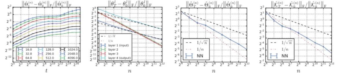
Figure 1: Relative Frobenius norm change during training. Three hidden layer ReLU net-works trained with ⌘ = 1.0 on a subset of MNIST (|D| = 128). We measure changes of (in-put/output/intermediary) weights, empirical⇥ˆ, and empiricalKˆ afterT = 217steps of gradient
descent updates for varying width. We see that the relative change in input/output weights scales as 1/pnwhile intermediate weights scales as1/n, this is because the dimension of the input/output does not grow withn. The change in⇥ˆ andKˆ is upper bounded byO(1/pn)but is closer to
O(1/n). See FigureS6for the same experiment with 3-layertanhand 1-layerReLUnetworks. See FiguresS9andS10for additional comparisons of finite width empirical and analytic kernels. from GD training does not generally correspond to a Bayesian posterior). We believe understand-ing the biases over learned functions induced by different trainunderstand-ing schemes and architectures is a fascinating avenue for future work.
2.4 Infinite width networks are linearized networks
Equation2and3of the original network are intractable in general, since⇥tˆ evolves with time. However, for the mean squared loss, we are able to prove formally that, as long as the learning rate ⌘<⌘critical:= 2( min(⇥) + max(⇥)) 1, where min/max(⇥)is the min/max eigenvalue of⇥, the gradient descent dynamics of the original neural network falls into its linearized dynamics regime. Theorem 2.1(Informal). Letn1 =· · · = nL =nand assume min(⇥)>0. Applying gradient
descent with learning rate⌘<⌘critical(or gradient flow), for everyx2Rn0withkxk21, with
probability arbitrarily close to 1 over random initialization,
sup t 0 ft(x) ftlin(x) 2, sup t 0 k✓t ✓0k2 pn , sup t 0 ˆ ⇥t ⇥ˆ0 F =O(n 1 2), as n! 1. (17)
Therefore, asn ! 1, the distributions offt(x)and ftlin(x)become the same. Coupling with
Corollary1, we have
Theorem 2.2. If⌘ <⌘critical, then for everyx2Rn0 withkxk21, asn! 1,ft(x)converges in distribution to the Gaussian with mean and variance given by Equation14and Equation15.
We refer the readers to Figure 2for empirical verification of this theorem. The proof of Theorem2.1 consists of two steps. The first step is to prove the global convergence of overparameterized neural networks [19,20,21,22] and stability of the NTK under gradient descent (and gradient flow); see SM §G. This stability was first observed and proved in [13] in the gradient flow and sequential limit (i.e. lettingn1! 1, . . . ,nL ! 1sequentially) setting under certain assumptions about global
convergence of gradient flow. In §G, we show how to use the NTK to provide a self-contained (and cleaner) proof of such global convergence and the stability of NTK simultaneously. The second step is to couple the stability of NTK with Grönwall’s type arguments [38] to upper bound the discrepancy betweenftandftlin, i.e. the first norm in Equation17. Intuitively, the ODE of the original network
(Equation3) can be considered as ak⇥tˆ ⇥ˆ0kF-fluctuation from the linearized ODE (Equation7).
One expects the difference between the solutions of these two ODEs to be upper bounded by some functional ofk⇥tˆ ⇥ˆ0kF; see SM §H. Therefore, for a large width network, the training dynamics
can be well approximated by linearized dynamics.
Note that the updates for individual weights in Equation6vanish in the infinite width limit, which for instance can be seen from the explicit width dependence of the gradients in the NTK parameterization. Individual weights move by a vanishingly small amount for wide networks in this regime of dynamics, as do hidden layer activations, but they collectively conspire to provide a finite change in the final output of the network, as is necessary for training. An additional insight gained from linearization
of the network is that the individual instance dynamics derived in [13] can be viewed as a random features method,11where the features are the gradients of the model with respect to its weights. 2.5 Extensions to other optimizers, architectures, and losses
Our theoretical analysis thus far has focused on fully-connected single-output architectures trained by full batch gradient descent. In SM §Bwe derive corresponding results for: networks with multi-dimensional outputs, training against a cross entropy loss, and gradient descent with momentum. In addition to these generalizations, there is good reason to suspect the results to extend to much broader class of models and optimization procedures. In particular, a wealth of recent literature suggests that the mean field theory governing the wide network limit of fully-connected models [32,
33] extends naturally to residual networks [35], CNNs [34], RNNs [39], batch normalization [40], and to broad architectures [37]. We postpone the development of these additional theoretical extensions in favor of an empirical investigation of linearization for a variety of architectures.
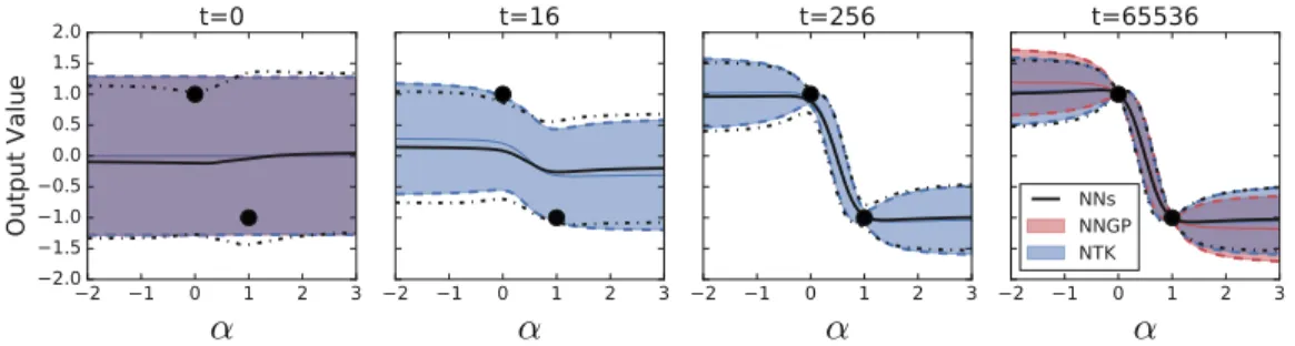
Figure 2: Dynamics of mean and variance of trained neural network outputs follow analytic dynamics from linearization. Black lines indicate the time evolution of the predictive output distribution from an ensemble of 100 trained neural networks (NNs). The blue region indicates the analytic prediction of the output distribution throughout training (Equations14,15). Finally, the red region indicates the prediction that would result from training only the top layer, corresponding to an NNGP (EquationsS22,S23). The trained network has 3 hidden layers of width 8192,tanhactivation functions, 2
w= 1.5, no bias, and⌘ = 0.5. The output is computed for inputs interpolated between
two training points (denoted with black dots)x(↵) =↵x(1)+ (1 ↵)x(2). The shaded region and
dotted lines denote 2 standard deviations (⇠95%quantile) from the mean denoted in solid lines. Training was performed with full-batch gradient descent with dataset size|D|= 128. For dynamics for individual function initializations, see SM FigureS1.
3 Experiments
In this section, we provide empirical support showing that the training dynamics of wide neural networks are well captured by linearized models. We consider fully-connected, convolutional, and wide ResNet architectures trained with full- and mini- batch gradient descent using learning rates sufficiently small so that the continuous time approximation holds well. We consider two-class classification on CIFAR-10 (horses and planes) as well as ten-class classification on MNIST and CIFAR-10. When using MSE loss, we treat the binary classification task as regression with one class regressing to+1and the other to 1.
Experiments in Figures1,4,S2,S3,S4,S5andS6, were done in JAX [41]. The remaining experi-ments used TensorFlow [42]. An open source implementation of this work providing tools to inves-tigate linearized learning dynamics is available atwww.github.com/google/neural-tangents [15].
Predictive output distribution: In the case of an MSE loss, the output distribution remains Gaussian throughout training. In Figure2, the predictive output distribution for input points interpolated between two training points is shown for an ensemble of neural networks and their corresponding GPs. The interpolation is given byx(↵) =↵x(1)+ (1 ↵)x(2)wherex(1,2)are two training inputs
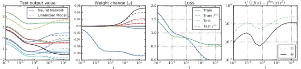
Figure 3: Full batch gradient descent on a model behaves similarly to analytic dynamics on its linearization, both for network outputs, and also for individual weights. A binary CIFAR classification task with MSE loss and aReLUfully-connected network with 5 hidden layers of width n= 2048,⌘= 0.01,|D|= 256,k= 1, 2
w= 2.0, and b2= 0.1. Left two panes show dynamics for
a randomly selected subset of datapoints or parameters. Third pane shows that the dynamics of loss for training and test points agree well between the original and linearized model. The last pane shows the dynamics of RMSE between the two models on test points. We observe that the empirical kernel
ˆ
⇥gives more accurate dynamics for finite width networks.
with different classes. We observe that the mean and variance dynamics of neural network outputs during gradient descent training follow the analytic dynamics from linearization well (Equations 14,15). Moreover the NNGP predictive distribution which corresponds to exact Bayesian inference, while similar, is noticeablydifferentfrom the predictive distribution at the end of gradient descent training. For dynamics for individual function draws see SM FigureS1.
Comparison of training dynamics of linearized network to original network: For a particular realization of a finite width network, one can analytically predict the dynamics of the weights and outputs over the course of training using the empirical tangent kernel at initialization. In Figures 3,4(see alsoS2,S3), we compare these linearized dynamics (Equations8,9) with the result of training the actual network. In all cases we see remarkably good agreement. We also observe that for finite networks, dynamics predicted using the empirical kernel⇥ˆ better match the data than those obtained using the infinite-width, analytic, kernel⇥. To understand this we note that k⇥ˆ(Tn) ⇥ˆ
(n)
0 kF =O(1/n)O(1/pn) =k⇥ˆ(0n) ⇥kF, where⇥ˆ(0n)denotes the empirical tangent
kernel of widthnnetwork, as plotted in Figure1.
One can directly optimize parameters offlininstead of solving the ODE induced by the tangent kernel⇥ˆ. Standard neural network optimization techniques such as mini-batching, weight decay, and data augmentation can be directly applied. In Figure4(S2,S3), we compared the training dynamics of the linearized and original network while directly training both networks.
With direct optimization of linearized model, we tested full (|D|= 50,000) MNIST digit classifica-tion with cross-entropy loss, and trained with a momentum optimizer (FigureS3). For cross-entropy loss with softmax output, some logits at late times grow indefinitely, in contrast to MSE loss where logits converge to target value. The error between original and linearized model for cross entropy loss becomes much worse at late times if the two models deviate significantly before the logits enter their late-time steady-growth regime (See FigureS4).
Linearized dynamics successfully describes the training of networks beyond vanilla fully-connected models. To demonstrate the generality of this procedure we show we can predict the learning dynamics of subclass of Wide Residual Networks (WRNs) [14]. WRNs are a class of model that are popular in computer vision and leverage convolutions, batch normalization, skip connections, and average pooling. In Figure4, we show a comparison between the linearized dynamics and the true dynamics for a wide residual network trained with MSE loss and SGD with momentum,trained on the full CIFAR-10 dataset. We slightly modified the block structure described in TableS1so that each layer has a constant number of channels (1024 in this case), and otherwise followed the original implementation. As elsewhere, we see strong agreement between the predicted dynamics and the result of training.
Effects of dataset size: The training dynamics of a neural network match those of its linearization when the width is infinite and the dataset is finite. In previous experiments, we chose sufficiently wide networks to achieve small error between neural networks and their linearization for smaller
Figure 4:A wide residual network and its linearization behave similarly when both are trained by SGD with momentum on MSE loss on CIFAR-10. We adopt the network architecture from Zagoruyko and Komodakis [14]. We useN = 1, channel size1024, ⌘ = 1.0, = 0.9, k= 10, 2
w = 1.0, and b2= 0.0. See TableS1for details of the architecture. Both the linearized
and original model are trained directly on full CIFAR-10 (|D|= 50,000), using SGD with batch size 8. Output dynamics for a randomly selected subset of train and test points are shown in the first two panes. Last two panes show training and accuracy curves for the original and linearized networks. datasets. Overall, we observe that as the width grows the error decreases (FigureS5). Additionally, we see that the error grows in the size of the dataset. Thus, although error grows with dataset this can be counterbalanced by a corresponding increase in the model size.
4 Discussion
We showed theoretically that the learning dynamics in parameter space of deep nonlinear neural networks are exactly described by a linearized model in the infinite width limit. Empirical investiga-tion revealed that this agrees well with actual training dynamics and predictive distribuinvestiga-tions across fully-connected, convolutional, and even wide residual network architectures, as well as with different optimizers (gradient descent, momentum, mini-batching) and loss functions (MSE, cross-entropy). Our results suggest that a surprising number of realistic neural networks may be operating in the regime we studied. This is further consistent with recent experimental work showing that neural networks are often robust to re-initialization but not re-randomization of layers (Zhang et al. [43]). In the regime we study, since the learning dynamics are fully captured by the kernel⇥ˆ and the target signal, studying the properties of⇥ˆ to determine trainability and generalization are interesting future directions. Furthermore, the infinite width limit gives us a simple characterization of both gradient descent and Bayesian inference. By studying properties of the NNGP kernelKand the tangent kernel
⇥, we may shed light on the inductive bias of gradient descent.
Some layers of modern neural networks may be operating far from the linearized regime. Preliminary observations in Lee et al. [5] showed that wide neural networks trained with SGD perform similarly to the corresponding GPs as width increase, while GPs still outperform trained neural networks for both small and large dataset size. Furthermore, in Novak et al. [7], it is shown that the comparison of performance between finite- and infinite-width networks is highly architecture-dependent. In particular, it was found that infinite-width networks perform as well as or better than their finite-width counterparts for many fully-connected or locally-connected architectures. However, the opposite was found in the case of convolutional networks without pooling. It is still an open research question to determine the main factors that determine these performance gaps. We believe that examining the behavior of infinitely wide networks provides a strong basis from which to build up a systematic understanding of finite-width networks (and/or networks trained with large learning rates).
Acknowledgements
We thank Greg Yang and Alex Alemi for useful discussions and feedback. We are grateful to Daniel Freeman, Alex Irpan and anonymous reviewers for providing valuable feedbacks on the draft. We thank the JAX team for developing a language which makes model linearization and NTK computation straightforward. We would like to especially thank Matthew Johnson for support and debugging help.
References
[1] Alex Krizhevsky, Ilya Sutskever, and Geoffrey E Hinton. Imagenet classification with deep convolutional neural networks. InAdvances in Neural Information Processing Systems. 2012. [2] Kaiming He, Xiangyu Zhang, Shaoqing Ren, and Jian Sun. Deep residual learning for image recognition. InConference on Computer Vision and Pattern Recognition, pages 770–778, 2016. [3] Jacob Devlin, Ming-Wei Chang, Kenton Lee, and Kristina Toutanova. Bert: Pre-training of
deep bidirectional transformers for language understanding.arXiv preprint arXiv:1810.04805, 2018.
[4] Radford M. Neal. Priors for infinite networks (tech. rep. no. crg-tr-94-1). University of Toronto, 1994.
[5] Jaehoon Lee, Yasaman Bahri, Roman Novak, Sam Schoenholz, Jeffrey Pennington, and Jascha Sohl-dickstein. Deep neural networks as gaussian processes. InInternational Conference on Learning Representations, 2018.
[6] Alexander G. de G. Matthews, Jiri Hron, Mark Rowland, Richard E. Turner, and Zoubin Ghahramani. Gaussian process behaviour in wide deep neural networks. In International Conference on Learning Representations, 4 2018. URLhttps://openreview.net/forum? id=H1-nGgWC-.
[7] Roman Novak, Lechao Xiao, Jaehoon Lee, Yasaman Bahri, Greg Yang, Jiri Hron, Daniel A. Abolafia, Jeffrey Pennington, and Jascha Sohl-Dickstein. Bayesian deep convolutional net-works with many channels are gaussian processes. InInternational Conference on Learning Representations, 2019.
[8] Adrià Garriga-Alonso, Laurence Aitchison, and Carl Edward Rasmussen. Deep convolutional networks as shallow gaussian processes. InInternational Conference on Learning Representa-tions, 2019.
[9] Behnam Neyshabur, Ryota Tomioka, and Nathan Srebro. In search of the real inductive bias: On the role of implicit regularization in deep learning. InInternational Conference on Learning Representations workshop track, 2015.
[10] Roman Novak, Yasaman Bahri, Daniel A. Abolafia, Jeffrey Pennington, and Jascha Sohl-Dickstein. Sensitivity and generalization in neural networks: an empirical study. InInternational Conference on Learning Representations, 2018.
[11] Behnam Neyshabur, Zhiyuan Li, Srinadh Bhojanapalli, Yann LeCun, and Nathan Srebro. The role of over-parametrization in generalization of neural networks. InInternational Conference on Learning Representations, 2019.
[12] Alexander G. de G. Matthews, Jiri Hron, Richard E. Turner, and Zoubin Ghahramani. Sample-then-optimize posterior sampling for bayesian linear models. InNeurIPS Workshop on Advances in Approximate Bayesian Inference, 2017. URL http://approximateinference.org/ 2017/accepted/MatthewsEtAl2017.pdf.
[13] Arthur Jacot, Franck Gabriel, and Clement Hongler. Neural tangent kernel: Convergence and generalization in neural networks. InAdvances in Neural Information Processing Systems, 2018.
[14] Sergey Zagoruyko and Nikos Komodakis. Wide residual networks. InBritish Machine Vision Conference, 2016.
[15] Roman Novak, Lechao Xiao, Jiri Hron, Jaehoon Lee, Jascha Sohl-Dickstein, and Samuel S. Schoenholz. Neural tangents: Fast and easy infinite neural networks in python, 2019. URL http://github.com/google/neural-tangents.
[16] Amit Daniely, Roy Frostig, and Yoram Singer. Toward deeper understanding of neural networks: The power of initialization and a dual view on expressivity. InAdvances In Neural Information Processing Systems, 2016.
[17] Amit Daniely. SGD learns the conjugate kernel class of the network. InAdvances in Neural Information Processing Systems, 2017.
[18] Andrew M Saxe, James L McClelland, and Surya Ganguli. Exact solutions to the nonlinear dynamics of learning in deep linear neural networks. InInternational Conference on Learning Representations, 2014.
[19] Simon S Du, Jason D Lee, Haochuan Li, Liwei Wang, and Xiyu Zhai. Gradient descent finds global minima of deep neural networks. InInternational Conference on Machine Learning, 2019.
[20] Zeyuan Allen-Zhu, Yuanzhi Li, and Zhao Song. A convergence theory for deep learning via over-parameterization. InInternational Conference on Machine Learning, 2019.
[21] Zeyuan Allen-Zhu, Yuanzhi Li, and Zhao Song. On the convergence rate of training recurrent neural networks. arXiv preprint arXiv:1810.12065, 2018.
[22] Difan Zou, Yuan Cao, Dongruo Zhou, and Quanquan Gu. Stochastic gradient descent optimizes over-parameterized deep relu networks. Machine Learning, 2019.
[23] Song Mei, Andrea Montanari, and Phan-Minh Nguyen. A mean field view of the landscape of two-layer neural networks. Proceedings of the National Academy of Sciences, 115(33): E7665–E7671, 2018.
[24] Lenaic Chizat and Francis Bach. On the global convergence of gradient descent for over-parameterized models using optimal transport. InAdvances in neural information processing systems, 2018.
[25] Grant M Rotskoff and Eric Vanden-Eijnden. Parameters as interacting particles: long time convergence and asymptotic error scaling of neural networks. InAdvances in neural information processing systems, 2018.
[26] Justin Sirignano and Konstantinos Spiliopoulos. Mean field analysis of neural networks.arXiv preprint arXiv:1805.01053, 2018.
[27] Xavier Glorot and Yoshua Bengio. Understanding the difficulty of training deep feedforward neural networks. InInternational Conference on Artificial Intelligence and Statistics, pages 249–256, 2010.
[28] Lenaic Chizat, Edouard Oyallon, and Francis Bach. On lazy training in differentiable program-ming. arXiv preprint arXiv:1812.07956, 2018.
[29] Twan van Laarhoven. L2 regularization versus batch and weight normalization.arXiv preprint arXiv:1706.05350, 2017.
[30] Tero Karras, Timo Aila, Samuli Laine, and Jaakko Lehtinen. Progressive growing of GANs for improved quality, stability, and variation. InInternational Conference on Learning Representa-tions, 2018.
[31] Daniel S. Park, Jascha Sohl-Dickstein, Quoc V. Le, and Samuel L. Smith. The effect of network width on stochastic gradient descent and generalization: an empirical study. InInternational Conference on Machine Learning, 2019.
[32] Ben Poole, Subhaneil Lahiri, Maithra Raghu, Jascha Sohl-Dickstein, and Surya Ganguli. Exponential expressivity in deep neural networks through transient chaos. InAdvances In Neural Information Processing Systems, pages 3360–3368, 2016.
[33] Samuel S Schoenholz, Justin Gilmer, Surya Ganguli, and Jascha Sohl-Dickstein. Deep informa-tion propagainforma-tion. International Conference on Learning Representations, 2017.
[34] Lechao Xiao, Yasaman Bahri, Jascha Sohl-Dickstein, Samuel Schoenholz, and Jeffrey Penning-ton. Dynamical isometry and a mean field theory of CNNs: How to train 10,000-layer vanilla convolutional neural networks. InInternational Conference on Machine Learning, 2018.
[35] Ge Yang and Samuel Schoenholz. Mean field residual networks: On the edge of chaos. In
Advances in Neural Information Processing Systems. 2017.
[36] Alexander G de G Matthews, Mark Rowland, Jiri Hron, Richard E Turner, and Zoubin Ghahramani. Gaussian process behaviour in wide deep neural networks. arXiv preprint arXiv:1804.11271, 9 2018.
[37] Greg Yang. Scaling limits of wide neural networks with weight sharing: Gaussian pro-cess behavior, gradient independence, and neural tangent kernel derivation. arXiv preprint arXiv:1902.04760, 2019.
[38] Sever Silvestru Dragomir. Some Gronwall type inequalities and applications. Nova Science Publishers New York, 2003.
[39] Minmin Chen, Jeffrey Pennington, and Samuel Schoenholz. Dynamical isometry and a mean field theory of RNNs: Gating enables signal propagation in recurrent neural networks. In
International Conference on Machine Learning, 2018.
[40] Greg Yang, Jeffrey Pennington, Vinay Rao, Jascha Sohl-Dickstein, and Samuel S. Schoen-holz. A mean field theory of batch normalization. InInternational Conference on Learning Representations, 2019.
[41] Roy Frostig, Peter Hawkins, Matthew Johnson, Chris Leary, and Dougal Maclaurin. JAX: Autograd and XLA.www.github.com/google/jax, 2018.
[42] Martín Abadi, Paul Barham, Jianmin Chen, Zhifeng Chen, Andy Davis, Jeffrey Dean, Matthieu Devin, Sanjay Ghemawat, Geoffrey Irving, Michael Isard, et al. Tensorflow: A system for large-scale machine learning. In12th USENIX Symposium on Operating Systems Design and Implementation (OSDI 16), 2016.
[43] Chiyuan Zhang, Samy Bengio, and Yoram Singer. Are all layers created equal? arXiv preprint arXiv:1902.01996, 2019.
[44] Ning Qian. On the momentum term in gradient descent learning algorithms.Neural networks, 12(1):145–151, 1999.
[45] Weijie Su, Stephen Boyd, and Emmanuel Candes. A differential equation for modeling nes-terov’s accelerated gradient method: Theory and insights. InAdvances in Neural Information Processing Systems, pages 2510–2518, 2014.
[46] Youngmin Cho and Lawrence K Saul. Kernel methods for deep learning. InAdvances in neural information processing systems, 2009.
[47] Christopher KI Williams. Computing with infinite networks. InAdvances in neural information processing systems, pages 295–301, 1997.
[48] Roman Vershynin. Introduction to the non-asymptotic analysis of random matrices. arXiv preprint arXiv:1011.3027, 2010.