Master Thesis in Finance Autumn 2009
An Application of the Hull-White Model
on CDS Spread Pricing
Supervisor: Anders Vilhemsson Author: Manshu Li
Abstract
This study illustrates in detail the Hull and White reduced-from model for pricing CDS spreads and applied the model to real bond data.
Following the assumption of the model, that the yield spread between a defaultable bond and a default-free bond only captures the probability of default, we aim at calculating a number of static CDS spread. To attain the CDS spread for different reference entities with time to maturity 1 to 5 years on May 15th, 2009, bond prices are carefully collected with special attention to
time to maturity and coupon payment. And then zero curves for both Treasury and corporate bonds are constructed using bootstrapping method and interpolation. Finally, theoretical default probabilities and CDS spread are calculated with recovery rate exogenously given as constant.
Our results shows it might be the reason that the model is based on a theoretical framework with rather strict assumptions, it is incapable of adjusting to situations where factors deviate from the given assumptions, that the yield spread only captures credit risk. Therefore the model does not perform ideally in practice.
Keywords: Yield spread, CDS spread, Credit default swap, Hull and White model.
1. INTRODUCTION...1
2. BACKGROUND...3
2.1.CREDIT DEFAULT SWAPS...3
2.2.TERM STRUCTURE...7
2.3.CREDIT PRICING MODELS...8
3. THE HULL AND WHITE MODEL...10
3.1.ESTIMATING DEFAULT PROBABILITIES AT DISCRETE TIMES...10
3.2.THE MODEL’S PRECONDITION...14
4. APPLICATION OF THE MODEL...15
4.1.SIMPLIFIED ASSUMPTIONS...15
4.2.DATA...16
4.3.VALUATION OF THE CDS SPREAD...17
4.3.1. Treasury Zero Curve...20
4.3.2 Corporate Zero Curve...23
4.3.3. Default Probabilities and CDS spread...24
4.3.4. Theoretical CDS spread and Quoted CDS spread...31
5. ANALYSIS...34
5.1.INTERPRETATION OF THE RESULTS...34
5.2.ANALYSIS OF PRICING ERROR...35
6. CONCLUSION...38
REFERENCES...39
APPENDIX 1. COMPANIES INCLUDED IN THE STUDY...41
APPENDIX 2. EMPIRICAL FINDINGS ON RECOVERY RATE...42
1. Introduction
Most financial assets are, in one way or another, subject to credit risk: the uncertainty surrounding the counterparty’s ability to meet its financial obligations. The three main variables that affect the credit risk of a financial asset are: (i) default probability, (ii) loss given default, which equals to one minus recovery rate in the event of default, and (iii) the exposure at default. Credit risk can be dealt with by transferring the underlying asset or by using credit derivatives. Credit default swaps (CDS) are in the most widespread use among various credit derivatives.
Credit risk has become a topical issue in the awake of the recent credit crisis. And the massive CDS market has been believed to exacerbate the global financial meltdown starting in 2008. “Credit default swaps have played a prominent role in the mushrooming credit crisis that in the past month led to Lehman filing for bankruptcy protection, a government rescue plan for insurer American International Group Inc. and Merrill Lynch & Co. selling itself to Bank of America Corp.” (International Business Times, 2009) Therefore it is reasonable to question whether credit risk transferring is a stabilizing mechanism or more of concentration. As many other financial derivatives, CDS can be used as an instrument for hedging, arbitraging and speculating. Speculating and arbitraging exist only when investors think the CDS spread is higher or lower than its fair price therefore the importance of accurate pricing must be drawn to prevent the massive use of CDS, which exacerbate the financial crisis. This is quite a big issue to discuss with different perspectives and dimensions. However, we believe that if the CDS spreads are correctly priced then no arbitrage opportunities can be found in the market as a whole, CDS can be served mainly as a good instrument to transfer credit risk. Hence we think pricing factors and pricing techniques are vital in credit derivatives, in particular the CDS market.
Combining our interests in the extensive credit world together with our academic background, what we think is a doable project for this thesis is to look deeply into a particular credit model, which can be used to price CDS spread. We choose the no-arbitrage reduced-form model proposed by Hull and White (2000). Our goal is to apply the Hull and White model to real bond data with some simplified assumptions and calculate the corresponding CDS spread. By comparing the theoretical CDS spread with the CDS spread quoted on the market, we can criticize on how well the model works, which assumptions in the modeling framework should be released and if there might be any additional pricing factors which are omitted in the original modeling framework. By concluding we hope we will be able to give some suggestions on better projections of the credit risk modeling process and a more accurate pricing technique of the CDS spread.
The main objective in this paper is to explain and illustrate how Hull-White has constructed and developed a model for the pricing of CDS spread and to apply the model to real bond data on the market. Furthermore we will compare the CDS spread calculated using Hull and White model with the quoted spread from the market. The questions we will try to address are hence how effective the Hull-White model is when it is applied on real data and if there is a possibility to substitute bits and pieces originally used in the equation for more accurate results. Due to the restrictions in time we limit our research to cover only the very first of Hull and White paper where the modeling is done in discrete time framework. Although we urge the interested readers to cover all of the articles covered to a more extensive modeling technique.
The rest of the paper is organized as follows. Section 2 presents the theoretical and empirical background in this field, with an in-depth introduction on CDS and two main classes of credit pricing models. Section 3 presents the Hull and
White reduced-form model. Section 4 provides how we apply the model in this paper and the theoretical results. The analysis of pricing errors and interpretation of our empirical results are provided in Section 5 and Section 6 concludes.
2. Background
2.1. Credit Default Swaps
This section is mainly in place to give the reader a broader understanding around how this derivative is constructed and to what purpose it has for the buyer vis-à-vis seller. Since this paper is written around this specific derivative it is important to give a thorough description of it before we go any further. In order to simplify for the readers we have chosen to use the same terminology as Hull and White when it comes to describing credit derivatives and the CDS in particular.
O´Kane and Turnbull (2003) described the CDS and gave an explanation for the rapid growth of this specific derivative. The reason was and still is the unique possibility for agents to hedge or speculate in the credit worthiness of a company without taking an opposite position.
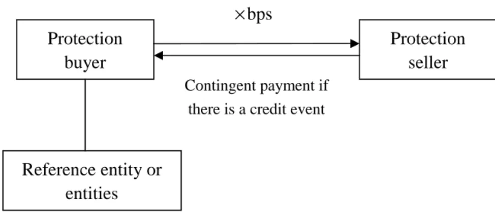
The CDS is a contract entered between two parties, where the protection buyer pays a fee or a premium to the protection seller in order to acquire insurance against a credit event by a third party, i.e. the reference entity. This fee is measured in basic point (bps), which is one hundredth of a percentage point (0.01%) and is in most cases paid over the lifespan of the contract in form of regular payments. Hence the payment structure consists of payments from the protection buyer until the end of the contract or a credit event occurs. In case of a credit event, the payments come to an end and the protection seller will fulfill the contract by compensating the protection buyer with a
sum that reflects the face value the bond would have had in the absence of a credit event (O’Kane, Turnbull (2003)).
Figure 1. Mechanics of a Credit Default Swap
The reference entity is most commonly embodied as a bank, a corporate or a sovereign issuer and the legal jurisdictions can differ among the three. The CDS is designed to be triggered when the reference entity defaults, fails to pay up, is restructured or when any other credit event occurs. The contract itself could be tailor-made in order to suit the protection buyer or seller but the contracts are in fact most often standardized to increase the ability to sell and to simplify the trading procedure. The typical contract is over five years but might as well run over three, seven or any other number of years. If a credit event occurs and the reference entity fails to deliver its payments the contract stipulates that there will be a settlement between the protected buyer and the protected seller. This settlement will be reached either as a cash settlement or as a physical settlement. If there would to be a physical settlement the protection seller will pay a pre-determined amount (usually equals to the face value of the debt) and in exchange overtake the remaining value of the debt, a value which usually is significantly smaller than the face value of the debt after a credit event. The term “physical” is referring to the fact that the bond is physically delivered to the protection seller in exchange
Protection buyer Protection seller Reference entity or entities Contingent payment if there is a credit event
for cash. If the contract stipulates a cash-settlement, the protection seller will have to deliver the cash difference between the remaining value of the debt and what would have been its face value. The remaining value of the defaulted bond is often determined a couple of weeks after the credit event has taken place by a dealer poll (O’Kane, Turnbull (2003)).
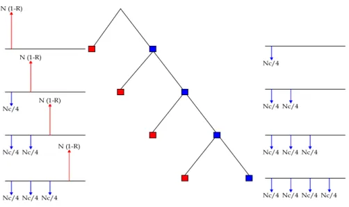
N (1-R) N (1-R) Nc/4 Nc/4 Nc/4 Nc/4 Nc/4 Nc/4 Nc/4 Nc/4 Nc/4 Nc/4 Nc/4 Nc/4 Nc/4 Nc/4 Nc/4 Nc/4 N (1-R) N (1-R)
Figure 2. Payoff of a CDS contract
We now give a simple example of how CDS works. Assume a bond, which has the face value of $5 million and the yearly credit spread is measured at 400bps. In case of payment structure that stipulates semi-annual payments, the protection buyer will pay a fee that equals 0.04 0.5 $5 million = $100000. This means that the protection buyer pays a fee of $100000 every six months until the end of the contract or until a credit event which ever happens first. Now lets assume that if a credit event occurs and the insured asset will have a value equals $35 per $100 of the face value the following payments will look as followed. The protection seller compensates the buyer with the difference
between the face value and the current value of the asset. This in term measures as $5 million ($100 - $35) = $ 3.25 million.
The protection buyer fulfills the contract by paying the remaining accrued interest that counts from the date of the latest down payment. That could equal for example 0.04 * 2/12 *5 million = 200000 if the last payment occurred two months ago (O’Kane, Turnbull (2003)).
What is examined in this paper will mainly be one approach to how this spread that determines the fee is valued. And try to analyze how the results correspond to the markets valuation.
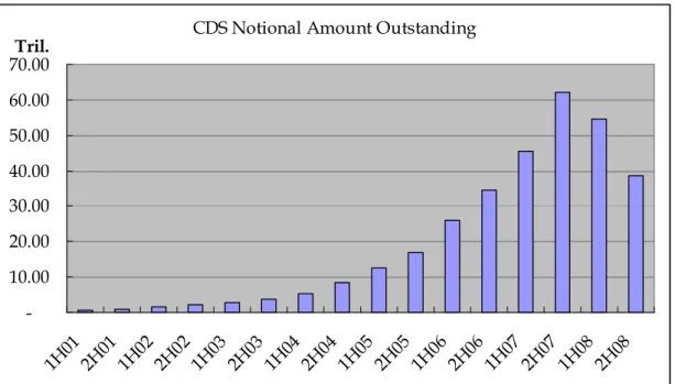
As mentioned before, CDS is among the most widely used credit derivatives, representing over thirty percent of the credit derivatives market. Although the form of CDS had been in existence from at least the early 1990s, the modern CDS were invented in 1997 and initially for banks to transfer the risk of default on their loans to the third party. However, as the market matured, CDS became to be used less by banks seeking to hedge against default and more by investors wishing to bet for or against the likelihood that particular companies or portfolios would suffer financial difficulties, as well as those seeking to profit from perceived mispricing. The market size for CDS began to grow rapidly from 2003, and by the end of 2007, the CDS market had a notional value of $45 trillion. But notional amount began to fall during 2008 and by the end of 2008 notional amount outstanding had fallen 38 percent to $38.6 trillion. (ISDA Market Survey) However, it is important to note that since default is a relatively rare occurrence and in most CDS contracts the only payments are the spread payments from buyer to seller. Thus, although the notional amount of the outstanding CDS contracts sounds very large, the net cash flows are generally only a small fraction of this total.
It is worth noticing that after 2005, the notional amount of the outstanding CDS contracts started to surpass the total amount of the bank and non-bank loan plus corporate and foreign bonds and in 2007, the former is four times big as the latter. This, we think, implies the excessive use of CDS as a preferable instrument for speculating and arbitraging. And again, it draws the attention of the possible mispricing of CDS spread. (ISDA Market Survey, FED)
CDS Notional Amount Outstanding
-10.00 20.00 30.00 40.00 50.00 60.00 70.00 1H01 2H01 1H02 2H02 1H03 2H03 1H04 2H04 1H05 2H05 1H06 2H06 1H07 2H07 1H08 2H08 Tril.
Figure 3. Notional amount of outstanding CDS contract
2.2. Term Structure
The term structure or the yield curve as it is usually referred to explains the relationship between the interest rate and time to maturity. The term yield curve could take different shapes and could hence be upwards sloping, downwards sloping or humped shaped. In economic theory it is most common to assume an increasing term structure, i.e. an upward-sloping yield curve. The reasoning behind this includes assumptions about interest rate risk where investors want compensation for tying down an investment. The assumptions around the term-structure are central in the buildup of the Hull
and White (2000) model and will be discussed in detail later on. (Options, Futures and Other Derivatives, Hull 2005)
2.3. Credit Pricing Models
Credit pricing models can be divided into two main categories: structural-form models and reduced-form models. Structural models are based on the original framework developed by Merton (1974) using the principles of Black and Scholes option pricing where the risk of a firm’s default is linked to the variability of the firm’s asset value. The intuition behind the Merton model is: default occurs when the value of a firm’s assets, i.e. the market value of the firm, is lower than that of its liabilities. Therefore the payment to the debtholders at maturity is the smaller than the face value of the debt or the market value of the firm’s assets. Assuming the firm’s debt is entirely represented by a zero-coupon bond, at maturity, if the value of the firm is larger than the face value of the bond, then the bondholder gets back the face value of the bond; if the value of the firm is smaller than the face value of the bond, default occurs and the bondholders get the market value of the firm. Therefore, the payoff at maturity to the bondholder is the face value of the bond minus a put option on the value of the firm’s assets, with the exercising price equal to the face value of the bond and a maturity equals to the bond’s maturity, i.e. payoff = F-min[0, V-F]. Following this basic intuition, Merton developed an explicit formula for risky bonds which can be used to estimate both the default probability of a firm and the credit spread between a risky bond and a default-free bond.
Structural-form model has certain advantages: they use market prices; they have a forward perspective rather than a historical one and they consider the credit events not unpredictable, i.e. default is an endogenous factor.
However, some assumptions of Merton’s framework are unrealistic. Black and Cox (1976) released the assumption of no seniority difference among bonds issued by the same firm by introducing the possibility of more complex capital structures, with subordinated debt; Geske (1977) introduced coupon-paying bond; Vasicek (1984) introduced the distinction between short and long term liabilities. There are a set of models under Merton’s framework but remove the assumption that default can only happen at maturity when the firm’s assets value are no longer to cover the debt obligation, including Kim, Ramaswamy and Sundaresan (1993), Hull and White (1995), Longstaff and Schwartz (1995) among others. These models introduce a default barrier where credit event may occur anytime between the issuance and maturity when the value of the firm’s assets hits the default barrier. However, for all structural-form models, the biggest problem is that the firm’s assets value is most commonly not observable which makes these models difficult to implement in practice.
Reduced-form models are introduced with the aim of overcoming the shortcomings of structural-form models. These models include Litterman and Iben (1991), Jarrow and Turnbull (1995), Jarrow, Lando and Turnbull (1997), Lando (1998), Duffie and Singleton (1999), Duffie (1999). The model we are examining in this paper, Hull and White (2000) is also included in this set. Reduced-form models do not condition default on the value of the firm’s assets hence parameters related to the firm’s assets value need not be estimated to implement the model. Noticeably, although all these models have the objective of obtaining the spread of risky bond rates over default-free bond rates, under the non-arbitrage assumption, considerable differences can be found among different reduced-form approaches due to the different input information required and different specification on the event of default and recovery rate.
Comparing these two classes of models, we can see the fundamental hypothesis of structural-form models is that the modeler has continuous information on the firm’s assets value, which in many cases result in the prediction of the firm’s default while in reduced-form models the information required is less refined, which is the reason for the fact that default time is seen as unpredictable. However, Jarrow et al (2004) shows that “these models are not disconnected and disjoint models types as is commonly supposed, but rather they are really the same model containing different informational assumptions”, “Indeed, structural models can be transformed into reduced form models as the information set changes and becomes less refined, from that observable by the firm’s management to that which is observed by the market.”
Since our goal is to price CDS spread, and the firm’s assets value process is unobservable by the market, we will apply Hull and White (2000) among the reduced-form models.
3. The Hull and White Model
3.1. Estimating Default Probabilities at Discrete Times
In order to present the Hull and White (2000) model it’s convenient to define the different parameters variables used. Beneath, are the components used for the formula of calculating risk-neutral probabilities.
j
B : Price of thejth bond today
j
G : Price of the jth bond today if there were no probability of default
) (t
Fj : Forward price of the jth bond for a forward contract maturing at time
) (t
Cj : Claim made by holders of thejth bond if there is a default at time t, (t <tj)
) (t
v : Present value of $1 received at time t with certainty
) (t
Rj : Recovery rate for holders of the jth bond in the event of a default at time t, (t <tj)
ij
α : Present value of the loss, relative to the value of the bond would have if there were no possibility of default, from a default on the jth bond at time ti
i
p : The risk-neutral probability of default at time ti
In this model, Hull and White use the Treasury bond as a proxy of default-free bond hence Gj is the price of a Treasury bond promising the same cash flows as the jth defaultable bond and the valuation of the CDS spread is determined by the fact that default only occurs at the reference entity and that no counterparty default risk is present. Hence the model only takes into account that the reference entity could default and not the protection seller. The Hull and White model is based on the assumptions that are used in most cases with the reduced-form model framework and presumes that interest rates, default probabilities and recovery rates are independent and exogenously given. The model can then be tested on its sensitivity to different factors like claim amount by bondholders and recovery rate.
The first step to retrieve any results is to acquire risk-neutral default probabilities, as they are the key elements in the final equation of calculating CDS spread. In order to attain these default probabilities we need to make an
assumption on yield spreads, which is that, the difference between a defaultable bond yield and a default-free bond yield only captures the risk of default. With this assumption taken into account, we can extract the price of default in the difference in yield between the two bonds. We can construct yield curves out of bonds issued by a reference entity and with a comparison to the curve constructed by the default-free bonds we get default probabilities at different times to maturity. Since Hull and White (2000) are using the treasury rate as the proxy for the default-free bond, we need a corporate yield curve, a treasury curve and an assumption about recovery rate to get a simple estimate.
Let us take a very simplifying example of how this risk-neutral probability is calculated and we will then show how it was done in our study. If we for example have a default-free and a defaultable bond that both matures in five years and the zero coupon return rate is 3% and 4% respectively. If both bonds have a face value of $100 the cost of default in a risk neutral world would be 1977 . 4 ) 100 ( ) 100 ( e−0.04×5 − e−0.03×5 =
With the value of the default we can now incorporate the risk neutral default probability, which is defined as pj. With the information above and the assumption and no recovery rate it gives that
1977 . 4 100pe−0.03×5 =
which gives a value on p= 4.3%. This way of retrieving risk-neutral default probabilities is central in the build-up of the model. And an issue of important notice is that the example above does not take into account the fact that the
recovery rate of a bond is in most cases not zero as described above and the corporate bond is rarely found to be a zero coupon bond.
With a non-zero recovery rate the equation looks a bit different. In addition to the recovery rate we also need to make an assumption about the claim of the bondholders. Hull and White (2000) argue that the most applicable assumption probably is the face value of the defaultable bon plus the accrued interest. Given these assumptions we can now get an equation that gives us the payoff for a CDS.
L - RL[1 + A(t)] = L[1 – R - A(t)] (1) Where L equals the face value, R is the recovery rate and A(t) is the accrued interest at the time of default. If we extend this analysis to a set where we have a number of bonds, N, given by a reference entity. The various bonds should have different times to maturity and default if this case can happen at any of the maturity dates of the bonds. The maturity of the ith bond with the condition that t1 < t2 < t3… < tN
To apply this in a discrete time framework as we are using through out this paper we need a situation where we collect a number of bonds from the same firm issued at the same date. These bonds should have different dates to maturity and also be within the same seniority i.e. the bonds have the same structural body in case of a default. The model now enables us to get a default probability at any of the different maturity dates of the bonds that the reference entity has issued given the assumption that a credit event actually can happen at any of these occasions.
If the claim and the recovery rates are observed and known in advance we can get something that looks like equation (2). Given that the bondholder
make a claim equal to Cj(ti) and given that we have a present value of the loss that equals to αij it is possible to get the following.
)] ( ) ( ) ( )[ (i j i j i j i ij =v t F t −R t C t α (2) Addressing the problem in similar fashion as in the very first and simple example where we had no recovery we can obtain the incurred probability of the loss. This we can get using a formula for the total value of all the losses from all the bonds used.
(3)
Well with this expression in hand we can use this to solve for the probabilities inductively.
(
1)
1 j j j i j ij j jj G B p pα
α
− = − − =∑
(4)With equation (4) we now have a formula that allows us to extract the risk-neutral probabilities of default from observed bond prices.
Given these results the first step to calculating a CDS-premium is accomplished. Hull and White (2000), advances with further extensions testing the models sensitivity for recovery rate, allowing default to happen at any time and investigations regarding the claim amount. Since those extensions are irrelevant to the discrete-time framework we will not go in to greater detail about that.
3.2. The Model’s precondition
In the way the model is constructed certain preconditions have to be satisfied in order to validate the model. For one thing the probability function from equation (4) must be greater that zero. This gives that
1
j j j i j ij G −B −
∑
= pα
∑
− − − ≤ 1 1 j i j ij j j G p Bα
(5)The second fundamental condition that must be satisfied for the model to give satisfactory results is that the cumulative probability needs to be less than one, which gives following expression.
) ( 1 ) ( 1 1 1 1
∑
− = − − ≤ − − − j i i i i j j j t t p t t p (6)this enables us to use equation (4) to get following results
− − − − − ≥
∑
∑
− = − − − = 1 1 1 1 1 1 ) ( 1 j i i i i j j jj ij j i i j j p t t t t p G Bα
α
(7)The equations above suggest that there is a boundary where the yield can move within. Once the recovery rate is set, equation (6) and (7) can be used to validate if the bond yields are applicable on the chosen recovery rate. If there are any discrepancies we have reason to believe that either the recovery rate assumption is out of fit or we have mispriced bonds.
4. Application of the model 4.1. Simplified assumptions
The model that will be more thoroughly examined in this thesis is the early and simplified version of the Hull and White (2000) with a discrete time framework. The reasoning behind the choice of the model is based on a few factors. One main advantage of using the simpler version is the fact that it has a pedagogical value and contributes with an easy insight to how a reduced- form model is constructed. The downside, however, is the probable loss of accuracy due to the fact that some values and calculations might suffer a bit in their estimations due to lack of scrutiny in the mathematical part. Our hope
nevertheless is that this simple version still captures the explanatory features of the reduced-form model sufficiently and gives an insightful guidance of how the different features and mechanisms are constructed. More advanced structure of the reduced-form models requires a substantial addition of complex and complicated mathematical features and would on this level of studies shift the focus to technicalities instead of capturing the core essence behind them.
To point out the differences between the Hull and White model and how it is implemented in this paper, it is important to stress that this paper only limits the analysis to discrete time framework. The major difference between a credit risk model in a discrete time framework and continuous time framework is that in discrete timeframe, default can only happen at maturity whereas in continuous timeframe, default can also happen anytime before maturity. With this known, it is easy to see that the concept of accrued interests is redundant in our application, i.e. A(t)=0. As for the assumption on the amount claim by the debtholders at the event of default, we adopt the Hull and White assumption of the claim equals the face value of the debt plus accrued interests and as explained above, accrued interests always equals to zero in our application hence the claim, C(t), always equals to the face value of the debt.
4.2. Data
The choice of data in this study is limited to only incorporate U.S. based companies. The reason behind this is associated with the fact that we use US-Treasuries as proxy for the default-free bond. Apart from the regional choice limitations in data availability restricts the possibility to choose freely among US companies.
With the date 15th of May, 2009 used as a standing point, we collected
information about zero-coupon Treasuries with time to maturity of three months, six months and one year. In addition to that coupon-paying US-Treasuries that matured in 1.5 years, 2 years,…,5 years. Same shall be implemented on corporate bonds, however a majority of the corporate zero-coupon bonds have very peculiar price, which made them unfit to use as inputs in the model. For example a corporate zero-coupon bond with three months to maturity was 1.5 times its face value. As a result, we collected only the prices of coupon-paying corporate bonds with different time to maturities. Further limitations of choice is handed by the fact that corporate bonds need to be interpolated in order to acquire the zero-rate curve. This limits the choice to companies with a numbers of outstanding bonds maturing between one and five years and reduces our sample to 20 companies. The chosen bonds in the sample are all senior bonds with semi-annual coupon payments, in order to maximize the coherence between the chosen samples.
The CDS data is collected through both Datastream and Reuters although there is only minor difference between the CDS quotes from these two databases. We collected CDS quote for only senior bonds, maturity 1 to 5 years. For simplicity all CDS spread data are mid quote data which is an average value of the bid and ask quotes.
4.3. Valuation of the CDS spread
For the valuation of the plain vanilla CDS a couple of additional parameters other than default probability need to be added in order to reach the final result. Previous assumptions are still need to be held, which means that recovery rates, default events and interest rates are all independent and that defaults can happen at any maturity date.
T: Life of credit default swap
) (t
p : Risk-neutral default probability at time t
R: Expected recovery rate of a reference entity in a risk neutral world. The recovery rate is expected to be independent of time; hence it takes on the same value regardless at what time a default occurs.
) (t
u : Present value of payments at the rate of $1 per year on payment dates between time zero and time t.
) (t
e : Present value of an accrual payment at time t equal to t-t* where t* is the payment date immediately preceding time t.
) (t
v : Present value of $1 received at time t.
w: Total payments per year made by credit default swap buyer
s: Value of w that causes the credit default swap to have a value of zero.
π
: The risk neutral probability of no credit event during the life of the swap.) (t
A : Accrued interest of the reference obligation at time t as a percent of face value.
The above presented probability of no default occurring can be written as and could be calculated from p(t).
∑
= − = T t t p 1 ) ( 1 π (8)Another new parameter that is introduced now is the payments w, and they will last until there is a credit event occurs or to the end of the CDS contract, which of them ever happens first. Should a default occur at time t (t<T) the present value of the payments made by the protection buyer is w[u(t) + e(t)]. Should no default occur the present value of the payments is simply wu(t). With this given the expected present value of the payments is given by the equation below.
[
]
∑
= + + T t T u w t e t u t p 1 ) ( ) ( ) ( ) ( π (9) Using the same assumption as we had in equation (1) we get the risk-neutral expected payoff from a CDS that looks like[
]
_ _ _ ) ( 1 ) ( 1 1− +A t R= −R−At R (10)The present value of the expected payoff given from the CDS then becomes
∑
= − − T t t v t p R t A R 1 _ _ ) ( ) ( ) ( 1 (11) To the buyer the value of a CDS is naturally the expected payoff in a case of a default minus the payments that is already made.[
( ) ( )]
( ) ) ( ) ( ) ( ) ( 1 _ _ T wu t e t u T wp t v t p R t A R = + −π − − (12) The CDS spread is then the value of w that makes the expression above equals to zero. The equation for the CDS spread can then be derived as shown below.[
( ) ( )]
( ) ) ( ) ( ) ( ) ( 1 1 _ _ T u t e t u t p t v t p R t A R s T t π + + − − =∑
= (13) The equation above gives us the total payments over a year expressed in percentage of the face value for a recently issued CDS. This equation now enables us to use the data collected to calculate the default probabilities and therefore the CDS spread presented in percentage. The spread is expressed annually, which coheres with the way the default probabilities are calculated. If a plain non-arbitrage reasoning is used it is possible to determinate the CDS spread, s, with this simple reasoning. If we have a situation where an investor holds a long position on a defaultable bond over T years and the equivalent CDS respectively the investor would be insured against most of the risk associated with the investment. The net return on this investment would then be y−s given that y is the annual yield of the bond and s is the spread. Without an arbitrage opportunity this investment should equal to the proxy of the risk free alternative i.e. the Treasury bond denoted as x. If that reasoning wouldn’t hold an arbitrageur would find an opportunity to benefit from the difference. Given this reasoning y−x should equal the CDS spread.4.3.1. Treasury Zero Curve
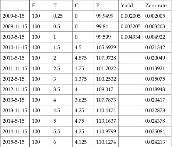
To get the zero curve for U.S. Treasury bond, we use the bootstrap method. Standing on May 15, 2009, it is possible to find U.S. Treasury bonds mature in exact 3 months, 6 months, 1 year, 1.5 years,…, up to 5 years. In order to bootstrap the zero curve, we find zero-coupon Treasury bond for time to maturity 3 months, 6 months and 1 year and semi-annual coupon paying Treasury bonds for time to maturity onwards till 5 years. Because the first three bonds pay no coupons, the zero rates corresponding to the maturites of
these bonds can easily be calculated. The 3-month bond provides a return of 0.0501 in 3 months on an initial investment of 99.9499. With quarterly compounding, the 3-month zero rate is (4×0.0501)/99.9499=0.2005% per annum. When the rate is expressed with continuous compounding, it becomes 002005 . 0 ) 4 002005 . 0 1 ln( 4 + =
or 0.2005% per annum. The 6-month bond provides a return of 0.16 in 6 months on an initial investment of 99.84. With semi-annual compounding the 6-month rate is (2×0.16)/99.84=0.3205% per annum. When the rate is expressed with continuous compounding, it becomes
003203 . 0 ) 2 003205 . 0 1 ln( 2 + =
or 0.3203% per annum. Similarly, the 1-year rate with continuous compounding is 004922 . 0 ) 509 . 99 491 . 0 1 ln( + = or 0.4922% per annum.
The forth bond lasts 1.5 years. The payments are as follows: 6 months: $2.25
1 year: $2.25 1.5 years: $102.25
From our earlier calculation, we know that the discount rate for the payment at the end of 6 months is 0.3203% and that the discount rate for the payment at the end of 1 year is 0.4922%. We also know that the bond’s price, $105.6929,
must equal the present value of all the payments received by the bondholder. Suppose the 1.5-year zero rate is denoted by R. It follows that
6929 . 105 25 . 102 25 . 2 25 . 2 e−0,003203×0.5 + e−0004922×1.0 + e−R×1.5 =
Using Goal Seeking function in Excel, we easily get R=0.021342. The 1.5-year zero rate is therefore 2.1342%.
Similarly, we calculated the 2-year, 2.5-year,…, up to 5-year zero rates and they are summarized in Table 1.
F T C P Yield Zero rate
2009-8-15 100 0.25 0 99.9499 0.002005 0.002005 2009-11-15 100 0.5 0 99.84 0.003205 0.003203 2010-5-15 100 1 0 99.509 0.004934 0.004922 2010-11-15 100 1.5 4.5 105.6929 0.021342 2011-5-15 100 2 4.875 107.9728 0.020049 2011-11-15 100 2.5 1.75 101.7022 0.013921 2012-5-15 100 3 1.375 100.2532 0.015075 2012-11-15 100 3.5 4 109.017 0.018943 2013-5-15 100 4 3.625 107.7873 0.020417 2013-11-15 100 4.5 4.25 110.4174 0.022878 2014-5-15 100 5 4.75 113.1637 0.024378 2014-11-15 100 5.5 4.25 110.9799 0.025084 2015-5-15 100 6 4.125 110.1274 0.024213
Table 1. Bootstrapped U.S. Treasury Zero Rates (*F: Face value of the bond. T: Time to
maturity. C: Coupon payment (all coupons are paid semi-annually). P: bond price. )
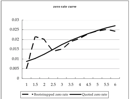
We also find the U.S zero curve from Datastream and we compare it with our bootstrapped zero curve.
zero rate curve 0 0.005 0.01 0.015 0.02 0.025 0.03 1 1.5 2 2.5 3 3.5 4 4.5 5 5.5 6 Bootstrapped zero rate Quoted zero rate
Figure 4. Bootstrapped Zero Rate and Quoted Zero Rate
From the figure above we can see that our bootstrapped zero curve goes closer to the Datastream zero curve as time to maturity increases. However, with shorter time to maturity, the difference is quite significant. As model input, however, we think it is more appropriate to use the quoted U.S. zero rate rather than bootstrapped zero rates. The reason is that the bond prices we used for the bootstrapping method contains other information than credit risk and the actual curve is more likely a smooth upward-sloping curve.
4.3.2 Corporate Zero Curve
To address the fact that most of the corporate bonds used in the sample had coupons we need to discount back the values of the coupons in order to get a zero curve. This is necessary in order to have a curve that is comparable to the Treasury curve used. The formula used to discount the cash-flows from the coupons is shown below.
t r C PV ) 1 ( + = (14)
where r is a feature of the economy, hence the equivalent Treasury rate. Should there be more than one coupon the equation can be written as
∑
= + = N i t i i r C PV 1 (1 )but since we can not use the same r for different t we need to use a formula where r changes with t
∑
= + = N i t i i i t z C PV 1 (1 ( ))Let us assume we have an example where a coupon-paying bond has three payment dates and a final payment. The coupon size is $6 and the final payment is $106, if the relevant interests are 6.611, 6.786, 6.982 and 7.190 respectively the discounted values will be: 5.811, 5.619, 5.422, 92.257. The present value then sums to 109.11, which gives a zero-yield of 9.11%.
This procedure is then repeated for all the bonds in the sample respectively to get the yield used for calculating the risk-neutral probabilities of default. After calculating a several zero-rates along the time line, linear interpolation was needed on corporate yields in order to attain the zero-rates for the preferred dates. To come around this problem, two corporate bonds are chosen. One that matures as close prior to the Treasury and another one that matures as close subsequently as possible. From these two bonds a linear interpolation is made to find a new bond price that matches the given date of the Treasury. With the interpolated result there is a possibility to compare the yield of the Treasury with to corporate on and out of that get a measurement of the probability that’s sought after.
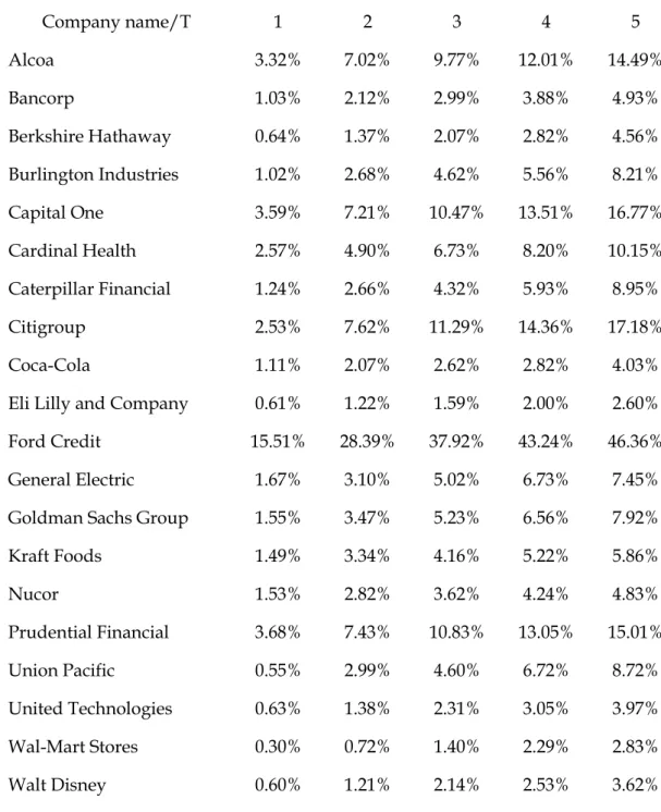
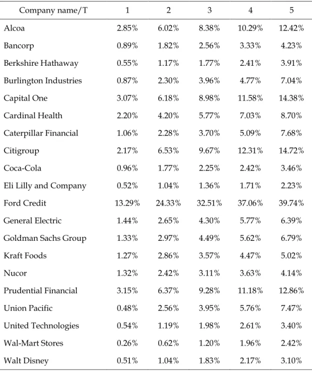
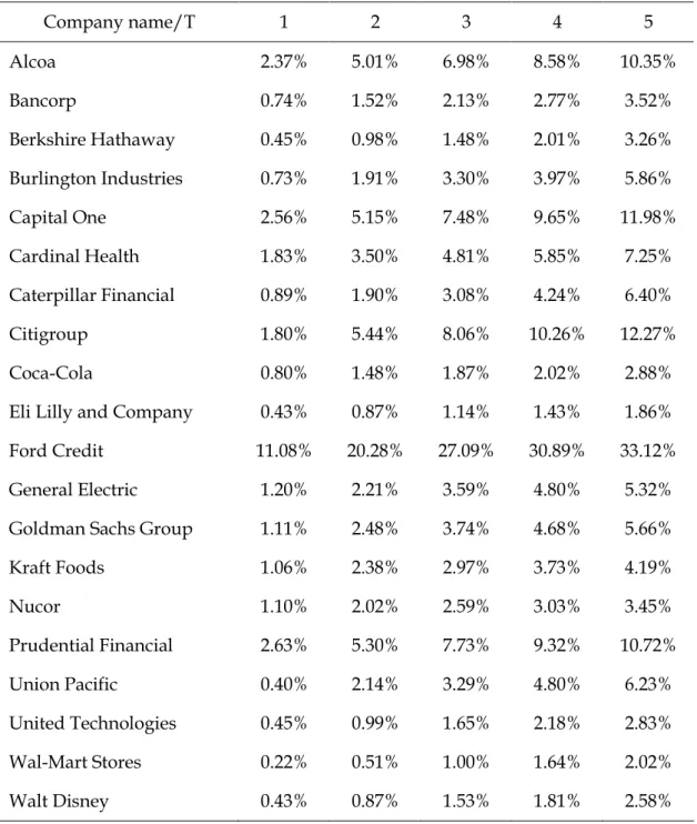
With the attained zero rates, we are now able to calculate the default probabilities and further CDS spread with different time to maturities for each company in sample with different assumptions on recovery rate. All calculations are done in Excel and the results are presented below.
Company name/T 1 2 3 4 5 Alcoa 3.32% 7.02% 9.77% 12.01% 14.49% Bancorp 1.03% 2.12% 2.99% 3.88% 4.93% Berkshire Hathaway 0.64% 1.37% 2.07% 2.82% 4.56% Burlington Industries 1.02% 2.68% 4.62% 5.56% 8.21% Capital One 3.59% 7.21% 10.47% 13.51% 16.77% Cardinal Health 2.57% 4.90% 6.73% 8.20% 10.15% Caterpillar Financial 1.24% 2.66% 4.32% 5.93% 8.95% Citigroup 2.53% 7.62% 11.29% 14.36% 17.18% Coca-Cola 1.11% 2.07% 2.62% 2.82% 4.03%
Eli Lilly and Company 0.61% 1.22% 1.59% 2.00% 2.60%
Ford Credit 15.51% 28.39% 37.92% 43.24% 46.36%
General Electric 1.67% 3.10% 5.02% 6.73% 7.45%
Goldman Sachs Group 1.55% 3.47% 5.23% 6.56% 7.92%
Kraft Foods 1.49% 3.34% 4.16% 5.22% 5.86% Nucor 1.53% 2.82% 3.62% 4.24% 4.83% Prudential Financial 3.68% 7.43% 10.83% 13.05% 15.01% Union Pacific 0.55% 2.99% 4.60% 6.72% 8.72% United Technologies 0.63% 1.38% 2.31% 3.05% 3.97% Wal-Mart Stores 0.30% 0.72% 1.40% 2.29% 2.83% Walt Disney 0.60% 1.21% 2.14% 2.53% 3.62%
Company name/T 1 2 3 4 5 Alcoa 2.85% 6.02% 8.38% 10.29% 12.42% Bancorp 0.89% 1.82% 2.56% 3.33% 4.23% Berkshire Hathaway 0.55% 1.17% 1.77% 2.41% 3.91% Burlington Industries 0.87% 2.30% 3.96% 4.77% 7.04% Capital One 3.07% 6.18% 8.98% 11.58% 14.38% Cardinal Health 2.20% 4.20% 5.77% 7.03% 8.70% Caterpillar Financial 1.06% 2.28% 3.70% 5.09% 7.68% Citigroup 2.17% 6.53% 9.67% 12.31% 14.72% Coca-Cola 0.96% 1.77% 2.25% 2.42% 3.46%
Eli Lilly and Company 0.52% 1.04% 1.36% 1.71% 2.23%
Ford Credit 13.29% 24.33% 32.51% 37.06% 39.74%
General Electric 1.44% 2.65% 4.30% 5.77% 6.39%
Goldman Sachs Group 1.33% 2.97% 4.49% 5.62% 6.79%
Kraft Foods 1.27% 2.86% 3.57% 4.47% 5.02% Nucor 1.32% 2.42% 3.11% 3.63% 4.14% Prudential Financial 3.15% 6.37% 9.28% 11.18% 12.86% Union Pacific 0.48% 2.56% 3.95% 5.76% 7.47% United Technologies 0.54% 1.19% 1.98% 2.61% 3.40% Wal-Mart Stores 0.26% 0.62% 1.20% 1.96% 2.42% Walt Disney 0.51% 1.04% 1.83% 2.17% 3.10%
Company name/T 1 2 3 4 5 Alcoa 2.37% 5.01% 6.98% 8.58% 10.35% Bancorp 0.74% 1.52% 2.13% 2.77% 3.52% Berkshire Hathaway 0.45% 0.98% 1.48% 2.01% 3.26% Burlington Industries 0.73% 1.91% 3.30% 3.97% 5.86% Capital One 2.56% 5.15% 7.48% 9.65% 11.98% Cardinal Health 1.83% 3.50% 4.81% 5.85% 7.25% Caterpillar Financial 0.89% 1.90% 3.08% 4.24% 6.40% Citigroup 1.80% 5.44% 8.06% 10.26% 12.27% Coca-Cola 0.80% 1.48% 1.87% 2.02% 2.88%
Eli Lilly and Company 0.43% 0.87% 1.14% 1.43% 1.86%
Ford Credit 11.08% 20.28% 27.09% 30.89% 33.12%
General Electric 1.20% 2.21% 3.59% 4.80% 5.32%
Goldman Sachs Group 1.11% 2.48% 3.74% 4.68% 5.66%
Kraft Foods 1.06% 2.38% 2.97% 3.73% 4.19% Nucor 1.10% 2.02% 2.59% 3.03% 3.45% Prudential Financial 2.63% 5.30% 7.73% 9.32% 10.72% Union Pacific 0.40% 2.14% 3.29% 4.80% 6.23% United Technologies 0.45% 0.99% 1.65% 2.18% 2.83% Wal-Mart Stores 0.22% 0.51% 1.00% 1.64% 2.02% Walt Disney 0.43% 0.87% 1.53% 1.81% 2.58%
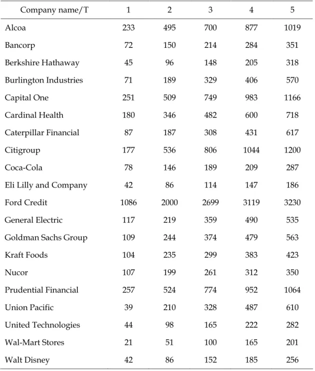
Company name/T 1 2 3 4 5 Alcoa 233 495 700 877 1019 Bancorp 72 150 214 284 351 Berkshire Hathaway 45 96 148 205 318 Burlington Industries 71 189 329 406 570 Capital One 251 509 749 983 1166 Cardinal Health 180 346 482 600 718 Caterpillar Financial 87 187 308 431 617 Citigroup 177 536 806 1044 1200 Coca-Cola 78 146 189 209 287
Eli Lilly and Company 42 86 114 147 186
Ford Credit 1086 2000 2699 3119 3230
General Electric 117 219 359 490 535
Goldman Sachs Group 109 244 374 479 563
Kraft Foods 104 235 299 383 423 Nucor 107 199 261 312 350 Prudential Financial 257 524 774 952 1064 Union Pacific 39 210 328 487 610 United Technologies 44 98 165 222 282 Wal-Mart Stores 21 51 100 165 201 Walt Disney 42 86 152 185 256
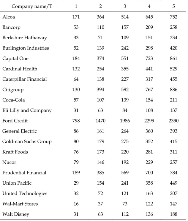
Company name/T 1 2 3 4 5 Alcoa 171 364 514 645 752 Bancorp 53 110 157 209 258 Berkshire Hathaway 33 71 109 151 234 Burlington Industries 52 139 242 298 420 Capital One 184 374 551 723 861 Cardinal Health 132 254 355 441 529 Caterpillar Financial 64 138 227 317 455 Citigroup 130 394 592 767 886 Coca-Cola 57 107 139 154 211
Eli Lilly and Company 31 63 84 108 137
Ford Credit 798 1470 1986 2299 2390
General Electric 86 161 264 360 393
Goldman Sachs Group 80 179 275 352 415
Kraft Foods 76 173 220 281 311 Nucor 79 146 192 229 257 Prudential Financial 189 385 569 700 784 Union Pacific 29 154 241 358 449 United Technologies 32 72 121 163 207 Wal-Mart Stores 16 37 73 122 147 Walt Disney 31 63 112 136 188
Company name/T 1 2 3 4 5 Alcoa 119 253 357 448 524 Bancorp 37 76 109 145 180 Berkshire Hathaway 23 49 76 105 163 Burlington Industries 36 96 168 207 293 Capital One 128 260 383 502 601 Cardinal Health 92 176 246 307 369 Caterpillar Financial 44 96 157 220 317 Citigroup 90 274 411 533 618 Coca-Cola 40 75 96 107 147
Eli Lilly and Company 22 44 58 75 95
Ford Credit 554 1021 1381 1602 1672
General Electric 60 112 183 250 274
Goldman Sachs Group 55 125 191 245 289
Kraft Foods 53 120 153 195 217 Nucor 55 102 133 159 179 Prudential Financial 131 267 395 487 547 Union Pacific 20 107 168 249 313 United Technologies 23 50 84 113 144 Wal-Mart Stores 11 26 51 84 102 Walt Disney 21 44 78 95 131
4.3.4. Theoretical CDS spread and Quoted CDS spread
Alcoa Ford Credit
T Quoted R=0.3 R=0.4 R=0.5 T Quoted R=0.3 R=0.4 R=0.5 1 475 233 171 119 1 1349 1086 798 554 2 503 495 364 253 2 1176 2000 1470 1021 3 522 700 514 357 3 1068 2699 1986 1381 4 531 877 645 448 4 988 3119 2299 1602 5 558 1019 752 524 5 966 3230 2390 1672
Bancorp General Electric
T Quoted R=0.3 R=0.4 R=0.5 T Quoted R=0.3 R=0.4 R=0.5 1 NA 72 53 37 1 NA 117 86 60 2 NA 150 110 76 2 NA 219 161 112 3 NA 214 157 109 3 NA 359 264 183 4 NA 284 209 145 4 NA 490 360 250 5 NA 351 258 180 5 NA 535 393 274
Berkshire Hathaway Goldman Sachs Group
T Quoted R=0.3 R=0.4 R=0.5 T Quoted R=0.3 R=0.4 R=0.5 1 352 45 33 23 1 186 109 80 55 2 345 96 71 49 2 181 244 179 125 3 338 148 109 76 3 180 374 275 191 4 327 205 151 105 4 183 479 352 245 5 321 318 234 163 5 184 563 415 289
Burlington Industries Kraft Foods
T Quoted R=0.3 R=0.4 R=0.5 T Quoted R=0.3 R=0.4 R=0.5
1 NA 71 52 36 1 50 104 76 53
2 NA 189 139 96 2 58 235 173 120
3 NA 329 242 168 3 61 299 220 153
5 NA 570 420 293 5 73 423 311 217
Capital One Nucor
T Quoted R=0.3 R=0.4 R=0.5 T Quoted R=0.3 R=0.4 R=0.5 1 302 251 184 128 1 72 107 79 55 2 261 509 374 260 2 80 199 146 102 3 247 749 551 383 3 89 261 192 133 4 227 983 723 502 4 97 312 229 159 5 215 1166 861 601 5 102 350 257 179
Cardinal Health Prudential Financial
T Quoted R=0.3 R=0.4 R=0.5 T Quoted R=0.3 R=0.4 R=0.5 1 43 180 132 92 1 519 257 189 131 2 46 346 254 176 2 541 524 385 267 3 48 482 355 246 3 565 774 569 395 4 51 600 441 307 4 581 952 700 487 5 52 718 529 369 5 590 1064 784 547
Caterpillar Financial Union Pacific
T Quoted R=0.3 R=0.4 R=0.5 T Quoted R=0.3 R=0.4 R=0.5 1 246 87 64 44 1 61 39 29 20 2 248 187 138 96 2 66 210 154 107 3 249 308 227 157 3 68 328 241 168 4 250 431 317 220 4 71 487 358 249 5 251 617 455 317 5 73 610 449 313
Citigroup United Technologies
T Quoted R=0.3 R=0.4 R=0.5 T Quoted R=0.3 R=0.4 R=0.5 1 486 177 130 90 1 50 44 32 23 2 452 536 394 274 2 55 98 72 50 3 440 806 592 411 3 59 165 121 84 4 424 1044 767 533 4 65 222 163 113 5 413 1200 886 618 5 73 282 207 144
Coca-Cola Wal-Mart Stores T Quoted R=0.3 R=0.4 R=0.5 T Quoted R=0.3 R=0.4 R=0.5 1 33 78 57 40 1 59 21 16 11 2 43 146 107 75 2 69 51 37 26 3 48 189 139 96 3 72 100 73 51 4 55 209 154 107 4 77 165 122 84 5 60 287 211 147 5 79 201 147 102
Eli Lilly and Company Walt Disney
T Quoted R=0.3 R=0.4 R=0.5 T Quoted R=0.3 R=0.4 R=0.5 1 37 42 31 22 1 60 42 31 21 2 40 86 63 44 2 60 86 63 44 3 44 114 84 58 3 61 152 112 78 4 46 147 108 75 4 64 185 136 95 5 48 186 137 95 5 66 256 188 131
The result from the evaluation is presented in table 2, 3, 4, 5, 6, 7 and 8. We can see when we inspect the results from the calculations of the risk-neutral default probabilities that the recovery rate assumption has an impact on the result. The probabilities of default are negatively correlated to the assumption about the recovery rate. We can see that the difference is greater with longer times to maturity. Ford for example experiences a difference in result of 46.36% compares to 33.12% when the recovery rate is 30% and 50% respectively with five year to maturity. The same results, with one year to maturity are default probabilities of 15.51% and 11.08% i.e. recovery rate assumption have an increasing effect with time to maturity. Examining the result we can see that Ford had the notably highest probability of default and Wal-Mart exhibiting the lowest default probability. If we look at the results from the calculated CDS spreads we can see that all of the companies of course have increasing spread over time, this is due to the feature of the model. What also can be observed is that all companies experience a convex
increase in spread over time. All companies have of course a negative correlation between spread and recovery rate. Looking at the tables where quoted CDS data is presented alongside the calculated results we can observe that the calculated results broadly tend to underestimate the CDS spread for shorter times to maturities and overestimate for longer time to maturities. This goes for almost all bonds and follows from the fact that quoted CDS spreads barely increases over time, something that the quoted ones do. The reason behind this will be discussed later on in the analysis.
5. Analysis
5.1. Interpretation of the Results
Given the results that we have presented in the tables a clear pattern can be discovered. The obvious finding when spreads are calculated with the Hull and White model (2000) is that they are always increasing over time. There are no results acquired where we exhibit a decreasing spread over time or even a flat curve. This is obvious when we look upon how the model is constructed, since the model assumes that the corporate bond spread only captures default risk. This implies that cumulative probability has to increase at all times and that is what it will do as long as the corporate bond spreads are higher than the Treasury bonds. If this is not the case the model will give negative probabilities of default at times when the corporate bond yields a lower return than the Treasury rate. Given the quoted CDS data of almost all companies we have to conclude that this is a rather limited feature of the model. Since almost all quoted CDS data exhibit a very limited increase over time and in some cases it even decreases. This gives us reason to believe that the real CDS price incorporates other factors in the pricing mechanism and that the default probability measure does not consider having a strict positive relationship with time. When we look closer at for example the quoted data
on Citigroup and Capital One we note that they actually have a decreasing spread over time. This implies that investors assume a higher risk of default in the near future and an increasing default probability over time. The reason behind this phenomenon might be closely linked to business cycles and the assumption that the aftermath from the recent economic meltdown gives investors reason to assume that default is decreasing over time. This is something that the model is incapable to absorb due to its construction. Our findings conclude that the Hull and White model (2000), given the assumptions used have an approach towards how investors look at risk, with increasing risk aversion over time. This has to be matched to the current situation at the time when the bond prices were collected. This was at the late peak of the credit crisis when investor’s attitude towards risk has to be viewed as somewhat alternative to what’s normally assumed. With this in mind we could explain some of the discrepancies between the calculated results and the quoted CDS spreads.
Another factor that might play part in how risk-neutral default probabilities are calculated is the fact that we are unable to construct a bootstrapped zero-curve from the corporate bonds. This is due to shortage of zero-coupon bonds needed for the procedure. It is debatable though if this would have made any difference in the observed calculated results.
5.2. Analysis of pricing error
Pricing errors mainly come from four factors: unrealistic assumptions of the model, inappropriate proxies as model inputs, poor data quality, and the inaccurate techniques used when the model is applied.
According to the fundamental assumption of Hull and White model, the credit spread captures only credit risk of the reference entity, which means, in a risk neutral world, at time t, the premium on a credit default swap for a
given reference entity with a term expiring at T should be equal to the yield on a par bond issued by the reference entity with maturity at time T minus the yield on a par non-defaultable bond with maturity at time T, or
CDS Premium(t,T) = Corporate Par Yield(t,T) – non-defaultable Par Yield(t,T)
This implies that, in a frictionless market, if the CDS premium exceeds the par yield spread, an arbitrage profit could be captured by forming a portfolio that is long a default-free bond, short a corporate bond and short a CDS. If the CDS premium is less than the par yield spread, the opposite positions capture the arbitrage profits.
However, a consensus has been reached that yield spread include, apart from credit risk, a liquidity premium, if nothing else, therefore the yield spread include a default component and a non-default component. From the results acquired it seems quite obvious that the non-defaultable component in the yield spread plays a rather big role and is hence affecting the results in a negative way. It can be argued that the non-default part seems to increase over time as the life of the bond gets bigger.
The second factor of pricing errors goes hand in hand with the first factor. Government bonds, in most cases, the U.S. Treasury is considered the proxy of non-defaultable bond in credit models. However, using Treasury yield as model input increases the non-default component of the yield spread. First of all, U.S. Treasury bonds are among the most liquid securities in the world, while some corporate bonds trade only rarely, if at all. (here we can have a chart comparing trading volume of treasury and some of our bonds) If the corporate bond market prices liquidity, then the differential liquidity between the corporate bond market and Treasury market can cause a non-default premium to arise in the corporate bond market. Also, the return on corporate bonds is in most cases riskier than the return on government bonds therefore investors demand a risk premium for investing in corporate
bonds and that this risk premium is responsible for the non-default portion of the yield spread. The systematic portion of non-default component of corporate bond yield has been empirically tested using Fama and French factors and explains the non-default component of corporate bond yield positive. Thirdly, interest payments on government bonds are not taxed at the state level, while interest payments from corporate bonds are subject to state taxation. This asymmetric tax treatment causes higher-coupon rate corporate bonds ask for a larger spread as compensation. However, we don’t make any distinctions on bonds with different coupon rates. Furthermore, we interpolate the yields of bonds issued by the same reference entity regardless of coupon rate to get the zero curve, which may cause the cross-sectional comparison on spread/premium less meaningful.
The bond data we use as model inputs is of rather poor quality. Subjecting to non-frequent trading, market segmentation, inefficient bond market, we believe that some bonds are not correctly priced. Furthermore, all our bond data is sourced from Thomson Datastream, which quotes pricing from a single dealer instead of actual trade prices from the market as a whole therefore there is a potential for bias.
Some of the techniques we use to implement the model are not very appropriate as well. As described before, we calculate the Treasury zero curve. However, in order to attain the zero-curves for corporate bonds, linear interpolation is needed at times, particularly when there are only a small amount of bonds issued by a reference entity, since the Treasury and corporate bonds to be compared with yield curves should have the exact same time to maturity. To get a corresponding corporate curve to the zero curve we obtained, we need to find bonds that mature at the same dates as the Treasury bonds which we use to bootstrap the Treasury zero curve, in order to get the yield spread hence calculate the risk-neutral default probabilities. To come around this problem, two corporate bonds are chosen.
One that matures as close prior to the Treasury and another one that matures as close subsequently as possible. From these two bonds a linear interpolation is made to find a new bond price that matches the given date of the Treasury. With the interpolated result there is a possibility to compare the yield of the Treasury with to corporate on and out of that get a measurement of the probability that’s sought after.
6. Conclusion
With the simplifying assumptions of the Hull and White model, we managed to calculate a number of static CDS spread for all 20 companies in our sample. However, comparing to the quoted CDS spread on the market, the model seems not performing well. Since the model is based on a theoretical structure it is incapable of adjusting to situations where factors deviate from the given assumptions, like investors attitude towards risk. This limits the accuracy of the results to only apply when conditions are suitable.
References
Altman, E., Kishore, V. (1996). Almost everything you wanted to know about recoveries on defaulted bonds, Financial Analysts Journal, 52-(6): 57-64.
Black, F., Cox, J. (1976). Valuing Corporate Securities: Some Effects of Bond Indenture Provisions, Journal of Finance, 31-(2), 351-367.
Cetin, U., Jarrow, R., Protter, P., Yildirim, Y. (2004). Modeling Credit Risk with Partial Information, Annals of Applied Probability, 14-(3), 1167-1178.
Duffie, D. (1999). Credit swap valuation, Financial Analysts Journal, 55-(1),
73-87.
Duffie, D., Singleton, K. (1999). Modeling Term Structures of Defaultable Bonds, Review of Financial Studies, 12-(4), 687-720.
Geske, R. (1977). The Valuation of Corporate Liabilities as Compound Options, Journal of Financial and Quantitative Analysis, 12-(4), 541-552.
Gifford, F., Vasicek, O. (1984). A Risk Minimizing Strategy for Portfolio Immunization, Journal of Finance, 39-(5), 1541-1547.
Hull, J., White, A. (1995). The impact of default risk on the prices of options and other derivative securities, Journal of Banking & Finance, 19-(2), 299-323. Hull, J., White, A. (2000). Valuing credit default swaps 1: No counterparty default risk, Journal of Derivatives, 8-(1), 29-40.
Iben, T., Litterman, R. (1991). Corporate Bond Valuation and the Term Structure of Credit Spreads, Journal of Portfolio Management, 17-(3), 52.
Jarrow, R., Turnbull, S. (1995). Pricing Derivatives on Financial Securities Subject to Credit Risk,Journal of Finance, 50-(1), 53-85.
Jarrow, R., Lando, D., Turnbull, S. (1997). A Markov Model for the Term Structure of Credit Risk Spreads, Review of Financial Studies, 10-(2), 481-523. Kim, I., Ramaswamy, K., Sundaresan, S. (1993). Does default risk in coupons affect the valuation of corporate bonds?: A contingent claims model, Financial Management, 22-(3), 117-132.
Derivatives Research, 2-(2), 99-120.
Longstaff, F., Schwartz, E. (1995). Valuing credit derivatives, Journal of Fixed Income, 5-(1),6-13.
Merton, R. (1974). On the Pricing of Corporate Debt: The Risk Structure of Interest Rates,Journal of Finance, 29-(2), 449-470.
O’Kane, D., Turnbull, S. (2003). Valuation of Credit Default Swaps, Quantitative Credit Research, 2003-Q1/Q2
Appendix 1. Companies included in the study
Company Name Industry Credit Rating
Alcoa Aluminum BBB-/Baa3
Bancorp Financial services BB+/Baa1
Berkshire Hathaway Financial services AAA
Burlington Industries Textile manufacturer A/Aa2
Capital One Financial services BBB/Baa1
Cardinal Health Drug Wholesale BBB+/Baa3
Caterpillar Financial Financial services A/A2
Citigroup Financial services C
Coca-Cola Beverage A/Aa2
Eli Lilly and Company Pharmaceuticals & Healthcare AA/A1
Ford Credit Financial services CCC+
General Electric Conglomerate AA+/Aa2
Goldman Sachs Group Financial services A
Kraft Foods Food Processing BBB+/Baa2
Nucor Steel & Iron A/A1
Prudential Financial Financial services Baa2
Union Pacific Transportation BBB/Baa2
United Technologies Conglomerates A/A2
Wal-Mart Stores Retailing AA/Aa2
Appendix 2. Empirical findings on recovery rate Industry Average Recovery Rate % Public Utilities 70.5
Chemical, petroleum, rubber and plastic products 62.7 Machinery, instrments and related products 48.7 Services - business and personal 46.2
Food and kindred products 45.3
Wholesale and retail trade 44.0
Diversified namufacturing 42.3
Casino, hotel and recreation 40.2
Building material, metals and fabricated products 38.8 Transportation and transportation equipment 38.4 Communication, broadcasting, movie production 37.1
Financial institutions 35.7
Construction and real estate 35.3
General merchandise stores 33.2
Mining and petroleum drilling 33.0
Textile and apparel products 31.7
Wood, paper and leather products 29.8
Lodging, hospitals and nursing facilities 26.5
Total 41.0
Altman & Kishore, Stern School NYU)
This is the base paper on defaulted corporate bonds over the period 1971-1995. It came up with a wide range of differing recovery rates, by industry, as shown below.
Appendix 3. Graphs on theoretical and quoted CDS spread Alcoa 0 200 400 600 800 1000 1200 1 2 3 4 5 quoted CDS spread R=0.3 R=0.4 R=0.5 Ford Credit 0 500 1000 1500 2000 2500 3000 3500 1 2 3 4 5 Quoted CDS R=0.3 R=0.4 R=0.5
Berkshire Hathaway 0 50 100 150 200 250 300 350 400 1 2 3 4 5 Quoted CDS R=0.3 R=0.4 R=0.5
Goldman Sachs Group
0 100 200 300 400 500 600 1 2 3 4 5 Quoted CDS R=0.3 R=0.4 R=0.5 Kraft Foods 0 100 200 300 400 500 1 2 3 4 5 Quoted CDS R=0.3 R=0.4 R=0.5
Capital One 0 200 400 600 800 1000 1200 1400 1 2 3 4 5 Quoted CDS R=0.3 R=0.4 R=0.5 Nucor 0 50 100 150 200 250 300 350 400 1 2 3 4 5 Quoted CDS R=0.3 R=0.4 R=0.5
Cardinal Health 0 100 200 300 400 500 600 700 800 1 2 3 4 5 Quoted CDS R=0.3 R=0.4 R=0.5 Prudentiao Financial 0 200 400 600 800 1000 1200 1 2 3 4 5 Quoted CDS R=0.3 R=0.4 R=0.5
Caterpillar Financial 0 100 200 300 400 500 600 700 1 2 3 4 5 Quoted CDS R=0.3 R=0.4 R=0.5 Union Pacific 0 100 200 300 400 500 600 700 1 2 3 4 5 Quoted CDS R=0.3 R=0.4 R=0.5