Portfolio Policies with Stock Options
Yuliya Plyakha‡ Grigory Vilkov§
This version: May 8, 2008 First Version: January 2008
Abstract
We study the partial equilibrium portfolio optimization problem for a myopic CRRA investor who can trade options on individual stocks. Applying the parametric port-folio approach of Brandt, Santa-Clara, and Valkanov (forthcoming) to derivatives, we show that options characteristics (such as implied volatility and IV smile skew) convey information about the mispricing in the option portfolios. We take the data on all US-traded options to build characteristic-based factor portfolios of options. An investor uses them in addition to the market portfolio and Fama and French (1992) factors in her utility maximization. Surprisingly, portfolios based on the IV smile skew turn out to be less important than IV-based portfolios, and factor port-folios from call options are in general more interesting for an investor than the factors from puts. Market frictions in the form of stock shortsale constraints are compensated by the use of options, and having options with no stock shortsales allowed may be better than having only stocks with shortsales permitted. Monthly rebalancing leads to extreme transaction costs for an investor facing the full bid-ask spread, providing limits to arbitrage interpretation of the documented mispricing in the option portfolios.
Keywords: stock options, portfolio analysis, hedge fund policy, implied volatility, skew risk
JEL: C21, G13, G14
‡Graduate Program ’Finance and Monetary Economics’, Goethe University, Mertonstr. 17, Uni- Pf
77, D-60054 Frankfurt am Main, Germany. E-mail: [email protected]
§Goethe University, Finance Department, Mertonstr. 17-21, D-60054 Frankfurt am Main, Germany
and INSEAD, Finance Department, Boulevard de Constance, F-77305 Fontainebleau, France. E-mail: [email protected]
We would like to thank Christian Schlag for support and timely advice. We are also grateful to Joost Driessen, Massimo Massa, Joel Peress, Astrid Schornick and seminar participants at INSEAD and Uni-versity of Frankfurt for their multiple comments and help. Grigory Vilkov would especially like to thank his PhD advisor Pascal Maenhout for guidance, support and helpful comments. All remaining errors are our own.
1
Introduction
Individual stock options represent an important class of financial assets. In one-factor models like Black and Scholes (1973) and Merton (1973), the plain option is just a lever-aged position in underlying with an implicit insurance against adverse stock movements. In reality, options violate assumptions of one-factor models and fit multi-factor mod-els with stochastic volatility (Heston (1993), Bates (2000), among others) and/or jumps (Bates (1988), Bakshi, Cao, and Chen (1997) and others).
In this case we have several possible scenarios: an option-specific factor is systemati-cally priced, i.e., an option with higher exposure to such a factor bears a systematisystemati-cally different risk premium in its return; an option-specific factor is not priced and the associ-ated risk is not interesting for an investor; or an option-specific factor is not systematically priced, but an investor would receive exposure to it due to an irrational but long-lasting mispricing.1 It is important to be able to isolate such factors empirically, i.e., to find the proxies (instrumental variables) that allow us to approximate the factors from the options’ payoff space.
In this paper we attempt to solve this problem by maximizing the CRRA utility for a myopic investor having access to the US exchange-traded individual options and underlying stocks.2 Our main contribution is that we use a very extensive dataset of stock
options (on about 5,000 underlyings) to bridge and extend two strands of literature on empirical option pricing: research that deals with preference-free analysis of the option pricing anomalies, and preference-based portfolio analysis with derivatives. We identify the characteristic-based factors from the options return space that benefit an investor with the CRRA utility. We are also able to interpret the optimal factor combinations intuitively in the form of commonly used trading strategies.
Our second contribution is an application of the parametric portfolio policy approach (Brandt, Santa-Clara, and Valkanov (forthcoming)) in the setup with individual options. We show that it is a powerful tool to build factors from the existing payoff space and to use them in the investor’s optimization problem. It allows us to reduce the dimensionality of the optimization problem from a large number of assets to a significantly smaller number of factors, or characteristics, that we use to build those factors.
The bulk of recent empirical option pricing studies concentrate on index options. Bon-darenko (2003), Constantinides, Jackwerth, and Perrakis (forthcoming), and Bakshi and Kapadia (2003b), among others, document violations of one-factor model assumptions and confirm the negative sign of the variance risk premium for index options. The limited research on individual stock options has not come to an agreement regarding the sign and nature of variance risk premia yet, and we hope to set guidelines by providing new evidence on stock option-based factors. Bakshi and Kapadia (2003a) study 25 individual equity options and find that their prices embed a negative market volatility risk premium, but the magnitude of this risk premium is small. Driessen, Maenhout, and Vilkov (2007)
1A considerable mispricing may exist for a long time due to transaction costs, and this limits of
arbitrage argument is consistent with the empirical results in Section 6.3.
2The form of preferences is not a crucial assumption in our partial equilibrium setup. We mainly use
a specific utility function in order to compare the portfolio return distributions to reach an optimum. We could have compared the moments of distributions directly, but it would be more difficult to achieve the optimal ordering of portfolio policies.
look at options on all S&P100 component stocks and do not find economically signif-icant returns for those in excess of the one-factor model. Carr and Wu (forthcoming) investigate the synthesized variance risk swaps for 35 individual securities. They find a large cross-sectional variation in variance risk premia, and conclude that the majority of the market variance risk premium is generated by an independent variance risk factor. Goyal and Saretto (2007) study short-term ATM options on individual stocks and find an economically important source of mispricing in the options’ implied volatilities. They conclude that zero-cost trading strategies in options constructed on the base of variance risk premium proxy produce a significant average monthly return.
We extend this literature in two dimensions. First, we confirm that on an economy-wide scale with all exchange-traded stock options, the options on individual stocks are not simple leveraged substitutes (with insurance) for stock risk factors, and that option returns are partly driven by independent risk factors. Second, we show that risk factors for options of different moneyness/maturity/type profiles may not be strongly correlated, and this opens a Pandora’s Box with respect to modeling options’ dynamics. What we fail to show for now is that these factors are indeed systematic; this important question is left for further research.
Previous research shows that options may indeed represent a lucrative asset class for different investors. Liu and Pan (2003) find that access to derivatives influences optimal stock holdings, improves the portfolio performance, and plays an important role in utility maximization for non-myopic investors. Driessen and Maenhout (2007) empirically study the problem of portfolio choice with OTM puts and ATM straddles investments. They consider several types of investors and find that all of them should optimally have short positions in the derivatives in order to earn the jump and volatility risks premia. Haugh and Lo (2001) use the idea of the Black-Scholes option pricing model to construct buy-and-hold portfolios consisting of bonds, stocks and options. They are not able to analyze a large number of options, but find that options are interesting for an investor under various underlying models and types of preferences. Most of the research on portfolio choice works with stocks, bonds and index options. Our analysis is different in two dimensions. First, we use a much larger dataset of individual options, and second, we do not allow investors to take outright (i.e., just long or short) positions in options. We build factor portfolios from the options assigned to several asset classes (with a similar maturity/moneyness/option type profile), and each of those portfolios represents an approximately market delta neutral long-short spread trade.
The direct maximization of utility for an investor who also invests in derivatives is a very complex problem. A great amount of research is focused now on finding the ways to simplify the portfolio optimization problem. Instead of focusing on the properties of distribution of returns of the assets in the portfolio, we take the direction similar to Brandt (1999), Ait-Sahalia and Brandt (2001) and Brandt, Santa-Clara, and Valkanov (forthcoming). Brandt (1999) solves the problem of finding portfolio weights such that expectation of marginal utility is equal to zero, conditional upon forecasting variables and without making any assumptions on how returns depend on those variables. Ait-Sahalia and Brandt (2001) argue that the best approach would be to choose variables that are able to predict portfolio weights directly rather than the first to try to predict returns. Using a semiparametric approach to construct an index from the default spread, the log of the dividend-to-price ratio, the term spread, and the momentum, they look for
an optimal portfolio in terms of this index composition.
Building on the previous results, we perform our analysis in the following steps. First, we select the characteristics of the options and underlying securities that may convey information about the priced risk factors. For stocks they are traditionally size, book-to-market (Fama and French (1992)), and momentum (Carhart (1997)). For options we use the level of implied volatility and the skew size as characteristics.3
Second, we divide all options into the standard asset classes by moneyness (OTM and ATM), time to maturity (short- and long-dated) and option type (calls and puts). For each asset class we create quantile-based factor portfolios for each of the two characteristics.4
Interestingly, many pairs of the resulting factor returns have a very low correlation, and cannot be treated as substitutes. Potentially, this can lead us to a hypothesis that puts and calls, for example, are in part driven by different risk factors. We also estimate the risk premia on these factors in stocks and options portfolios. It turns out that many of the identified factors indeed contribute systematically to option returns, while not having a significant effect upon stock returns.
Third, we use the parametric portfolio approach of Brandt, Santa-Clara, and Valkanov (forthcoming) and work with portfolio weights in a form of a function of the assets’ characteristics. Effectively, we make our portfolio weights a function of 1) the assets’ weights in factor portfolios (as a parameter), and 2) the decision variableθ that represents the weight of each factor portfolio. Solving the investor’s optimization problem for θ, we can find the weights of the underlying assets (if we need to). Surprisingly, it turns out that for a CRRA investor, most interesting factors are derived from implied volatility as a sorting variable, and many interesting factor combinations are built using call options (while most options’ mispricing results in the literature are related to put options).
The paper proceeds as follows. In the next section we briefly discuss the general ideas of the parametric portfolio policies approach of Brandt, Santa-Clara, and Valkanov (forth-coming) and then apply these ideas to a portfolio optimization problem with derivatives. In section 3 we describe our data and discuss how we prepare it for further analysis, applying various filters and aggregation. In section 4 we talk about the intuition behind choosing particular asset characteristics to build factors, show how we create the factor portfolios and elaborate on our expectations from portfolio optimization with these fac-tors. In section 5 we explore the solution to the investor’s problem. We show the optimal trading strategies and try to estimate risk premia on option-based factors. In section 6 we introduce several extensions and also discuss the impact of market friction on the investor’s actions. Finally, section 7 concludes.
3As the implied volatility (IV) measure we take the constant volatility from the fitted binomial tree
Cox, Ross, and Rubinstein (1979) with discrete dividends for American options and the usual Black and Scholes (1973) IV for European options. As the skew measure we use the difference between the IV of the OTM and ATM options
4We use characteristics as conditioning variables, i.e., we condition the factor portfolio composition in
2
Parametric Portfolio Policy
In this section we discuss the general idea of the parametric portfolio choice methodology, and show the formal setup of the optimization problem. The approach allows for the easy application of the investor’s problem within a large universe of assets whose dynamic is driven by a number of common factors.
2.1
General Idea
Following Brandt, Santa-Clara, and Valkanov (forthcoming), we model portfolio weights directly as a function of a set of asset characteristics. A representative investor holds the market and then optimizes her final portfolio composition with respect to the specified factors derived from the asset returns and respective characteristics. We should note that in this paper we limit ourselves to linear factors, though it has been shown (Jones (2006)) that option returns follow a non-linear factor structure.
The average utility, from consuming the portfolio return in each period, over a given time frame is an objective function of an investor, and is maximized over the weights of factor portfolios in the total portfolio, or, in other words, over the loadings (denoted by θ
- constant over time) on the assets’ characteristics.
This scheme effectively decreases the dimension of the optimization problem from a large number of assets in the investor’s universe to a relatively small number of factors. An important feature of this approach is that it is very general and allows for easy extensions. The inclusion of new factors merely represents a problem of computational capacity.
Brandt, Santa-Clara, and Valkanov (forthcoming) suggest the application of the para-metric portfolio policy approach to bond or currency portfolios, using the characteristics of these assets as choice variables. Instead, we add derivatives to the assets universe of a CRRA investor, i.e., we will explore the implications of giving the investor access to the options-based factors. Interesting issues include the choice of factors maximizing the average utility, and interaction between the choice of stock- and option-based factors.
Next, we look at the formal setup of the investor’s optimization problem in the para-metric portfolio approach.
2.2
The Model
Consider an investor who wants to form her portfolio using individual stocks and options. Every monthithere areJs
i stocks in the economy andJidderivatives, so the total number of assets equalsJi =Jis+Jid. The investor maximizes her conditional utility from consuming the portfolio return for each time period (month) i:
max {ωi,j}Jij=1 Ei[u(ri+1,p)] = Ei " u Ji X j=1 ωi,jri+1,j !# . (1)
Hereωi,j is the weight of asset j at time i, ri,p is the portfolio return at time i, and ri,j is the periodic return of asset j at time i.
We follow and extend the parametric approach of Brandt, Santa-Clara, and Valkanov (forthcoming) and construct portfolio weights ωi,j for stocks and derivatives as a function of their characteristics ωi,j =f(¯ωi,j, xsi,j, xdi,j, θ), where
f(¯ωi,j, xsi,j, x d i,j, θ) = ¯ ωi,j, 1 Js i θTxsi,j, 1 Jd i θTxdi,j , (2)
where ¯ωi,j is the weight of asset j at time i in the value-weighted market portfolio, xsi,j is the vector of characteristics of stock j at time i, xdi,j is the vector of characteristics of derivative j at time i, and θ is the vector that gives loads on the characteristics and has to be estimated.
As we use the same vectorθfor stocks and derivatives in equation (2), then formally the following should be true:dim(θ) =dim(xs
i,j) anddim(θ) = dim(xdi,j). We construct vectors
xs
i,j and xdi,j to have the same dimensions as θ and with zeroes on the last dim(θ)−Ks elements ofxsi,j for the stocks’ characteristics, whereKsis the number of factors considered for stocks. This is similar for derivatives’ characteristics: the first dim(θ)−Kd elements of vector xd
i,j are zeroes,Kd is the number of factors considered for derivatives:
xsi,j = (xs,i,j1, ..., xs,Ki,j s, 0, ...,0 | {z } dim(θ)−Ks )T, xdi,j = ( 0, ...,0 | {z } dim(θ)−Kd , xd,i,j1, ..., xd,Ki,j d)T
and the following holds: dim(θ) = Ks+Kd.
Note that θ is chosen to be constant through the time, which means that portfolio weights are time dependent only to the extent of the time dependency of ¯ωi,j and the characteristics of stocks and derivatives.
If we define the market portfolio as the benchmark, then the terms J1s iθ Txs i,j and 1 Jd i θTxd
i,j can be considered as deviations from the benchmark portfolio. We standardize stocks’ and derivatives’ characteristics so that their cross-sectional distribution becomes stationary. As a result the cross-sectional means J1s
i PJs i j=1θTxsi,j and J1d i PJd i j=1θTxdi,j are zero, compatible with an interpretation of the factor portfolio investment as deviation from the benchmark portfolio. The following equation holds by construction:
Ji X j=1 f(¯ωi,j, xsi,j, x d i,j, θ)·13×1 = Ji X j=1 ¯ ωi,j+ 1 Js i θTxsi,j+ 1 Jd i θTxdi,j = 1,
where 13×1 is a vector-column of ones. We denote ri+1,j = (rsi+1,j, ris+1,j, rdi+1,j)T, where
rs
i+1,j and rid+1,j are returns at time i+ 1 on stock j and derivativej respectively.
Since θ does not depend on time, instead of maximizing the investor’s conditional utility in equation (1), it is enough to maximize her unconditional (or mean myopic) utility over θ: 1 T T−1 X i=0 u(ri+1,p) ! = 1 T T−1 X i=0 u Ji X j=1 f(¯ωi,j, xsi,j, x d i,j, θ)·ri+1,j !
= 1 T T−1 X i=0 u Ji X j=1 ¯ ωi,j+ 1 Js i θTxsi,j+ 1 Jd i θTxdi,j ri+1,j ! . (3)
We do not impose constraints on ¯ωi,j yet, so that short selling is allowed. We study the implications of the shortsale constraints below in Section 6.1.
This approach can be applied in many different ways depending on how one treats char-acteristics. The most straightforward is to invest in the characteristics directly. Consider, for example, the first element of vectorθ(it corresponds to the first stock’s characteristic)
θ1. Then the amount J1s iθ1x
s
i,j will be invested into the first characteristic (it could be the size characteristic of the stock) of stock j at time i. Our empirical studies will be based on investing into factor portfolios (see details in Section (4).
We consider an investor with CRRA utility function
u(ri+1,j) = 1 + ¯ωi,jrsi+1,j+ 1 Js i θTxs i,jrsi+1,j+ 1 Jd i θTxd i,jrid+1,j 1−γ 1−γ .
To solve the maximization problem (3) we apply the Generalized Method of Moments (GMM). The moment conditions for the stocks’ characteristics only are the following:
1 T T−1 X i=0 ∂u(ri+1,p) ∂θk = 1 T T−1 X i=0 " u0(ri+1,p)· 1 Js i Ji X j=1 xs,ki,jri+1,j # = 0,
whereθk fork ∈Ksis the weight of thek-th characteristic of stocks in the portfolio, where the k-th characteristic of stock j ∈ Jis at time i is equal to xs,ki,j. The moment conditions for the derivatives part can be defined in a similar manner. The Hessian matrix of second derivatives in the case when l ∈Ks and m∈Kd is equal to
1 T T−1 X i=0 ∂u2(r i+1,p) ∂θl∂θm = 1 T T−1 X i=0 " u00(ri+1,p)· 1 Js i Ji X j=1 xs,li,jri+1,j ! · 1 Jd i Ji X j=1 xd,mi,j ri+1,j !# .
We analyze the significance of the estimatedθ-parameters and utility gains from adding the new factors into the base case portfolio optimization in order to test if inclusion of the new factor improves the investment strategy.
Our benchmark portfolio is the market. We can rewrite the returns on the optimal portfolio in the following way:
ri+1,p = Ji X j=1 ¯ ωi,jri+1,j+ Ji X j=1 1 Js i θTxsi,j ri+1,j+ Ji X j=1 1 Jd i θTxdi,j ri+1,j =ri+1,m+rsi+1,h+r d i+1,h,
i.e., it is the sum of the return on the market portfolio and of the return on a zero-cost portfolio that consists of two parts: equity (rs
i+1,h) and derivatives (rdi+1,h). It is possible to interpret the problem (1) as the utility maximization of an investor who already holds the market and wants to invest in a market-neutral derivatives hedge fund.
3
Data Description
For the portfolio selection problem of an investor we take individual stocks and plain vanilla options written on them as the assets. We restrict the universe of US stocks to those that have traded options within the 1996−2004 time frame. To construct factor port-folios we use a number of company- and asset-related characteristics. The data processing procedures, i.e., initial selection, various filters we apply and variables we construct, are described in detail for stocks and options separately.
3.1
Stock Data
We use Compustat as the main source for quarterly company-related data, and CRSP for information on monthly and daily stock returns and shares outstanding each month. Selecting only the US stocks with traded options, we end up with 4964 stocks and initially download the data for them from January 1995 to December 2004. We use the following notation: i∈ {1, ...,108} - time index and j ∈ {1, ...,4964} - firm index.
We follow Brandt, Santa-Clara, and Valkanov (forthcoming) in forming the monthly stock factors from Compustat/CRSP variables. The exact definition of these variables can be found in Appendix A. From Compustat we get the values for assets, liabilities, common and preferred stocks, and deferred taxes. If the price of a common stock does not exist in Compustat, we take it from CRSP. In the Compustat table returns are given monthly, and the rest of the variables are quarterly. To get monthly data we apply linear interpolation of quarterly values, and we do so for assets, liabilities, preferred stock value, and deferred taxes. As a result, for these variables we get time series of 108-month (from January 1996 to December 2004) for 4964 stocks and use them to form the appropriate stock characteristics each month.
We define book equity as equal to total assets minus liabilities plus balance sheet deferred taxes and investment tax credits minus preferred stock value. Market equity is equal to price per share times shares outstanding. We omit observations with negative market or book equity values. Book-to-market (BTM) is then equal to the log of book equity divided by market equity. Size characteristic (ME) is computed as the log of market equity. We also calculate momentum each month for all available stocks on a rolling basis using the monthly returns over the past year asM OMi =Qi
−2
k=i−13(1 +rp,k). For the 1996
year momentum we use monthly returns for 1995-1996 from CRSP.
3.2
Options Data
We use OptionMetrics to get monthly data for put and call options from January 1996 until December 2004. Since we have already restricted the universe of stocks to those having options, it is not surprising that we have options on the same number of underlyings as the number of stocks, i.e., on 4964.
We work with raw data, i.e., with best bid and ask closing quotes rather than the interpolated volatility surfaces constructed by OptionMetrics. We select all options having 10 to 180 days to maturity, and then we discard options with zero open interest or with
zero bid prices. To eliminate evident pricing errors we also remove the options with implied volatilities higher than 100%.
We are interested in monthly holding period returns, and we construct these taking into account the American feature of traded stock options. To calculate the returnro
i,j for a given option o on underlying j in month i we use the price of that option at the end of the previous month and compare it with the value of the option at the end of a given month. The value of an option is the maximum of its price and the value of the immediate exercise.
Using different prices we also make an attempt to study the effect of the transaction costs on the portfolio policy. For the returns with zero transaction costs we use mid quotes as prices (i.e.,(best bid+best offer)/2). For returns with transaction costs we take as the initial price the best bid for a short position in options and the best offer for a long position. Then we close these positions on the other side of the bid-ask spread at the end of the month, i.e., for the short position we take the max(best offer, value of immediate
exercise), which is effectively equivalent to best offer, and for the long position we take
the max(best bid, value of immediate exercise).
Usually a stock in our dataset has several options outstanding on a given day, with var-ious strikes, expiration dates, and types (put or call). Dealing with each option separately is quite difficult as they are often not cross-sectionally comparable along moneyness and maturity dimensions. To standardize the choice of options for an investor we construct three moneyness5 and two maturity buckets (corresponding to [0.85, 0.95], (0.95, 1.05] and (1.05, 1.15] moneyness levels and [10, 90], (90, 180] days to maturity) for calls and puts appropriately. Then we sort all options into corresponding buckets and aggregate options on one underlying into one security. We treat each bucket as the investable asset class with its calculated implied volatility and return. For the return and volatility cal-culations on aggregated options we assume equally weighted investments in all options on the same underlying assigned to a given bucket at a given time. On average there are about 200 aggregated options in each bucket at each point in time.
4
Factors and Predictions
The idea of parameterizing portfolio weights is a simplification of a general portfolio optimization problem. Of course, an important issue is the choice of factors with respect to which we perform the optimization. Our approach is based on the features of stocks and derivatives markets and existing literature that tries to simplify the investor’s optimization problem and to go around the task of modeling the distribution of portfolio returns.
4.1
Choice of Characteristics
For the stocks the choice of characteristics is relatively straightforward, based on previ-ous research. We consider size (market capitalization), book-to-market ratio (Fama and French (1992)) and momentum (Carhart (1997), Daniel and Titman (1997), Jegadeesh
5Where moneyness is defined for each options as a relation of strike (K) to spot price (S), i.e., K
and Titman (2001) among others). We regard this choice as a base case and add a num-ber of derivatives with their respective characteristics (read, factors) to the investor’s investment opportunity set.
Brandt, Santa-Clara, and Valkanov (forthcoming) investigate how the behavior of an investor would change if she considers interactions between stock-based factors. Instead we concentrate on the factors that stem from derivatives’ characteristics. We expect them to improve the performance of an investor’s portfolio.
In an extension we also look at the effect of the stock shortsale constraints (sections 6.1) and at the stock’s liquidity factor (section 6.2). We also test the validity of the results for a portfolio with derivatives where an investor is paying the full bid-ask spread at each rebalancing date (section 6.3). We do not consider a transaction costs factor explicitly, although it might have interesting interaction effects with other characteristics and serve as a proxy for the derivatives’ liquidity factor. We leave this issue for later research.
To choose the options’ characteristics we simply regard options as the derivatives written on the underlying stocks. Under the assumption of an Ito process for the stock S, driven by a multidimensional Brownian motion dWS
t and possibly a jump process dJt
dSt
St
= (µ−λE[ξt])dt+σtdWtS+ξidJi,
the derivative security return will be driven by the same Brownian motion and the same jump process. In addition, if the diffusion coefficient σt by itself is stochastic, i.e., its dynamics can be described by an SDE, as for example in the Heston (1993) model,
dσ2t =κ(θ−σt2)dt+ςσtdWtσ, dW S t dW
σ
t =ρtdt,
the SDE for derivative asset inherits the factors driving the diffusion coefficient (and correlation ρt between the Brownians if it is stochastic as well) by the simple application of Ito’s lemma. The same holds true for jumps: the option’s SDE inherits the jump process from the stock, and furthermore if the jump size/intensity are stochastic, their driving processes will show up in the SDE for derivative securityQ as well.
Qs−Q0 = Z s 0 ∂Qt ∂t dt+ ∂Qs ∂St dSt+ 1 2 ∂2Qt ∂S2 t [dSt] 2 + ∂Qt ∂σ2 t dσt2+1 2 ∂2Qt ∂(σ2 t) 2 dσ2t2+ ∂ 2Q t ∂St∂σ2t dStdσt2 + X 0<τ≤t {Q(S(τ))−Q(S(τ−))}.
Thus, the option returns in this setup will be driven by underlying in a leveraged fashion as well as by stochastic volatility and/or jump processes. If an investor first buys the market portfolio, and then only adjusts her appetite for direct stock-based factors like ME, BTM, and MOM, she does not normally need options. However, after taking the risks represented by the stock’s Brownian motion WtS, she may want to go for pure volatility/jump risk factors, and hence build up positions in options. We recognize this and build our factors for derivatives using a proxy for volatility and jump risks priced in
options.6 Reasonable proxies for this purpose are the implied volatility from the
Black-Scholes model (Black and Black-Scholes (1973)) for European options or from the binomial tree (Cox, Ross, and Rubinstein (1979)) for American options, and the skew size measure. Im-plied volatility level and volatility smile across moneyness and time convey information on factors affecting option returns directly and through the leveraged underlying’s continuous risk factors. This intuition is confirmed by several studies of the option markets.
Carr and Wu (forthcoming) show that the part of the market risk factor is correlated with the return variance, and that ME, BTM, and MOM risk factors can explain only a small portion of the documented variance risk premia. The authors conclude that the market variance should be largely driven by risk factors independent of those driving the underlying returns. Thus, we expect other factors, probably built on the existing assets like options, to be able to explain the returns of derivative assets.
The CAPM fails to explain why small and value stocks tend to be underpriced. Pietro and Vainberg (2006) study how firm characteristics like size and book-to-market relate to equity option expensiveness and check if these characteristics influence the pricing of systematic variance risk in the equity options market. They find that under the same level of expected realized variance under physical measure, options on small stocks are more expensive than options on large stocks, and that options on value stocks are more expensive than options on growth stocks. The authors claim that overestimation of risk on small and value stocks leads investors to demand higher rates of returns on these types of stock, and propose to also study the influence of momentum earnings on options pricing. Implied volatility tends to be higher for small firms, as well as for high book-to-market ratio firms. Duan and Wei (forthcoming) show that a higher amount of systematic risk leads to a higher level of implied volatility and a steeper slope of the implied volatility curve. Following these findings, we can expect some interaction between IV and skew size factor on the one side, and BTM, ME, and MOM factors for stocks on the other side.
Our choice of the second characteristic of the derivative assets is additionally supported by the work of Bates (2001), who views the options markets as an insurance market for crash risk. Deriving myopic portfolio allocation, he concludes that equity and crash insurance are complements in the event of large negative jumps on the market. Branger, Breuer, and Schlag (2006) look at the optimal exposures to volatility and jump factors in a semi-simulated environment, and confirm that an investor with CRRA utility optimally chooses to take exposure to jump and volatility risks under discrete rebalancing conditions. Thus, we find it reasonable to choose the level of implied volatility and a measure of the smile skew, calculated as the difference between the implied volatility for OTM and ATM options, as characteristics for the derivative assets. We call it a skew or a crash factor, although it only corresponds to a crash factor for put options, and for call options it’s rather a factor of positive jump or of an effect of stochastic volatility.
6As we discuss below in Section 4.3, our option-based factors are approximately delta-neutral by
construction, and hence we indeed deal with the variance risk or small changes in underlying and can hope for some variance risk factor identification that is not priced in stocks.
4.2
Building Factor Portfolios
We define an asset class as the collection of financial instruments with a predetermined payoff, maturity, and moneyness profile. For example, we can define a class of all out-of-the-money call options with maturity between 10 and 90 days, and so on. As de-scribed above, we construct three moneyness and two maturity buckets (corresponding to [0.85, 0.95], (0.95, 1.05] and (1.05, 1.15] moneyness level intervals and [10, 90], (90, 180] days to maturity intervals) for calls and puts appropriately. Each of the buckets represents an investable asset class.
After we have defined the characteristics for a given asset class, we start building factors. For each factor portfolio we would like to get equally weighted exposure to the assets in extreme quantiles, with a positive sign in the extreme upper quantile, and with a negative sign in the lower one. For every date i we form three quantiles for the char-acteristics and assign the values −1, 0 and +1 to lower, middle and upper thirds. These values correspond to thexasset
i,j ’s in the portfolio weight definition (2). Then we divide each element of the vector xs
i,j (for stocks) andxdi,j (for derivatives) by the number of elements in the corresponding quantile. By construction, normalized dummies x
s i,j Js i and xd i,j Jd i cross-sectionally sum up to 0 when the number of elements in the upper and lower quantiles is equal, which can easily be achieved. We then treat these normalized quantiles as asset weights for the factor portfolios corresponding to a given characteristic of a specified asset class. The decision variableθ manages our exposure to each factor portfolio, and the goal is to optimize the investor’s utility with respect to θ.
Thus, we define factor portfolios with respect to the characteristics of an asset class. It follows that in the given setup we limit the option strategies of investors to long/short positions in options of the same type (calls or puts), long/short synthetic forwards (whenθ
for the same moneyness and maturity calls and puts is of a different sign, but has the same absolute value), and long/short strangles (when θ for the same moneyness and maturity calls and puts are of the same sign and same absolute value). Maturity differences also imply some horizontal spreads in forwards and strangles. In Tables 1 and 2 we provide examples of attainable strategies for differentθcombinations. We do not include straddles or single options in our set of investable strategies, as has been done in the literature (e.g., in Driessen and Maenhout (2007)). Our main goal is to construct factor portfolios from options that improve the investor’s asset allocation, and to test if the resulting factors bear a systematic risk premium in traded assets. Our main goal is to find systematic factors in options that allow the investor to improve her asset allocation.
4.3
Predictions and Expectations
As discussed earlier, we start with the market portfolio and then maximize the investor’s utility by using the enlarged investment opportunity set with a number of additional factors. For the stocks we take ME, BTM, and MOM factors, and for options we create factors for each asset class based on implied volatility level and skew size.
Though we have a relatively short sample period, for the stock factors we do not expect to obtain results which differ from previous research. The investor would deviate from the market by investing in small stocks and finance this purchase shorting large cap
stocks (Fama and French (1992), Fama and French (1996)), by buying value stocks and stocks outperforming the market in the past, and finance it by selling growth and stocks that did not perform well in the last 12 month (Jegadeesh and Titman (1993), Jegadeesh and Titman (2001), Carhart (1997)).
For options we have two characteristics - the level of implied volatility and the volatility smile skew measure - applied to 12 asset classes (3×2×2 = moneyness×maturity buckets for calls and puts). When we create factor portfolios for options, we build approximately delta-neutral positions as within each asset class we buy and sell options of about the same delta level. It makes our factor portfolio immune to small changes in the price of the underlying, and thus roughly isolates the volatility risk factor.
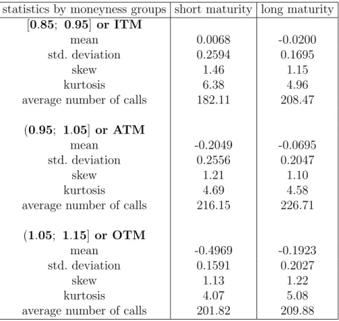
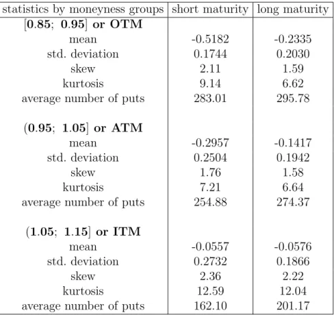
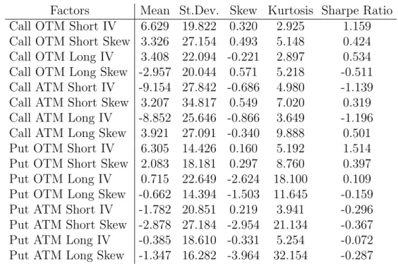
From the literature we know that OTM and ATM options tend to be mispriced (or we face the peso problem as in Branger and Schlag (2005)) as respective asset classes with respect to standard asset pricing models (Constantinides, Jackwerth, and Perrakis (forthcoming), Bondarenko (2003), and an investor optimally sells those options (Driessen and Maenhout (2007) among others). Tables 3 and 4 provide statistics on all the investable asset classes we created. For individual options the mean return is quite negative and the distribution has pronounced fat tails. Returns are positively skewed and very volatile. OTM options show more negative returns than ATM and ITM contracts. Table 5 shows the statistics for the option factor portfolios we created. Overall their distribution has very fat tails and is mostly negatively skewed; some of the factors should be interesting for investors (judging by the Sharpe Ratios with absolute magnitude above 1).
For our purpose it does not matter if the option group is mispriced with respect to some asset-pricing model, since we do not allow the investor to go short or long for all options in an asset class. Instead, we are looking at the mispricing of options within one asset class with respect to the average for this class, and try to infer priced factors (for an investor with a given utility function) from this mispricing. For asset classes with fairly priced volatility and jump risks we still expect to see no systematic preference of one options group over the other, i.e., we would expect the θ-estimates to be insignificant.
From all asset classes we select only those containing OTM and ATM options. ITM options effectively resemble the leveraged position in the underlying, and we want to study the options with larger time value relative to the option price, i.e., higher compensation for the risks of the option seller. Thus, we are left with four moneyness and maturity buckets, two for calls and puts respectively.
As we talk about volatility and skew risks (whatever their real sources are), it makes sense to sell options with higher volatility and skew characteristic values. It makes more sense to sell options with a high risk premium on these factors, but under the assumption that the risk premium is proportional to the levels, we can treat levels of skew and volatilities as premium proxies.
In Section 5 we will see if this intuition is confirmed by the empirical findings.
5
Results
In this section we discuss the results and see if our previous intuition is confirmed by the empirical findings. First we look at the base case with only stock factors available,
then we move to extensions with various option-based factors. It is important to keep in mind that interpretation of the values, especially the sign of θ parameters, depends upon the ranking of the correspondingly sorted cross-sectional characteristics for a given asset class. For example, for the stocks, negative θ means going short stocks with a high value of a given characteristic and long stock with a low value of the characteristic. For options positive θ means being long options with a high value and short options with a low value of the characteristic. If we take the level of implied volatility as the characteristic for an asset class containing short maturity ATM put options and we find positive optimalθ, we will buy puts with a relatively high volatility and sell puts of this bucket with a relatively low volatility.
5.1
Base Case
We consider investment into equities as the base case, which means we buy the market and then take care of three main stock factors: size (ME), book-to-market (BTM), and momentum (MOM). The results are in line with previous research and our intuition. Brandt, Santa-Clara, and Valkanov (forthcoming)(BSCV) obtain as optimal estimate for
θ the vector:
(θme, θbtm, θmom) = (−1.220, 3.466, 2.00),
for the CRRA case withγ = 5. For the same risk aversion we getθ = (−1.559, 2.469, 2.130). Taking into account different data used for estimations, we can say that our results are in line with previous research. An investor would deviate from the market by being long small stocks, value stocks, and past winners (and short large caps, growth and past losers respectively).
Adding the option-based asset classes and factors to the investor’s investment oppor-tunity set in the next subsection, we investigate the appetite of an investor to volatility and skew risk factors.
5.2
Stocks and Options
We do not investigate options separately from stocks, since we hope to capture factors common to stocks and options through the ME, BTM, and MOM factors.
Table 6 shows the time series correlations between the factor portfolios based on various asset classes. We should be careful in choosing the factor portfolio combinations for the optimization problem, since factors based on the same characteristic for different asset classes may be highly correlated. If we see that investors are taking opposite positions in these factors, we may face a collinearity bias. The good news is that the option-based factors are hardly correlated with the stock-based factors, so they do not seem to be substitutes for each other. The maximum absolute correlation is 0.38, while the maximum correlation between the stock-based factors is much higher, with a value of 0.72 between MOM and BTM. The factors based on calls and puts are close to independent between option types, with a maximum absolute correlation of 0.39 for all pairs, and we can freely mix them in the portfolio. We can also combine certain IV factors with skew factors for calls and puts, but it seems dangerous to include several IV factors for the same option type.
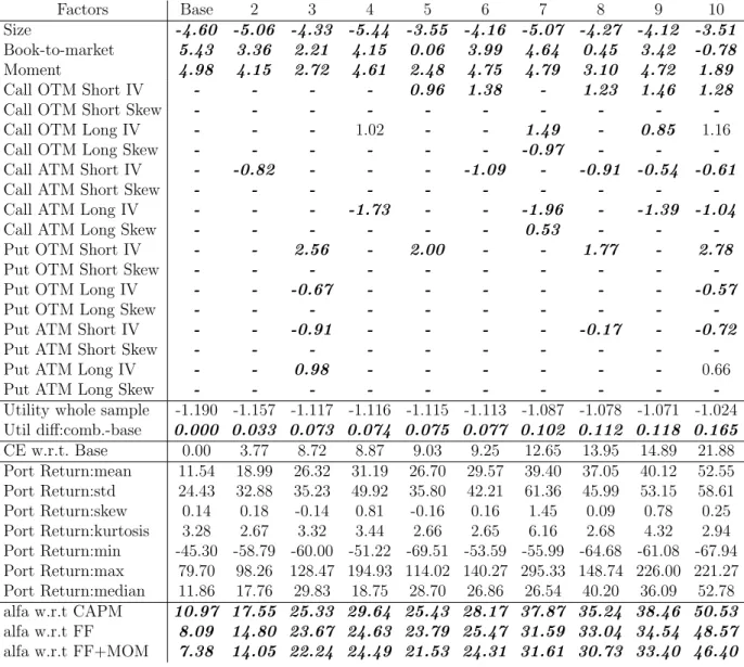
To identify interesting factor combinations we look at several measures shown in Tables 7-8 for different levels of risk aversion. First, after solving the maximization problem of an investor for the whole sample period from January 1996 to December 2004 (107 months), we achieve portfolio composition with optimal levels of θ. For each optimal portfolio we calculate distributional characteristics of returns over the whole sample period, mean utility level, and look at the utility gain from adding option-based factors to the base case. We discard the combinations that do not result in significant utility gain over the whole sample period.7 To test the stability of estimations we also solve the optimization problem over the first 2/3 of the sample period (i.e., 72 months) and compare the utility calculated with θs of the 72 month period to the utility over the remaining 35 months using the θ
estimates of the first 72 months. We discard the factor combinations, resulting in different mean utility levels over the last 35 months depending on the θ estimation period.
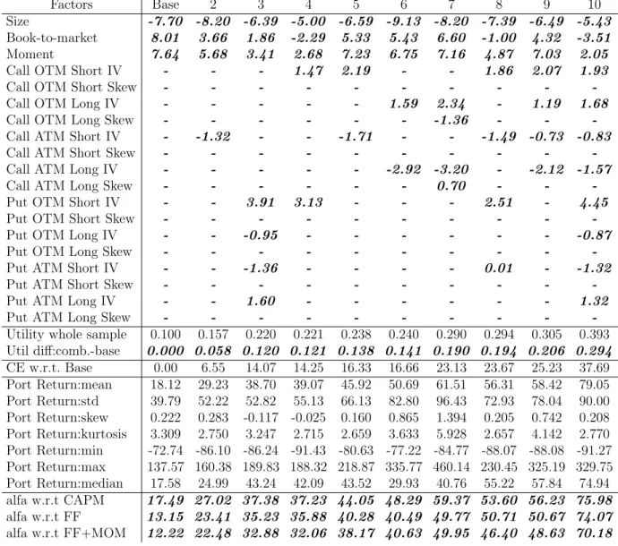
From the surviving combinations8 we select 10 for the exposition. This last choice is not fully ad hoc: we first take the combinations with as few option-based factors as possible, and it gives us 4 portfolios with 2 or fewer option-based factors and the rest with 4 or more. The Tables 7-8 already contain filtered combinations, i.e., only those that pass the utility gain and stability tests. All these combinations are potentially interesting for further analysis as all of them result in significant positive α with respect to linear factor models (with FF and momentum factors).9
Surfing the tables, we can point out the following regularities. First, higher risk aversion leads to lower θ’s, i.e., smaller deviations from the market portfolio. Overall this gives more modest returns and smaller risks expressed by standard deviation of the portfolio returns over time. Second, there are not many extreme positions with opposite signs in option factor portfolios, so collinearity does not seem to be a problem for the surviving combinations.
Looking broadly at theθ values, we can summarize the following findings. Contrary to common belief, we do not find many significantθs based on the skew (crash) characteristic of the options. If there is some dispersion in volatility/jump pricing for the selected asset classes, we can barely identify it using the skew size. We will be selling skew factor for long-term OTM calls, buying some of it for long-term ATM calls. This means that volatility/jump risk premia are too high for long-term OTM calls with a large skew and/or too low for the same options with a small skew. For long-term ATM calls the risk premium is too high for low skew options. Interestingly, for put options the crash factor looks even worse: we get the best significance for short ATM puts, while the common belief is that short OTM puts pricing is heavily driven by crash fears. In any case, crash factors never seem to be working alone, and normally show up in combination with the IV-based factors. Implied volatility seems to be more important as the characteristic variable for most asset classes, and the inclusion of just one asset class IV factor can lead to a significant
7We test the significance of the utility gain by comparing the means of utility time series for a given
factor combination and the base case for the whole sample period.
8Depending on risk aversion we have a different number of valid factor combinations passing all tests.
Forγ∈ {1, 1.8}we have 25 and 23 combinations respectively. Full results can be provided upon request.
9Base case scenario also shows a positiveα, though it is based on the same four factors that we use
for regression. It is due to difference in factors: in our investor optimization problem we use factors built from our stock sample, while in factor regressions we use ready-to-use factors from Kenneth R. French’s web-site.
utility improvement over the base case (as we see in the combination 2 in Tables 7 and 8). With the IV characteristic for options at our disposal, we will be buying either short- or long-dated OTM calls’ factor portfolios, and/or selling either short- or long-dated ATM calls’ factor portfolios. A long position in short-dated OTM put factors also benefit an investor, while the long-dated puts-based portfolios do not contribute much.
It is hard to name the most important factor as there is obviously a lot of interplay between them. The combinations with more factors included make the investor generally better off in terms of utility (if we do not take into account associated transaction costs from monthly rebalancing). Comparing calls and puts, we come to the conclusion that there is more mispricing in the call-based portfolios than in the put-based ones. Using only one ATM calls portfolio derived from IV as a characteristic, the investor significantly improves her utility, reaping an additional 3.77% certainty equivalent (expressed as a percentage of the initial wealth) over the base case for the γ = 1.8 (Table 8). Just two call-based portfolios, as in combinations 4, 5, 6, work better for an investor than four put-based portfolios, as in the combination 3.
Including all possible factors in the investor’s optimization problem makes her even better off, but most θs end up being not significant (except for the log utility case). Based on the informal analysis of how many times the theta for a given factor shows up significantly in the estimations,10 we assign the trading signals to a given characteristic
quantile. The results are given in Table 9, and confirm our previous findings that call-based factors are more important for an investor. Within the calls the long-dated options give more interesting factor portfolios than short-dated ones. We have three strong signals and one without grade for long-dated calls vs. two strong and two weak for short-dated ones.
To offer the reader some additional information on the option-based factors, in Tables 1 and 2 we also provide an interpretation of pairwise factor combinations in the form of spread trading strategies. Most of them look plausible and are easy to construct, e.g., a characteristic spread in strangles, where we buy (sell) strangles for all options with a low value of a characteristic, and sell (buy) strangles for all options with a high value of the same characteristic. The combination 5 in Table 8 is exactly this kind of strategy: we are buying short maturity strangles with high volatility and finance them by selling the strangles of the same maturity with low volatility. The combinations 4 and 6 in the same table represent a characteristic spread in vertical spreads, where we buy vertical spreads on calls with low volatility and sell them with high volatility (for long and short maturities respectively). The combination 2 is just a factor portfolio, and the others are hard to interpret. Thus, we use our initial factor portfolios as building blocks for more complex strategies and note that these strategies can also be used as building blocks to reach a new level of complexity.
Following Pietro and Vainberg (2006) we can also expect interaction effects between the option and stock factors. In the current setup we can identify the option asset classes where the option-based factors are substitutes for the stock factors in the investor’s prob-lem. Size factorθ does not seem to fluctuate much across the combinations, and it always remains significantly negative for all risk aversion levels. The other two stock factor θs
10Here we take into consideration all 23 surviving factor combinations forγ= 1.8 and not only those
are less stable. The first θ responsible for BTM factor drops by most from the base case level with the addition of short OTM puts IV factor, and does even lose significance for a number of combinations. The other θ corresponding to momentum also drops with the inclusion of the same OTM put IV factor, but not that significantly. It provides us with in-direct evidence that there is a relationship between the pricing of volatility in short-dates OTM puts and the value vs. growth anomaly in stock returns. The correlation between the corresponding factors is quite low (0.23 for BTM and short OTM puts IV factor), so the relationship must be non-linear. One way of looking into the issue deeper would be the direct estimation of the factor risk premium in stock returns, and this is left for further research. It can also be interesting to test if some simple non-linear functional dependency of carefully chosen factors gives us a reasonable explanation of documented interaction.
The above discussion is based on the results in an ideal environment for an investor, where she does not face any transaction costs in the form of bid-ask spread, nor has she any shortsale constraints on stocks. The liquidity of the market for a given instrument may also influence investment strategy. In the following sections we also try to shed light on the optimal portfolio with market frictions.
5.3
Factor Premia Estimation
As we have seen from the interaction between stock- and option-based factor portfolios in the previous section, as noted in previous research (Ang, Hodrick, Xing, and Zhang (2006), Xing, Zhang, and Zhao (2007) among others), parameters of the underlying’s process (realized volatility or observed jumps as proxy for it) and its observed effect on options characteristics (skew in the risk neutral probability distribution, or IV smile skew size as its proxy) can reveal important asset pricing factors, either systematic or resulting from a sustained mispricing. Pricing errors (α) in the portfolio return with respect to common linear factor (market, 3 FF, and 3 FF + momentum) models confirm this intuition. As we see in Tables 7 and 8, each portfolio combination demonstrates a highly significant positive α over each of the generally accepted linear models.
We are going to estimate the risk premia on the factors derived from option asset classes with appropriate characteristics and see if these factors are systematically priced in stocks and in options. There are several possibilities for the outcome: first, option-based factors may be priced in both stocks and options; second, they may be priced in options, but not priced in stocks; and third, they can be priced in either stocks or options, or in both, but the estimations may not be robust. The first two outcomes are interesting and both have important implications. The last outcome may be due to a short estimation period, or may hint at the sustained mispricing in the option factor portfolios. It would make option portfolios interesting for an investor, but they will not be loading on any systematic factors.
The first decision we have to make is what factors and what asset returns we take. We have seen in Table 6 that many factors for different asset classes are highly correlated, and there is little sense in estimating risk premium for all of them at the same time. The model will be definitely misspecified as options have non-linear factor structure (Jones (2006)), and it is not our purpose here to describe it completely. All we want to do is see if linear
factors based on option characteristics bear a significant risk premium affecting option returns directly or through stock returns. We have seen in Tables 7-8 and 9 that the most interesting factor portfolios are based on IV level for OTM calls (both short and long dated), IV level for ATM calls (again both maturities), the skew size for long-dated OTM calls, and the IV level of short-dated OTM puts. Our working hypothesis would be that these factors represent priced systematic risk factors for option returns. We would expect the IV from the OTM short puts factor to be priced in stocks through its interaction with the BTM factor.
For better diagnosis of what factors are important, we estimate risk premia for each option-based factor individually. We follow standard two-stage Fama and MacBeth (1973) procedure and include three FF factors (Fama and French (1992)), momentum (Carhart (1997)), and one of the option-based factors. To be consistent with other asset-pricing literature we use not the self-made factors, but rather download the ready-to-use ones from Kenneth R. French’s web-site. We use returns on all options in the defined asset classes,11 and all 4964 time series of stock returns used in the paper to form standard portfolios. We first build 3 portfolios for each of the option asset classes using the full-sample estimated option factor β as a sorting variable. It gives us 36 derivatives portfolios. Then we build 30 portfolios from stocks, following the same procedure and using the estimated factorβ
as a sorting variable. In the second stage we infer the factor risk premia with GLS (using the variance-covariance matrix of first stage residuals as weighting matrix as suggested by Shanken (1985) among others) from 36 option portfolios and 30 stock portfolios separately. In Table 10 we show the estimated risk premia on the market, three Fama-French and momentum factors, plus one selected option-based factor. In Table 11 we also show the summary results for estimated risk premium on option-based factors using 36 option and 30 stock portfolios, as well as the t-statistics calculated with Shanken (1992) correction in both cases.
We should be very careful in drawing any strict conclusions from the results. As we noted, the tests are definitely ill specified (as we can see from large significantα’s in each regression), the portfolio returns and factors are too volatile, and the time series are rather short (only 107 months) to identify the factor risk premia with confidence. After we correct the second step regression standard errors for errors in estimated betas (due to Shanken (1992)), we hardly derive any significance, even for standard factors. The risk premia in stocks are not big enough in the first place to be able to split into so many components using limited series length. In options, the risk premia are larger in magnitude (due to their leveraged nature), and we derive sufficient significance after all necessary standard error corrections. However, when we compare the calculated risk premia for option-based candidate factors with the time series mean of the respective factors in Table 5, we see that the estimations are not nearly at the level that they should be. Thus, we should either increase the sample length or come up with another testing method.
Our exercise still delivers some interesting results concerning the standard linear fac-tors we used in the estimation. The risk premia estimations for SMB and MOM facfac-tors are mixed, while the estimations for the market and for HML risk premia are very stable, and the HML risk premium is everywhere negative. The mean value of the HML stock factor is positive, and hence the value premium estimates from stocks and options are not
11As we have described in section 3.2, we have 3 moneyness×2 maturity×2 option type buckets and
consistent. Several explanations may support the findings. First, Arshanapalli, Fabozzi, and Nelson (2006) show that the value premium can turn statistically negative in stocks in the strong market. The US market from 1996 until 2004 experienced hard times, but still grew about 100% in these years (if we look at the S&P100 index). Option buyers may be overestimating the prospects of the economy in comparison to the stock buyers, and hence they may be implicitly pricing the negative value premium in the options. Second, there may be higher replication costs for options on the firms in distress (or in general high value firms), and this leads to lower returns on options. The second point can be verified empirically, and we intend to do so in later research.
6
Extensions
This section discusses how our previous analysis changes if we introduce some real-life con-ditions into our optimization problem.12We talk about shortsale constraints and
liquidity-related issues for stocks, and then also make an investor pay the full bid-ask spread while rebalancing derivatives-based factor portfolios.
6.1
Constrained Optimization
We assume in our analysis that we have a sophisticated investor, and she has access to all markets and can carry out all possible trades. However, even sophisticated investors will not be able to short the stocks if there are no stocks to borrow. This may happen in the small cap markets or under certain adverse market conditions. If there are options on a stock, one can always take a synthetic forward position to gain access to the underlying risk. We investigate how the portfolio composition is going to change from the previous optimization if we impose the shortsale constraints on stocks. As we restrict the investor’s assets choice to factor portfolios instead of direct option positions, creating forwards for some stocks may not be possible.
We solve the optimization problem using the same GMM routine as before, with an additional condition that the optimal weight of any given stock j at each time i in the portfolio should be non-negative:13
¯ ωi,j+ 1 Js i θTxsi,j ≥0, ∀i∈ {1, ...,107}, ∀j{1, ...,4964}.
This additional constraint transforms into the formal number of 4,964∗107 = 531,148 inequalities (in reality there are fewer inequalities due to missing returns), and the solution
12While we will be mostly talking about the constrained investor problem, please note that the investor
has been constrained in her choice from the very beginning due to an incomplete market. The market is incomplete as we use options as non-redundant assets in addition to the stock market and try to optimize investor utility with respect to unknown factors. When we introduce additional frictions, we just reduce the attainable payoff space even more.
13The optimization setup is misspecified to some degree here as an investor may not know the value
of the characteristic in the remote future. However, asθs are assumed to be constant over time, we have
to impose this forward-looking restriction. Another way to model it would be to optimize with non-negativity constraints, assuming today’s values of characteristics, and later just trim the stock holdings at zero if they are optimally negative.
is very time consuming. As a consequence, we only solve the problem for several interesting factor combinations.
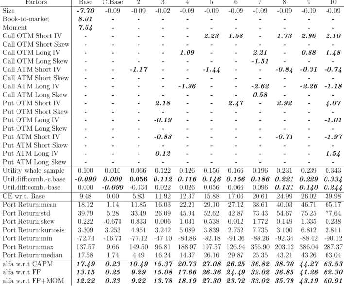
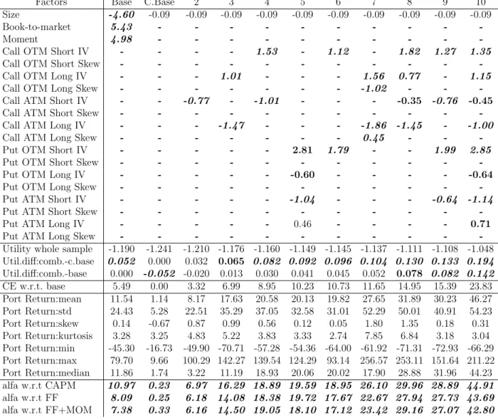
The summary results are provided in Tables 12-13. We select for exposition the same combinations as in the unconstrained case, though again we gain more significant results. Two points are worth mentioning. First, the stock weights’ non-negativity constraints are binding, and the investor now mostly refuses to invest in stock factors, except for ME. θ estimations for BTM and MOM are not significantly different from 0, while for ME,θ is very similar across all estimated combinations (and significant for the log utility case). The ME factor is dominating the others, and an investor tries to go short the ME factor portfolio. However, the non-negative weight constraints should stop her very fast. Second, option-based factors compensate for stocks constraints, and in all but one case (combination 2 forγ = 1.8, Table 13) we get significant utility improvement over the base constraint case. Moreover, in three cases for each risk aversion level we derive a significant utility improvement over the unrestricted base case. Such strategies involve four and more option factor portfolios, and hance may be overstating the utility gains due to transaction costs.
The results for the significance of the optionθs estimations resemble, to a large extent, the unconstrained case: an investor chooses IV-based portfolios, where all estimatedθs are significant, while the crash factor does not seem to be adding much to the investor’s utility. Crash factor θs are significant in combinations with IV factors only, e.g., combination 7 in Tables 12-13.
Interestingly, the magnitude of estimated absolute θs is smaller for the constrained case. Two explanations arise: first, this is the way to compensate for the reduced stock factor holdings, i.e., there is an interaction between the stock and options factor portfolios. Second, options are riskier investment vehicles by themselves, and now we invest less in them as we reduced relatively safer stock investment.
In general we can say that to a large extent, option-based factors allow an investor to overcome the short-sale constraints. Again, IV-based factors prove to be more important than crash factors.
6.2
Stock Liquidity Factor
In this section we form the liquidity factor for stocks following Pastor and Stambaugh (2003). They construct a liquidity measure that reflects temporary price changes accom-panying order flow and find that the aggregate liquidity is a priced state variable in the economy.
We use this approach to study if liquidity is a priced factor in the portfolio with option-based factors and if options can compensate using their leveraged nature for the liquidity of the underlying stocks. We do not claim that this is the only way to account for liquidity in the portfolio optimization; instead we insist that the methodology is flexible and allows the inclusion of many other factors. We estimate liquidity using the following OLS regression:
d = 1, ..., D, where ri,d,j is the return on stock j on day d in month i, and ri,d,je is the excess return over the market represented by the CRSP value-weighted index,vi,d,j is the dollar trading volume (in millions) for stock j on day d in month i. Then the estimated coefficient ξi,j is the stock’s j liquidity in month i, and it is calculated only if there are more than 15 return observations in a given month.
Intuitively, large stocks are more liquid than small ones. The first inspection of our results confirms this intuition through the correlation of 0.51 between liquidity and size factors (Table 6). Liquidity is also positively correlated with both the value factor (0.18) and momentum (0.19). The latter is in line with the suggestions of Pastor and Stambaugh (2003).
It is interesting that the estimate of liquidity-θ only appears to be significant in the base case if the risk-aversion coefficient is equal to 1 (log-utility). Including all the factors in our portfolio optimization under the same level of risk aversion does not gain much of the utility from adding liquidity as a factor (0.5387 with liquidity and 0.5384 without it). For the risk aversion of 5, the significance of the liquidity factor in the portfolio is not high enough, but can be considered in the portfolio if ATM short maturity IV calls factors are included in the portfolio, sometimes together with the OTM short maturity IV puts factor. Both θ parameters of these factor portfolios are negative.
The general tendency of the θ estimates for the factor combinations with liquidity is the same as described in the section (5.2). However, we have to point out thatθ estimates for liquidity are very high for some combinations of factors,
6.3
Transaction Costs
Evidently, transaction costs affect the investment policy, and we investigate if investors can adapt knowing that they face a bid-ask spread on each rebalancing date. Even for large stocks in the S&P100 index the average bid-ask spread fluctuates between 3% for deep ITM puts, 7% for ATM puts, and 42% for deep OTM puts (Horn, Schneider, and Vilkov (2007)), and for small stocks in our sample the rebalancing costs may even be worse.
We approach the problem from two different angles. First, we check what happens to the portfolio performance if the investor optimizes using the mid-price returns and then in reality faces the bid-ask spread. Second, we let the investor know in advance that each month she will only get the ask-to-bid return on the long options’ positions, and the bid-to-ask return on the short options’ positions.
The first approach leads to complete deterioration of the portfolio performance, and this is not surprising with such frequent rebalancing and noted bid-ask spreads. Mean returns on the portfolio vary from −6.9% for strategies with only a few ATM option’-based factors to −745% in cases when OTM options are added. A cure may be to go for a less frequent rebalancing policy, or to opt for no rebalancing at all.
We try another trick: we provide an investor with data on returns assuming real bid-ask spreads on long and on short positions. Again we assume that an investor liquidates all old positions at the end of a month and creates new ones after that, each time incurring the full bid-ask spread. This assumption is not very realistic as part of the last month’s
positions will most probably survive into the next month and no real transaction will take place. We want to see if the options markets remain lucrative under these conditions.
It turns out that an investor is able to adapt partially: her portfolio returns are mostly positive and range from about −2% to 11.54%. However, an investor is still not able to attain a higher utility than by just investing in stock-based factors. The bottom line is that facing real transaction costs, an investor has to optimize not only to risk factors, but also to a rebalancing frequency. However, advanced market participants able to trade at mid-market or better can benefit from the analysis in this paper.
7
Conclusion
Individual stock options represent an important class of financial assets, and investors are looking for ways to identify the trading rules for them. We show empirically that stock option characteristics (such as the implied volatility and the volatility smile skew) contain information on the mispricing in the option portfolios. We build option factor portfolios based on these characteristics, and an individual investor with CRRA utility function can use them to improve her utility. In contrast with the previous research we use a very extensive option prices dataset and directly solve an investor utility maximization problem.
As a second contribution, we apply a methodology of Brandt, Santa-Clara, and Valka-nov (forthcoming) to the portfolio selection with stock options. This allows us to reduce the dimensionality of an investor’s optimization problem from the number of assets to a limited number of factor/asset class combinations. We form eight investable asset classes (short- and long-dated × OTM and ATM × calls and puts) for options and show that implied volatility and skew size can be used to build a number of sufficiently independent factor portfolios. Interestingly, IV-based factor portfolios play a much more important role in portfolio formation than the skew size-based factors, and in general, call option factors are preferable to put factors. Directly estimating the risk premia on the option-based factors in options and stocks, we do not find any significant premia in stock returns, while estimations with the options portfolios do not prove robust due to the short sample and very noisy data. The absence of the risk premium on stocks suggests that we should find factors specific to options only, and this issue is left for further research.
When introducing realistic market friction in the form of shortsale constraints for stocks, we provide evidence that option-based factors can successfully substitute for size, book-to-market, and momentum factors. It may even be possible to attain a better utility than in the unconstrained case with stocks only. Again, the implied volatility level is an extremely important sorting variable, while skew size plays a secondary role and is mostly an insignificant characteristic.
When an investor faces a full bid-ask spread for individual options and has to rebalance fully each month, options lose their attractiveness and an investor does not want to invest anything in option-based factors. It is true when we apply option returns with a bid-ask spread to the strategy without frictions and when we allow an investor to adapt the strategy to real market conditions. Thus, trading the factors identified in this work may be interesting only to market makers and other large market participants that can execute the orders at mid-price or better.
There are several ways to extend the current work. We need to find a better way to estimate the risk premia on the derived factors. We can also try working with different characteristics for options, such as the realized variance difference between the implied and realized measures of variance or such as some correlation between option returns and macro-variables. It would be interesting to construct a transaction cost factor for derivatives instead of incorporating the bid-ask spread in optimization and to allow the investor to optimize with respect to this factor. Finally, we may extend the analysis of the transaction costs for different market participants, adjusting the rebalancing frequency or limiting the number of assets rebalanced each period. These issues are left for future research.
A
Compustat/CRSP Variables
We use the following items from Compustat (or CRSP if it is given in the brackets) to calculate stock’s characteristics:
• price per share - DATA12, DATA13, DATA14 are price-close-1st, 2nd and 3rd month of quarter (’PRC’ closing price or bid/ask average),
• shares outstanding - DATA61 common shares outstanding (’SHROUT’ shares out-standing),
• total assets - DATA44 assets total, • liabilities - DATA54 liabilities - total,
• preferred stock value - DATA71 preferred stock redeemable or DATA55 preferred stock carrying value, or 0,
• balance sheet deferred taxes - DATA22 deferred taxes & inv. tax credit, • monthly return - (’RET’ holding period return).