Life Language Processing: Deep Learning-based Language-agnostic Processing of Proteomics, Genomics/Metagenomics, and Human Languages

(1)

by

Ehsaneddin Asgari

A dissertation submitted in partial satisfaction of the requirements for the degree of

Doctor of Philosophy in

Applied Science and Technology and the Designated Emphasis

in

Computational Data Science and Engineering in the

Graduate Division of the

University of California, Berkeley

Committee in charge:

Professor Mohammad R.K. Mofrad, Chair Professor Shaofan Li

Assistant Professor David Bamman Summer 2019

(2)

(3)

Abstract

Life Language Processing: Deep Learning-based Language-agnostic Processing of Proteomics, Genomics/Metagenomics, and Human Languages

by

Ehsaneddin Asgari

Doctor of Philosophy in Applied Science and Technology and the Designated Emphasis

in

Computational Data Science and Engineering University of California, Berkeley Professor Mohammad R.K. Mofrad, Chair

A broad and simple definition of ‘language’ is a set of sequences constructed from a finite set of symbols. By this definition, biological sequences, human languages, and many sequential phenomena that exist in the world can be viewed as languages. Although this definition is simple, it includes languages employing very complicated grammars in the creation of their sequences of symbols. Examples are biophysical principles governing biological sequences (e.g., DNA, RNA, and protein sequences), as well as grammars of human languages determining the structure of clauses and sentences. This dissertation uses a language-agnostic point of view in the processing of both biological sequences and human languages. Two main strategies are adopted toward this purpose, (i) character-level, or more accurately, subsequence-level processing of languages, which allows for simple modeling of the sequence similarities based on local information or, bag-of-subsequences, (ii) language model based representation learning encoding contextual information of sequence elements using the neural network language models. I propose language-agnostic and subsequence-based language processing using the above-mentioned strategies in addressing three main research problems in proteomics, genomics/metagenomics, and natural languages using the same point-of-view.

One of the main challenges in proteomics is that there exists a large gap between the number of known protein sequences and known protein structures/functions. The central question here is how to efficiently use large numbers of sequences to achieve a better performance in the structural and functional annotation of protein sequences. Here, we proposed subsequence-based representations of protein sequences and their language model-based embeddings trained over a large dataset of protein sequences, which we called protein vectors (or ProtVec). In addition, we introduced a motif discovery approach, benefiting from probabilistic segmentation of protein sequences to find functional and structural motifs. This

(4)

segmentation is also inferred from large protein sequence datasets. The ProtVec approach has proved a seminal contribution in protein informatics and now is widely used for machine learning based protein structure and function annotations. We showed in different protein informatics tasks that bag-of-subsequences and protein embeddings are complementary information for language-agnostic prediction of protein structures and functions, which also achieved the state-of-the-art performance in the 2 out of 3 tasks of Critical Assessment of protein Function Annotation (CAFA) in 2018 (CAFA 3.14). Moreover, we systematically investigated the role of representation and deep learning architecture in protein secondary structure prediction from the primary sequence. Publicly available tools are provided for achieving state-of-the-art performance accuracy that can be further expanded by the community.

One of the prominent challenges in metagenomics involves the host phenotypic charac-terization based on the associated microbial samples. Microbial communities exist almost on every accessible surface on earth, supporting, regulating, and even causing unwanted conditions (e.g., diseases) to their hosts and environments. Detection of the host phenotype and the phenotype-specific taxa from the microbial samples is the chief goal here. For instance, identifying distinctive taxa for microbiome-related diseases is considered key to the establish-ment of diagnosis and therapy options in precision medicine and imposes high demands on the accuracy of microbiome analysis techniques. Here, we propose two distinct language-agnostic subsequence-based processing methods for machine learning on 16S rRNA sequencing, cur-rently the most cost-effective approach for sequencing of microbial communities. We propose alignment- and reference- free methods, called MicroPheno and DiTaxa, designed for microbial phenotype and biomarker detection, respectively. MicroPheno is a k-mer based approach achieving the state-of-the-art performance in the host phenotype prediction from 16S rRNA outperforming conventional OTU features. DiTaxa, substitutes standard OTU-clustering by segmenting 16S rRNA reads into the most frequent variable-length subsequences. We com-pared the performance of DiTaxa to the state-of-the-art methods in phenotype and biomarker detection, using human-associated 16S rRNA samples for periodontal disease, rheumatoid arthritis, and inflammatory bowel diseases, as well as a synthetic benchmark dataset. DiTaxa performed competitively to MicroPheno (state-of-the-art approach) in phenotype prediction while outperforming the OTU-based state-of-the-art approach in finding biomarkers in both resolution and coverage evaluated over known links from literature and synthetic benchmark datasets.

The third central problem we addressed in this dissertation is focused on human languages. Many of 7000 world’s natural languages are low-resource and lack digitized linguistic resources. This has put many of these human languages in danger of extinction and has motivated developing methods for automatic creation of linguistic resources and linguistic knowledge for low-resource languages. To address this problem via our language-agnostic point of view (by not treating different languages differently), we develop SuperPivot for subsequence-based linguist marker detection in parallel corpora of 1000 languages, which was the first computational investigation for linguistic resource creation in such a scale. As an example, SuperPivot was used to study the typology of tense in 1000 languages. Next, we utilized

(5)

SuperPivot for the creation of the largest sentiment lexicon to date in terms of the number of covered languages (1000+ languages) achieving macro-F1 over 0.75 on word sentiment prediction for most evaluated languages, meaning that we enable sentiment analysis in many low resource languages. To ensure the usability of UniSent lexica for any new domain, we propose DomDrift, a method quantifying the semantic changes of words in the sentiment lexicon in the new domain. Next, we extend the DomDrift method to quantifying the semantic changes of all words in the language. We proposed a new metric for language comparisons based on the language word embedding graphs requiring only monolingual embeddings and word mapping between languages obtained through statistical alignment in parallel corpora. We performed language comparison for fifty natural languages and twelve genetic language variations of different organisms. As a result, natural languages of the same family were clustered together. In addition, applying the same method on organisms’ genomes confirmed a high-level difference in the genetic language model of humans/animals versus plants. This method called word embedding language divergence is a step toward unsupervised or minimally supervised comparison of languages in their broad definition.

(6)

In dedication to

the kindest and the most compassionate mother, Fatimah al-Zahra (M.I.b.S.f.H), from whom, her father, her husband, and her family I have everything and have nothing

without them.

I do not deserve it, but she blesses me with the greatest gifts and the sources of mercy in my life, among them: (i) the love of my life, Meshkat, who inspires me, supports me, encourages me, and has been bear with me in every single moment of life ever since I was a first-year PhD student, (ii) my beloved parents whom I could never compensate their efforts for me and my dear parents-in-law. They raised us with their unconditional love and support, and tolerated the far physical distance between us at no complaint. I eagerly bend my knees kissing their hands out of deepest respect and love. (iii) and other teachers/friends who are enlightening what is dark in me. Thank you, my God, for all, all praise belongs to you, Lord of the worlds, and I solely rely upon you.

(7)

List of Figures

1.1 MLP Neural Networks architecture . . . 8

1.2 Convolutional neural networks architecture . . . 9

1.3 Recurrent neural networks architecture . . . 11

1.4 Skip-gram neural network for the training of language model-based embeddings. . . 12

1.5 Natural language preprocessing pipeline. . . 14

1.6 Abstract visualization of natural language processing (NLP) task types . . . 16

1.7 Models to calculate word embeddings based on characters . . . 18

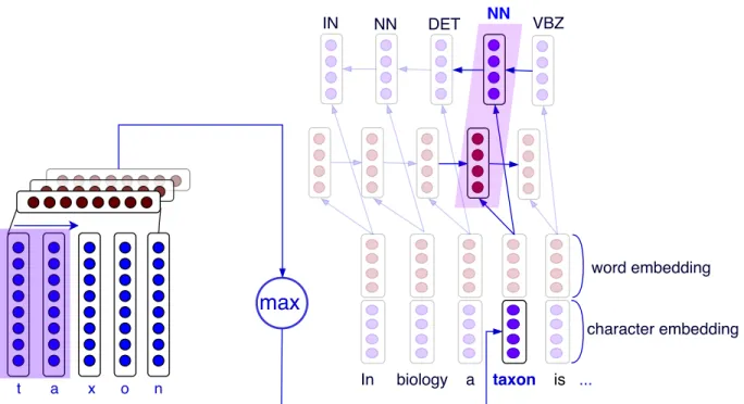
1.8 Hierarchical RNN for part-of-speech tagging with character embeddings . . . 20

1.9 Hierarchical CNN + MLP for part-of-speech tagging with character embeddings . . . 20

1.10 Hierarchical CNN + RNN for part-of-speech tagging with character embeddings . . . 21

2.1 Protein sequence splitting. . . 36

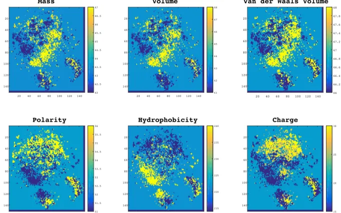
2.2 Distributions of biochemical and biophysical properties in the ProtVec-space. . . 41

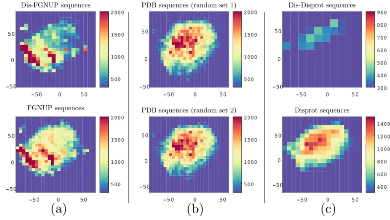
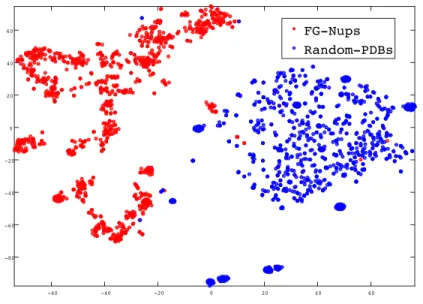
2.3 Visualization of protein sequences using ProtVec for characterization of FGNUPs . . . 44

2.4 Classification of FG-Nups versus PDB structured sequences. . . 45

2.5 The main steps of DiMotif computational workflow . . . 56

2.6 Average number of segmentation alternation in Swiss-prot . . . 57

2.7 Skip-gram neural network for training language model-based embedding. . . 62

2.8 Clustering of integrin-binding-specific motifs . . . 67

2.9 Clustering of biofilm formation-specific motifs . . . 68

2.10 Clustering of integrin-related motifs . . . 69

2.11 Different deep learning architectures implemented and evaluated in DeepPrime2Sec . . . 78

2.12 The confusion matrices of the best performing predictor for protein secondary structure prediction 82 3.1 The computational workflow of MicroPheno . . . 104

3.2 MLP Neural Networks architecture used in the host phenotype prediction in Micropheno . . . . 106

3.3 Systematic exploration of k-mer representation parameters and different classifiers . . . 108

3.4 Measuring (i) self-inconsistency and (ii) unrepresentativeness using bootstrapping . . . 108

3.5 Body-sites classification confusion matrix . . . 109

3.6 Visualization of body-sites, Crohn’s disease, and ecological environments datasets . . . 112

3.7 Computational workflow of DiTaxa . . . 121

3.8 Measuring (i) self-inconsistency and (ii) unrepresentativeness for NPEs using bootstrapping . . 125

3.9 Taxonomy of differently expressed markers for samples from patients with periodontal disease versus healthy patients. . . 128

3.10 Taxonomy of differently expressed markers for new onset rheumatoid arthritis versus healthy samples. . . 129

3.11 Taxonomy of differently expressed markers for Crohn’s disease versus healthy using DiTaxa. . . 130 3.12 Taxonomy of differently expressed markers for ulcerative colitis disease versus healthy using DiTaxa.131

(9)

3.13 Taxonomy of differently expressed markers for indeterminate colitis disease versus healthy using

DiTaxa. . . 132

3.14 Taxonomy of differently expressed markers for psoriatric disease versus healthy using DiTaxa. . 133

3.15 Taxonomy of differently expressed markers for treated rheumatoid Arthritis versus healthy samples using DiTaxa. . . 134

3.16 Heatmap of markers occurrences across samples for rheumatoid arthritis . . . 136

3.17 Heatmap of markers occurrences across samples for periodontal disease . . . 137

4.1 Clustering of 100 pivot past tense markers. . . 155

4.2 Clustering of 100 pivot present tense markers. . . 156

4.3 Clustering of 100 pivot future tense markers. . . 157

4.4 Clustering of 1000+ languages based on their tense marking using their respective top markers. 161 4.5 A map of past tense based on the largest clusters of verses with particular combinations of the past tense pivots . . . 162

4.6 A map of present tense based on the largest clusters of verses with particular combinations of the past tense pivots . . . 163

4.7 A map of future tense based on the largest clusters of verses with particular combinations of the past tense pivots . . . 164

4.8 The overview of universal adaptable sentiment lexica . . . 167

4.9 Neighbors of the word ’sensual’ in Spanish, in the bible embedding graph versus the twitter embedding graph . . . 170

4.10 Data split used in the experimental setup of UniSent evaluation . . . 172

4.11 Hierarchical clustering of fifty natural languages according to divergence of pair-wise distance distributions . . . 184

4.12 Visualization of word embedding language divergence in twelve different genomes . . . 185

5.1 The overview of the contributions of life language processing project. . . 190

5.2 Word-cloud summary of proteomics-related contributions. . . 192

5.3 Word-cloud summary of genomics/metagenomics-related contributions. . . 193

(10)

List of Tables

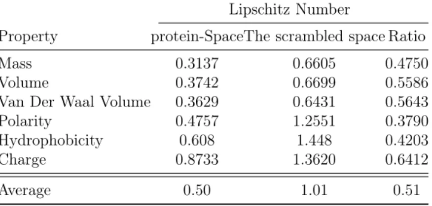
2.1 Intrinsic evaluation of the continuity of ProtVec with respect to biophysical properties . . . 42

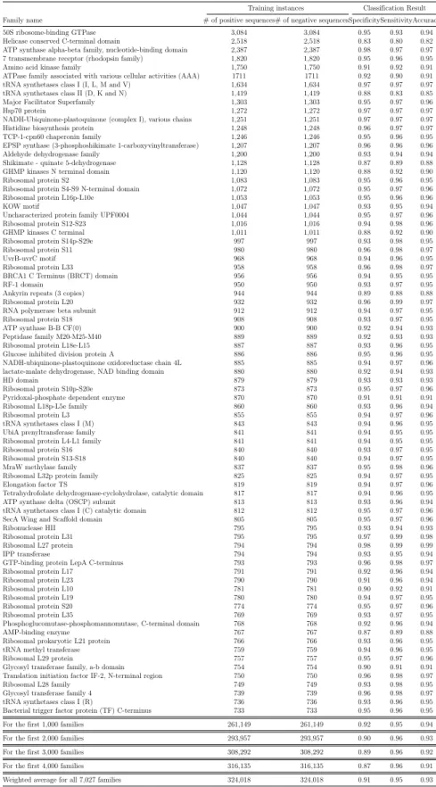
2.2 ProtVec performance in protein family classification tasks . . . 47

2.3 The performance ProtVec in FG-Nups disordered protein classification . . . 48

2.4 The accuracy of sequence labeling task in intron-exon prediction, domain identification, and secondary structure prediction . . . 48

2.5 Comparison of DiMotif, HH-Motif, and DLocalMotif . . . 63

2.6 Evaluation of DiMotif in classification of integrin-binding proteins and biofilm formation-associated proteins . . . 64

2.7 Evaluation of DiMotif in mining of NLS patterns . . . 65

2.8 Comparing k-mers, ProtVec, and ProtVecX and their combinations in protein classification . . . 70

2.9 Protein secondary structure prediction results . . . 81

2.10 Contingency table for location analysis of the misclassified amino acids . . . 82

2.11 Protein secondary structure prediction results on different deep learning architectures . . . 83

3.1 Human infection phenotype prediction cross-validation results . . . 95

3.2 Human infection phenotype prediction test set results . . . 96

3.3 Human infection phenotype prediction phylogenetic-aware-cross-validation results . . . 97

3.4 Human infection phenotype prediction phylogenetically-distant test set results . . . 98

3.5 Body-sites and Crohn’s disease prediction using k-mer representations . . . 110

3.6 Comparison of k-mer representations and OTU features in Body-sites and Crohn’s disease prediction110 3.7 The classification results for 18 ecological environments as well as 5 organismal environments . . 111

3.8 Comparison of NPEs, OTUs, and k-mer features in classification of the disease phenotype . . . 126

3.9 DiTaxa performance over synthetic dataset . . . 126

3.10 DiTaxa performance in finding the links mentioned by literature . . . 126

3.11 Comparison of a standard pipeline and DiTaxa in detecting 29 taxa with confirmed links to periodontitis . . . 135

3.12 Runtimes of DiTaxa and a common 16S processing pipeline for the periodontal, synthetic, rheumatoid arthritis and IBD datasets. . . 138

4.1 Top ten past, present, and future tense pivots extracted from 1163 languages. . . 152

4.2 MRR results for step 4. See text for details. . . 153

4.3 Language family similarity prediction results . . . 154

4.4 UniSent evaluation in Czech, German, French, Macedonian, and Spanish . . . 173

4.5 UniSent evaluation over twitter emoticon dataset . . . 173

(11)

Nomenclature

16S rRNA gene: The 16S rRNA gene is a highly conserved gene across bacteria and archaea

allowing for differential identification of taxon identities and relative abundances.

Accuracy metric Accuracy is an evaluation metric of theclassification models defined as

the number of correct predictions over the total number of predictions.

Alignment (sequence) Sequence alignment in bioinformatics refers to vertical aligning

of similar subsequences of 2 or more biological sequences (DNA, RNA, or protein) to immediately identify the similarities that are related functionally, structurally, or evolutionary.

Alignment (word) A bi-part graph relating textual units (words) of a sentence in the

source language to its translation in the target language

Amino acid Monomers of ⇡ 20 types, which are the elements for the creation of protein

polymers

Annotation Annotation in datascience refers to assigning metadata to data, which can be

done manually or automatically

Biomarker “A biomarker is a biological characteristic that is objectively measured and

evaluated as an indicator of normal biological or pathological processes or a response to a therapeutic intervention.” (Nature.com definitions)

Bootstrapping Bootstrapping refers to performing measurments using randomsampling

with replacement in statistical analysis.

Classification Classification is the process of categorizing elements according to their

observed variables. In machine learning elements are data instances, and the observed variables are datarepresentations. In biology, the elements are different organisms, the observed variables are their various characteristics in their genome or their behaviors, and the categories are the taxonomic groups.

(12)

Classifier In machine learning, classifier is a mathematical function mapping the given data points from the input representation space to the class/label representation space.

Class In machine learning, ‘class’ refers to the part of the metadata identifying the category

of a given data instance. The automatic prediction of the ‘class’ is the goal of the

classification task.

Clustering Clustering refers to the process of grouping data points according to their

observed variables. The difference between clustering and classification is that, in clus-tering, these groups are not pre-defined (clustering is unsupervised andclassif ication

is supervised).

CNN See Convolutional neural network

Convolutional Neural Network Convolutional neural network (or CNN) is a category of

deep learning models that is very common in machine learning analysis of images/videos.

A convolutional layer applies trainable convolutional functions on its input.

Convolution Convolution is a mathematical operation between two function f andg, that

can be defined as (f _⇤g)(t), R1₁f(⌧)g(t ⌧)d⌧, or in a discrete case(f _⇤g)[k] =

P1

n= 1f[n]g[k n].

Corpus A collection of written texts usually sharing some characteristics (e.g., being in a

specific language, or being from particular authors, genres, etc.)

Crohn’s disease “Crohn’s disease is a chronic inflammatory disease of the gastrointestinal

tract, mostly affecting the ileum. The inflammation can extend through the intestinal wall and tends to be asymmetric and in patches, with granulomas forming in some patients. Genetic, environmental, immunological, and bacterial factors are all thought to contribute to the disease.” (Nature.com definitions)

Dataset Dataset refers to a collection of data points usually coming together with the

metadata information in table structure.

Deep learnig Deep learning is a family of machine learning methods based on neural

networks, where the learning can be supervised, semi-supervised orsupervised.

Disordered proteins A type of, or a region in proteins lacking a fixed or ordered 3D

structure.

DisProt The dataset of disordered protein sequences

Distance In data analysis, distance refers to the mathematical measurement indicating how

far are two data points. Different data types (e.g., probabilities, real vectors, etc.) requires their proper measures of distance. Euclidean distance, KL divergence, mean squared error are instances of the defined distances between two data objects.

(13)

DNA “DNA (deoxyribonucleic acid) is the nucleic acid polymer that forms the genetic code for a cell or virus. Most DNA molecules consist of two polymers (double-stranded) of four nucleotides (A, T, C, G) that each consist of a nucleobase, the carbohydrate deoxyribose, and a phosphate group, where the carbohydrate and phosphate make up the backbone of the polymer. (Nature.com definitions)

Domain (language) domain refers to a specific language setting or context sharing a set

of meanings (e.g., sports domain or law domain).

Dropout (neural network) Dropout is a regularization method in neural network training,

which reduces the overfitting by dropping hidden units.

Embedding word embedding is a popular vector representation of words in the machine, in

a lower dimension than the vocabulary size of corpus (usually less than 1000). This representation is automatically learned using a large collection of texts and facilitates measurement of words similarities through vector similarities.

Environment Environment, in general, refers to the surroundings. In microbiology,

envi-ronments can refer to the water, soil, sediment, plant, or even animals and humans, where the bacteria can exist.

Evaluation In machine learning, evaluation refers to the process of testing the machine

learning model against expected outputs/behaviours.

F1-score F1 is a metric for theevaluationof machine learningclassif ication. F1 is defined

as a harmonic average of precision andrecall. M icro and macro averaged F1s can

be reported (see micrometrics and macrometrics)

Family A language family refers to a group of languages having a common ancestral language.

In the biology domain, similarly, a family is a taxonomic rank.

Feature In machine learning, feature refers to a measurable property or characteristic of a

data instance that is observed and can be represented as vectors or matrices for the machine.

Gene Gene refers to the functional sub-sequences of nucleotides in DNA orRNA.

Graph In mathematics, graph is an abstraction of data containing a set of vertices and edges

connecting them. The edges can be weighted or unweighted, directed or undirected

Integrin Integrins are transmembrane receptor proteins with a critical role in the cell

adhesion

k-mer In bioinformatics, k-mers are sub-sequences of length k within a biological sequence

(DNA, RNA, protein). In the language processing domain, k mers are called

(14)

KL divergence The Kullback–Leibler divergence (or shortly KL divergence) is a measure

of distance between two probability distributions.

Label In machine learning, the label usually refers to the output of classif ication, i.e., the

category of data.

Language-agnostic Independent of any specific language or prior assumption about it.

Language “a (finite or infinite) set of sentences, each finite in length and constructed out of

a finite set of elements” (Chomsky 2002)

Layer (deep learning) Adeeplearning model is usually a hierarchical model of non-linear

transformations, each of these transformations is called a layer.

Lexica A plural form of lexicon.

Lexicon Lexicon can be defined as a textualdataset, containing information about words

and their different categories.

Machine Learning Machine learning is a computer science field of study enabling the

ma-chines to make predictions/decisions without following any explicitly given instruction set. Most of machine learning approaches infer their prediction models through given examples in a mathematical or statistical framework.

Macro metrics Macro-metrics are a type ofevaluationmetrics formulti class classif ication,

which takes the unweighted average of metrics for the individual classes. Thus,

inde-pendent to the class priors, we give equal importance to all classes in the evaluation.

Marker (linguistic) A marker is an easily distinguishable text unit indicating a specific

grammatical function

Metagenome Metagenome refers to the collection of the genetic material belonging to both

the host and the microorganisms (microbiome) living at an environemnt

Micro metrics Micro-metrics are a type ofevaluationmetrics formulti class classif ication,

which takes the weighted average of metrics over allclasses. Thus,classes which are

more likely have greater influence in the evaluation.

Microbiome “The microbiome comprises all of the genetic material within a microbiota (the

entire collection of microorganisms in a specific niche, such as the human gut). This can also be referred to as the metagenome of the microbiota.” (Nature.com definitions)

Morpheme A morpheme is the smallest unit of text with meaning (dependent or

(15)

Motif P roteinshort linear motif (SLiM) sequences are short sub-sequences of usually 3 to

20 aminoacids that are presumed to have important biological functions; examples of

such patterns are cleavage sites, degradation sites, docking sites, ligand binding sites, etc.

Multi-class (classification) Multi-classclassif icationrefers to amachinelearning classif ication

setting, where the model has to choose between a set of possible categories.

n-gram Refer to the definition ofk mer.

Neural network Neural networks, or more accurately Artificial Neural Networks, are

computational models or interconnectedlayersinspired from the human neural network

to perform specific prediction tasks.

Nucleotides Nucleotides are the basic units of nucleic acids such as DNA or RNA.

OTU Operational Taxonomic Unit or shortly OTUs are clustersof similar sequence variants

of the 16SrRN A. OTUs are used to classify groups of closely related sequences.

Parallel corpus A parallel corpus is a collection of texts, where each sentence in it is

translated into one or more other languages

Periodontal disease Periodontal disease is an inflammatory disease caused by specific

microorganisms in supporting tissues of teeth.

Phenotype Phenotype refers to the observable characteristics or traits of organisms.

Pipeline Pipeline is a sequence of data processing modules, where the output of a module

is the input to the next one, and they are connected to accomplish a particular task.

Precision In a machine learning classif icationtask, precision for a class is defined as the

number of true positives divided by the total number of elements labeled as belonging to the class. M icro andmacroaveraged precisions can be reported (seemicrometrics

and macrometrics).

Primary sequence (protein) The primary sequence/structure of the protein is the linear

sequence of amino acids, which is also known as the protein sequence.

Protein Proteins are macromolecules (polymers) consisting of the chain(s) of smaller elements

(monomers) called amino acids.

Proteomics “Proteomic analysis (proteomics) refers to the systematic identification and

quantification of the complete complement of proteins (the proteome) of a biological system (cell, tissue, organ, biological fluid, or organism) at a specific point in time. Mass spectrometry is the [experimental] technique most often used for proteomic analysis.” (Nature.com definitions)

(16)

ProtVec Protein-vectors (or shortly ProtVec) are numerical representations of protein

sequences that are automatically learned. For more details please see §2.2and 2.3.

PSSM Position-Specific Scoring Matrix or shortly PSSM refers to vector size 20 representing the log-likelihood of the substitution of the 20 types of amino acids at that position in the sequence in the sequencealignment.

Random forests Random Forest (RF) is an instance ofmachinelearning classif ier

ensem-bling decision trees. In a classif icationproblem, the outcome of many simple decision

trees (the number of trees is one of the parameters of this model) are aggregated to choose the the most popular class.

Recall In amachine learning classif icationtask, recall for aclassis defined as the number

of true positives divided by the total number of elements that actually belong to the class. M icro and macro averaged recalls can be reported (see micrometrics and

macrometrics).

Recurrent Neural Network Recurrent Neural Network (RNNs) are a type of neural

networks designed for modeling and prediction over sequential data. RNNs take the

temporal relation into account by adding feedback connections allowing for conditioning on all previous time steps (for more details please see §1.2).

Reference genome Reference sequence refers to a representative set genes of a species

Representation (data) Representation refers to a form that the data on the machine is

stored and processed.

Resamples Getting samples from data with replacement.

Rheumatoid arthritis “Rheumatoid arthritis is an autoimmune disease that is

character-ized by inflammation of the joints and the subsequent destruction of cartilage and erosion of the bone. Patients with rheumatoid arthritis are treated with drugs that suppress the immune system.” (Nature.com definitions)

RNA “Ribonucleic acid (RNA) is a polymer of 4 nitrogenous bases of guanine (G), uracil (U), adenine (A), and cytosine (C) with essential roles in coding, decoding, regulation

and expression of genes.

RNN See Recurrent Neural Network

Secondary structure of proteins Protein secondary structure is a 3D pattern of the local

segments of proteins.

(17)

Semi-supervised learning Semi-supervised learning is the category of machine learning approaches considered as a transition between unsupervised learning and supervised

learning. In semi-supervised learning, we benefit from both input-output example

pairs and examples without any assigned output, where usually the second set is much larger.

Sentiment Sentiment refers to the attitude or opinion toward something. Automatic

sentiment analysis of text data is one of the crucial topics in language processing.

Sequence A chain of elements.

Sequencing (genetics) Sequencing refers to the process of determining theDN Asequence.

Sub-sequence Sub-sequence is a sequence, which is part of a longer sequence.

Subword Subword refers to parts of a word, which can be meaningful (a lemma) or without

meaning.

Supervised learning In machine learning, supervised learning refers to mapping the input

to the output (e.g., a category) based on input-output pairs of examples.

Syntax syntax refers to a set of rules governing the structure of sentences in a language.

Synthetic dataset Synthetic data refers to a type of datasets that is artificially generated,

usually for the evaluation purpose.

Taxonomy Taxonomy refers to the hierarchical grouping of organisms into categories based

on different properties, including size, shape, and gene sequences.’ (Nature.com

definitions)

Taxon A group of one or more organisms of any rank intaxonomy.

Tokenization Tokenization refers to the process of segmenting a sentence into tokens

Token A string of characters between spaces or punctuations (⇡ word).

Unsupervised learning Unupervised learning is the category of machine learning

ap-proaches drawing inference purely from the input data without having access to the metadata.

Number Sets

R Real numbers

⌦l Embedding space of language l

(18)

[• •. . .•] In figures, represents a vector representation in the neural network The element-wise product

ha,bi The inner product of vectora and b

⌦ In figures, dropout visualization in the neural network ~

x Vector x

cos(~x,~y) The cosine similarity between vectors~x, ~y

DKL(P _kQ) KL divergence between distributionsP and Q m_± Mean _± standard deviation

(19)

Acknowledgments

I would like to express my sincere thankfulness to my research advisor and dissertation chair, Professor Mohammad R.K. Mofrad, for guiding and supporting me much throughout this doctoral research. He has set an example of excellence as a mentor, researcher, instructor, and role model. It has been a great honor for me to be part of his group at Mofrad Lab, where I learned many new and interesting things. I have to thank him for being very much flexible with me in many aspects. Besides my advisor, I would like to thank Professor Shaofan Li, Professor David Bamman, and Professor Joan Bruna Estrach, my qualification exam and dissertation committee members at UC Berkeley for their great and continuous support and encouragement.

Thanks to the unique opportunity I had been given by my advisor Professor Mofrad, I had the chance to enrich my dissertation in close collaborations with the pioneers in the areas of metagenomics, as well as, natural language processing. I would like to thank Professor Alice C. McHardy, the head of the Department of Computational Biology at the Helmholtz Center for Infection Research, who co-supervised me in several research projects I carried out during my PhD. I thank her very much for her great supports, encouragements, and teachings. I was very fortunate to work with her. I have been also pleased to closely work with Professor Hinrich Schütze (the head of the center for information and language processing at the University of Munich) who co-supervised my PhD projects related to natural language processing. I deeply thank him for his supports and teachings, in many regards.

Furthermore, I thank the graduate student advisors of the AS&T program, Ariana Castro and Catalina Estrada, Berkeley International Office, and UC Berkeley Graduate Division for their exceptional care for the students.

In addition, I would like to thank my colleagues at Mofrad lab who contributed to my PhD work with their advice and supports,Kiavash Garakani,Mohammad Soheilypour,

Mohadesseh Peyro, Ruhollah Mousavi Baygi, Zeinab Jahed, Hengameh Shams,

Zainab Haydari, Mehrdad Mehrbod, and Ali Madani also the UC Berkeley students I had the opportunity to collaborate with: Andrew Dickson, Soroush Nasiriany, Kaveh Karbasi, Vikrum Nibber, Amine Mezzour, Sam Njie, and Anderson Lee. Furthermore, I thank my other mentors, friends, colleagues, and the coauthors who supported me throughout this journey from the PhD application preparation to the PhD completion in different forms, including but nor limted to:

Professor Keivan Majidzadeh,Professor Mark Finlayson, Professor Martin Vetterli,

Professor Patrick H. Winston (RIP), Professor Marianne Winslett, Professor Jean-Cedric Chappelier, Ali Vakilian, Sepideh Mahabadi, Hessameddin Akhlaghpour, Mohsen

Mahdavi-Mazdeh,Ardavan Saeedi,Saeed Mohajeri, Pedram Pad, Amin Sadeghi, Sam

Sinai, Professor Marzyeh Ghassemi, Hassan Pezeshki Modarres, Salman Faraji, Payam

Del-gosha, Nima Ahmadipour Anari, Yadollah Yaghoobzadeh, Alireza Ghasemi, Amir

(20)

Ali Sanaei, Ali Basiri, Soroush Sarabi, Amin Aghaei, Mohammad Sahrayian, Samaneh Azadi, Professor Mojtaba Azadi, Mohammad Keshavarzi, Professor M.R. Alam, Naeem Esfa-hani, Amirhossein Hashemi Astaneh, Professor Meysam Chamanzar, Professor David Searl,Meisam Ahmadi, Hamed Fathi, Elyas Heidari,Zain Zaidi, Professor Peter Bartlett, Professor Marti Hearst, Professor Ian Holmes, Professor Sandrine Dudoit, Professor N. Veld-huis, Eduardo Escobar, Professor Ali Jannesari, Arian Hosseini, Behrang Mohit, Benjamin Roth, Heike Adel, Thomas Schäfer, Alena Moiseeva, Professor Peter Rose, Peggy Hobmaier, Gary Robertson, Andreas Bremges, Philipp Münch, Tzu-Hao Kuo, Aaron Weimann, Till-Robin Lesker, Susanne Reimering, Professor Susanne Haeussler, Nina Poerner, Christoph

Ringlestetter, Fabienne Braune, Jan-Frederik Kassel, Kaya Kim, Omid Rohanian, Ali

Aghebat-Rafat, Mohammad Samavat, Ali Mollabashi, Professor Ahmad Rezaei, Motreza

Karamooz, S. Hassan Zolanvar, and Professor S. Ehsan Seyedabrishami .

I gratefully acknowledge my departmental funding sources at the University of California Berkeley in the first two years, funding resources at the University of Munich (LMU) and Helmholtz Center for Infection Research. I also thank Google for the travel award at the ICML 2016, sponsoring the best poster as well as the best paper awards at the Computational Biol-ogy and Multilingual methods workshops, respectively at ICML 2016, and NAACL-HLT 2016.

I sincerely thank my dearest parents for their unconditional love, support, and the efforts I could never compensate. You have been always very kind to me and I owe you my life. I thank my dear parents-in-law, our grandparents, Azizjoon and Mamanjoon, and my ex-tended siblings: Mahdi, Hamed, Jalal, Elaheh, Meisam, Meghdad, Ms. Mahboobeh, and Ms. Mozhdeh, and their lovely sons and daughter: Arsha, Hossein, Mahdi, Ali, Fatemeh,and Saj-jad, for their always great encouragements and forgiving us for being physically far from them.

My special thanks goes to my beloved wife, Meshkat, for her continuous support, en-couragements, and the sacrifices she made along the way. Thank you so much, Meshkat! Also, thank you for the great helps in design-related aspects of this work. With you, my life became much lighter and much more colorful!

(21)

Chapter 1 Introduction to language processing and

deep learning

1.1 Language definition and the “language of life”

Noam Chomsky introduced a broad definition for language, describing it as “a (finite or infinite) set of sentences, each finite in length and constructed out of a finite set of el-ements” (Chomsky 2002). Obviously, this definition is not limited to natural languages. An abstract representation of the internal dispositions of the macromolecules of life (i.e., nucleic acids (DNA and RNA) and proteins) satisfies this definition as well, as all of these macromolecules are polymers constructed from a finite set of smaller molecules (Cooper et al. 2000). DNA and RNA are polymers made up of sequences of nucleotides of four distinct types with the alphabetic representations {A, T, C, G_} and _{A, U, C, G_}, respectively, and

proteins are polymers made up of sequences of amino acids of 20 different types represented by alphabet characters {A, C, D, E, F, G, H, I, K, L, M, N, P, Q, R, S, T, V, W, Y}. DNA and

RNA are informational molecules, as they carry the genetic instructions needed to make proteins. In contrast to informational molecules, proteins are operational macromolecules, as they contribute to the molecular machinery that carries out the functions that are essential for life. The central dogma of molecular biology describes the relationships among DNA, RNA, and proteins along the flow of genetic information. It states that information flows from the DNA into the RNA in a process called ‘transcription’, and then further to proteins through a process called ‘translation’ (Cooper et al. 2000). Even in the terminology, the

¶_{The contents of this chapter have partially appeared in the following publications:}

1. Asgari, E., & Mofrad, M. R. (2019). Deep Genomics and Proteomics: Language Model-Based

Embedding of Biological Sequences and Their Applications in Bioinformatics. InLeveraging Biomedical

and Healthcare Data (pp. 167-181). Academic Press.

2. Adel, H. and Asgari, E. and Schütze H. (2017). Overview of Character-Based Models for Natural Language Processing. Lecture Notes in Computer Science book series (LNCS, volume 10761), 3–16.

(22)

presence of elements such as ‘transcription’ and ‘translation’ reflects the notion of viewing this information representation system as the ‘language’ of life.

Linguists and computational lin-guists consider a sentence as the out-put of a complex generative process controlled by certain rules (

Jack-endoff 1972). They distinguish

between syntactic and semantic rules. Generally, syntactic rules govern how the elements are put together to generate well-formed sentences, whereas semantic rules determine the meaning of the re-sulting sentence. Analogous to what linguists and computational linguists believe about the sequence of words in a sentence, biologists believe that protein and nucleotide (DNA and RNA) sequences are not merely one-dimensional strings of symbols. These sequences encode a lot of information about molecu-lar structure and functions in them-selves (Cooper et al. 2000). The structures and functions of

macro-molecules are interesting for us as they can provide information about genotypes, phenotypes, diseases and even treatments for diseases. Similar to the complex syntax and semantics of natural languages, certain biophysical and biochemical “grammars” dictate the formation of biological sequences. Thus it would be natural to adopt/develop methods in language processing to gain a deeper understanding of how functions and information are encoded within biological sequences, which is one of the main goals of bioinformatics (Yandell and Majoros 2002; Searls 2002; Asgari and M. R. Mofrad 2015).

Bioinformatics and natural language processing

Since this research is at the intersection of bioinformatics and natural language processing (NLP), we begin by defining these. Bioinformatics is defined as “conceptualizing biology in terms of macromolecules (in the sense of physical-chemistry) and then applying informatics techniques (derived from disciplines such as applied maths, computer science, and statistics) to understand and organize the information associated with these molecules on a large

(23)

scale” (Luscombe et al. 2001). Some of the primary data types that bioinformaticians deal with are genome sequences, macromolecular structures, the results of functional genomics, scientific literature texts, taxonomy information and interaction networks of macromolecules (Luscombe et al. 2001). Natural language processing can be defined as conceptualizing human languages in terms of written texts. Similar to bioinformatics, NLP researchers use computer science and statistical approaches to understand and manipulate texts by using machines (Chowdhury 2003), which can be very challenging because of the ambiguities that exist in natural languages (Christopher D Manning and Schuetze 1999). Bioinformatics and NLP are research areas that have greatly benefited from each other since their beginnings and there have been always methodological exchanges between them. Levenshtein distance (Levenshtein 1966) and Smith–Waterman (Waterman et al. 1976) algorithms for calculation of string or sequence distances, the use of formal languages for expressing biological sequences (Searls 1993; Searls 2002), training language model-based embeddings for biological sequences (Asgari and M. R. Mofrad 2015) and using state-of-the-art neural named entity recognition architecture (Lample et al. 2016) for secondary structure prediction (Johansen et al. 2017) are some instances of such mutual influence.

(24)

1.2 Introduction to deep learning for language

processing

The Role Representation in Language Processing

Can a computer automatically comprehend a piece of English text to find documents with similar content or automatically translate the given document to French? These types of tasks constitute the area with which Natural Language Processing (NLP) is mainly concerned. The purpose of NLP is to design algorithms allowing computers to understand natural languages for performing specific tasks (e.g., information retrieval, machine translation, and sentiment analysis). When we want to discuss a complex concept with an audience unfamiliar with the topic, we model or represent the concept within a framework that is understandable for the audience. The same logic applies in presenting a natural language text to a machine. Computers are experts in dealing with numerical values, vectors, and matrices. Thus, the first step in NLP is to vectorize natural language text for computers. Words are the conventional input units of almost all NLP tasks. Therefore, to utilize machines for language processing, we need to find proper vector representations of words that are interpretable by machines. We expect such representations to preserve some indications of similarity and dissimilarity between words. For instance, when we search a phrase in a search engine, we expect the machine to consider words ‘formula’ and ‘equation’ to be similar and consider them dissimilar to an irrelevant word like ‘cuisine’. Thus, we should attribute similar vector representations to the words ‘formula’ and ‘equation’, dissimilar to the vector representation of ‘cuisine’. As a reminder vector similarity/distance can be calculated using operations in linear algebra (e.g., dot product, Euclidian distance, and cosine similarity). Of course, semantic similarity is not the only consideration we have in NLP tasks. As an example, part-of-speech tagging is one of the routine NLP tasks, where the goal is to label words with their syntactic part-of-speech (e.g., noun, verb, adverb, etc.). Presumably, when we want to perform part-of-speech tagging, we desire a vector representation incorporating syntactic similarities.

The performance of NLP or in general any machine learning task largely depends on the quality of data representation (also known as feature extraction/engineering), to the extent that recently representation learning became an important research area in machine learning (Bengio et al. 2013; Collobert, Weston, et al. 2011). Deep neural network algorithms effectively allowed for the automatic encoding of data into a proper representation and intro-duce representation learning as a new field in itself in the realm of machine learning (Bengio et al. 2013). Recent works in the area of representation learning have proposed successful representations of data in computer vision, speech recognition, and natural language process-ing (Y. LeCun et al. 2015;Graves, Mohamed, et al. 2013;Mikolov, Sutskever, K. Chen, et al. 2013). Similar to the role of textual representations in NLP tasks, representation of biological sequences is key to many bioinformatics tasks, which is facilitated by the recent advances in deep learning (Angermueller et al. 2016).

(25)

Ono-to-one representation versus distributed representation

The most straightforward approach to represent textual units (characters, words, or sentences) for a machine is to utilize one element of computing (e.g., a cell in a vector) to represent one entity, in a way that we have a one-to-one mapping from the vector representation to the exact entities. One-to-one representation is also known as local representation. One-hot vector encoding is an instance of such a one-to-one representation. Given a set of M

words (or any other textual unit) we can represent each word wi using a vector in the size of M, where the vector has zeros everywhere except at the index of word i having the

value of 1, hence calling this representation “one-hot vector representation”. Although this representation is straightforward to obtain, it has several drawbacks: (i) this representation is not memory-efficient and not scalable when we have a large collection of textual elements, (ii) this representation does not take the similarities into account, where the similarity of vectors is defined based on their dot product or cosine similarity. In such a space of text representation all word representations of distinct words are orthogonal to each other (hwiwji= 0,i6= j and hwiwji= 1 ,i=j).

An alternative to the one-hot vector representation approach is the use of distributed representation. Distributed representations are “many-to-many”, meaning that (i) each textual unit is represented through a weighted combination of many computing elements, (ii) each computing element gets involved in the representation of many textual units (Geoffrey E Hinton 1984). For an instance manually creating such a representation, one may represent the word wi in a natural language by a vector size 2, where the first element indicates the polarity score of the word (a real value between -1 and 1) and the second element is the concreteness score of a word (a real value between -1 and 1) that are assigned by a team of experts. This way, similar words (in terms of having similar polarity and concreteness scores) would have similar representations. Distributed representations in comparison with the one-hot vector representations are much more desired for computational tasks because they are more memory efficient and can incorporate the similarities of textual units. In traditional machine learning, feature engineering played a crucial role in obtaining better performance. However, the manual designs of features/representations can be challenging, as they require domain knowledge and sufficient human resources, which are not always granted. Additionally, manually designed features are subject to be bias or incompleteness. This motivates automatic feature extraction.

Machine learning tasks can significantly benefit from the automatic learning of distributed representation. Recently, deep learning methods have achieved very high performances in many areas, including NLP, via training end-to-end models that do not require traditional task-specific feature engineerings. Next, I will provide a brief introduction to such models.

Introduction to neural networks models for language processing

Recently, neural networks models achieved state-of-the-art performance in many natural language processing tasks (Collobert, Weston, et al. 2011;Devlin et al. 2018) via end-to-end

(26)

learning eliminating traditional feature engineerings. Biological neural networks inspired the design of artificial neural networks. Almost all sorts of neural networks, in an abstract view, are multi-layered models consisting of 3 main types of layers: (i) input layer dealing with the problem domain, (ii) intermediate layer(s) mapping the problem domain to an intermediate distributed representation, and (iii) an output layer dealing with the solution domain. The intermediate layers are supposed to apply non-linear transformation(s) on the input data to prepare a proper representation before the final transformation to the target output. Finally, given the intermediate distributed representation, the output layer provides the final outputs of the model in the solution domain.

Order and Granularity: The input can be either viewed as a sequence of textual units or

as a bag (a set of items with repetition) of them. Despite the simplicity, the bag-of-words model has been proven to be very successful in many text classification tasks (Arora et al. 2016). Another consideration is the choice of the atomic unit of text in the input, which is not necessarily word and can be byte (Gillick et al. 2016), character (J. Lee et al. 2016), character n-gram (Schütze et al. 2016), byte-pairs (Sennrich et al. 2016), morpheme (Kirchhoff et al. 2006), etc.

There exist a variety of models for the intermediate layers to encode the input data; examples are convolutional layers (C. N. d. Santos and Gatti 2014), recurrent layers (Sutskever, Martens, et al. 2011), capsule network (Sabour et al. 2017;W. Zhao et al. 2018), and various combinations that different models together can make. Here, I describe the main basic models used within the framework of this dissertation.

Multi-layer preceptron neural network

Multi-Layer-Perceptrons (MLP) also known as fully-connected feedforward neural network is the basic neural architecture approximating function f⇤_{, mapping the input vector} _x_{to the}

output y through non-linear transformations parameterized with✓:

ˆ

y =f(x;✓)

The function f is called a network as this is the result of connecting multiple non-linear

layersfi’s:

f(x;✓) = fM(. . . f3(f2(f1(x)))),

where M is the number of non-linear transformations, and each fi can be parameterized as follows:

fi(xi;✓i) =gi(xiTWi+bi),

✓i ={Wi, bi}

where xi 2 RDi is the input to the ith layer and W 2 RDi⇥Di+1 is a linear transformation from the input dimensionDi to the dimension of the output of the current layer Di+1 and

(27)

function of the ith layer.

Input and output of MLP:The MLP neural network architecture is depicted in Figure 1.1.

The other name of this network is feedforward network, as the information flow is forwarded from the input xto the output y through fi’s. The MLP architecture is mainly designed for

bag-of-word input features, as the contextual and global structure of a sequence cannot be easily modeled in this architecture. However, the extended versions of MLP, i.e., convolutional and recurrent neural networks can take the sequential and global structure into account. The MLP can be used to regress real values (regression) or to predict a category (classification); the non-linear activation function of the last layer can be determined according to this objective. The gi’s are commonly chosen from the following differentiable non-linear functions:

• Sigmoid ( ): sigmoid function maps any givenx₂R to a value between 0 and 1:

gi = (x) =

1 1 +e x,

which is usually favored as the ultimate transformation in a binary classification setting. Considering a threshold of 0.5 on the out put of sigmoid it can be binarized for prediction between two classes.

• Tanh: Tangent hyperbolic function is also a non-linear function that commonly used for transfering the input x₂Rto a value between -1 and 1 and can be formulated as

follows:

gi =tanh(x) =

2

1 +e 2x 1 = 2 (2x) 1,

• Rectified linear unit (ReLU): ReLU is a very simple, but in practice a very effective

non-linear transform used in neural networks. ReLU for any given input x gives an

outputx if x is positive and 0 otherwise:

gi =ReLU(x) = max(x,0).

• Softmax: In the case of multi-class classification, the softmax activation function

is used at the last layer to produce the probability vector that can be regarded as representing posterior probabilities (Goodfellow et al. 2016).:

gi =sof tmax(xk) =

exp(xk)

⌃xl2xexp(xl)

.

Learning: Back-propagation algorithm and stochastic gradient decent

The forward propagation of information from input x to the predicted output y has been

discussed so far. Subsequently at the output layer we can measure the cost functionJ✓(y,yˆ)

based on the gold output y and the predicted output yˆ. The back-propagation algo-rithm (Rumelhart et al. 1986) allows the backward propagation of information from the cost

(28)

input layer output layer hidden layer (1) hidden layer (2) last hidden layer (M) hidden layer (M-1) W₁ 1g 2g g M -1 W2 hidden layers WM-1 Mg W_M

Figure 1.1. Architecture of Multi-Layer-Perceptrons (MLP) Neural Network with M

hidden layers and non-linear activation functions of gi’s on top of each linear transformation

using Wi matrices.

functionJ✓ calculated at the output back to the first hidden layer in the network through the

gradients over ✓1:M. Then Stochastic Gradient Descent (SGD) algorithm (Y. A. LeCun et al.

2012) is utilized to perform parameter optimization minimize the cost function using the calculated gradient in the back-propagation. This approach of learning (the combination of back-propagation and SGD) is not limited to the MLP, but applicable to any function whose derivative is defined. Different variations of SGD are proposed in the literature, including Momentum (Polyak 1964) and Adam (Kingma and Ba 2015), allowing for faster learning and more optimal parameters. To avoid overfitting, usually earlystopping and also dropout at

hidden layers (N. Srivastava et al. 2014b) are performed. Early stopping refers to stop the process of parameter optimization when further optimization only improves the performance over the training and not the test data. Dropout is a simple but powerful regularization approach for neural networks by randomly dropping out hidden units.

The loss function will be also determined based on the problem-setting. In the case of classification, the cross-entropy is the most common loss function. Given that the gold labely

presented using one-hot representation and the output layer is defined as softmax generating ˆ

y, the cost function J✓ betweeny and yˆ can be defined as follows:

J✓(y,yˆ) = ⌃i|y=1| (yilog ˆyi+ (1 yi) log (1 yˆj))

Convolutional Neural Networks (CNN)

The development of Convolutional Neural Networks has been mainly inspired by the function of human visual system containing several filters and detectors of different patterns (Fukushima 1980). Convolution operation between two given functions pand q can be defined as follows:

(p⇤q)[i] =⌃M_j₌ _Mp[i j].q[j],

where p_⇤q can be regarded as a filtered version of p by function q. Convolutional layers in

(29)

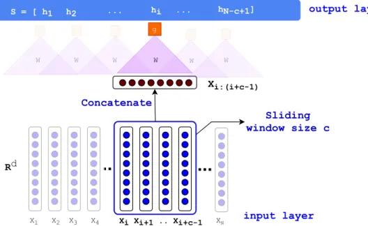
Given an input sequence of textual units (e.g., words) x0

is 2 Rd within a sentence of

length N,(N i 1), a 1D convolution of window size c, can be defined as follows (Y. Kim

2014):

hi =g(WTxi:(i+c 1) +b),

where xi:i+c 1 2Rdc represents the concatenation of xi vectors, and W 2Rdc is the

convo-lutional filter. By putting the hi’s of a sentence together (i_N c+ 1), we can generate a new representation of sentence S= [h1, h2, . . . , hN c+1]2RN c+1.

Max-pooling: a common approach for the representation of textual data after a

convolu-tional filter is applying max over timefilter to pick a value inS containing the maximum

value. The main idea is to capture the most critical activation during the time.

Rd X1 X2 X3 X4 Xi Xi+1 .. Xi+c-1 XN W X_i:(i+c-1) g hi W W S = [ h1 h2 ... ... hN-c+1] W W W Sliding window size c Concatenate output layer input layer

Figure 1.2. The architecture of Convolutional Neural Network (CNN) with a sliding

window size of c applied on a sequential data (text). The Xi (the input of CNN at time i) and c 1of its left neighbors (Xi+1, Xi+1, . . ., Xi+c 1) are concatenated to form a single

vectorXi:(i+c 1). Subsequently, Xi:(i+c 1) through a non-linear transformation

g(WT_x

i:(i+c 1)+b) produces hi (the output of CNN at time i). Next, the window is shifted to produce hi+1.

The architecture of CNN is depicted in Figure 1.2. In practice, multiple filters (multiple

W’s) are applied to the input sequence to capture multiple views from a sequence. Since

functions applied in CNN are also differentiable, the training of CNN layer is the same as learning of the MLP discussed above. The CNN layers allow for the integration of local

(30)

context in specific window sizes and stacking of CNN layers on top of each-other facilitates moving from a local context to a more global context.

Neural Sequence Modeling

Language modeling Language modeling is the task of assigning a probabilityP(w1, w2, . . . , wN)

to a given sequence of textual unit (words, phrases, or sentences) w1, w2, . . . , wN. Language modeling is a very important component in many NLP applications, in particular the appli-cations containing language generation or the evaluation of text correctness, e.g., machine translation, auto-completion of text, chat-bot, etc. Using the chain rule, this probability can be written as follows:

P(w1, w2, . . . , wN) = P(w1)⇥P(w2|w1)⇥P(w3|w1, w2)⇥. . .⇥P(wN|w1, . . . , wN 1)

For the simplicity of modeling in practice kth _{order Markov model is considered, i.e., the} _w t only depends on the k preceding textual units:

P(wt|w1, . . . , wt 1) = P(wt|wt k, . . . , wt 1),

which can be estimated by counting of n-gram of textual units, e.g., for the k = 2:

P(wt|w1, . . . , wt 1) =P(wt|wt 1, wt 1) =

count(wt 2, wt 1, wt)

count(wt 1, wt)

,

where count(wt 2, wt 1, wt)is the number of times the sequence of wt 2, wt 1, wt is observed in the whole collection of texts. In a more broad definition, w1, . . . , wt 1 is the left context of

wt. In other words, in language modeling, we study the probability ofwt given its context. By increasing the k, the model becomes more powerful in sequence modeling. However, on

the other hand, the model becomes exponentially larger, and a larger collection for estimating would be needed. Recurrent neural networks and distributed representation are alterna-tive models for the sequence modeling that can be used for the language modeling task as well.

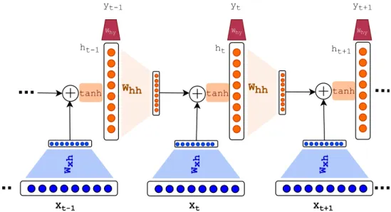
Recurrent neural network (RNN): Recurrent neural networks extend the MLP

archi-tecture for the modeling of sequential data. RNNs take the temporal relation into account by adding feedback connections allowing for conditioning on all previous states. The RNN architecture is depicted in Figure 1.3. Given the sequence input of {x1,x2, . . . ,xN}2Rdx

(e.g., sequence of words or subwords), where dx is the dimension of input text units, a single time step in the RNN can be formulated as follows:

ht=tanh(Whhht 1+xtTWxh)

ˆ

yt=sof tmax(htTWhy),

(1.1) where the ht2Rdh is the hidden state of RNN at time stept,Whh2Rdh⇥dh determines the contribution of the previous hidden state ht 1 in the current hidden state, and Wxh 2Rdx⇥dh determines the contribution of input xt in the ht. Subsequently, a transformation of ht through Why 2Rdh⇥dy as each time step produces the output yˆt. The output can be different

(31)

in different problem settings. As discussed earlier in the case of multi-class classification

sof tmax is used anddy is the number of classes we have at the output (to be comparable

with the one-hot encoding of the labels). Since in the language modeling (prediction of the next word/subword) the output is also limited to the list of vocabulary, the problem setting is the same as multi-class classification and sof tmax is used in the last layer. Please note

that the Whh, Wxh, and Why remain constant across the time steps.

Wxh X_t-1 X_t X_t+1 Whh tanh tanh tanh h_t-1 h_t h_t+1 Wxh Wxh Whh Why Why Why yt-1 yt yt+1

Figure 1.3. The architecture of Recurrent Neural Network (RNN) is shown around the

time step t. At each time step t, the Xt (the tth input element of the sequence) maps to a vector inRdh through _Wxh. Next, to produce _h

t (the hidden state at timet),xtTWxh vector is added to a transformed version of ht 1 (through Whh) and a non-linear transformation

(here tanh) is applied on top, i.e.,ht =tanh(Whhht 1+xtTWxh). ht at each step produces the output yt through a transformationWhy. Note that all W’s (Wxh, Whh, Why) are linear transformations shared across time steps.

The training process of an RNN is also similar to the MLP network, where we perform the back-propagation through time (Werbos et al. 1990). Although RNNs are supposed to take the full context of the input sequence into account, vanishing gradient (when the gradient is very small, and the weight will not be updated anymore) can occur in their training. Succeeding variants of RNNs, namely Long Short-Term Memory (LSTM) (Hochreiter and Schmidhuber 1997) and Gated Recurrent Unit (Chung, Gulcehre, et al. 2015) resolved this issue and allowed for efficient training of RNNs to incorporate long term dependencies.

Language model-based representation learning

Transfer learning in machine learning refers to the use of the solution in a problem setting (source problem) to solve a different problem (target problem). Using a neural network trained for a specific task for another task is also an instance of transfer learning. The

(32)

Xt

Xt-N Xt-N+1 Xt+N-1 Xt+N

The left context of xt The right context of xt

output layer

input layer hidden layer

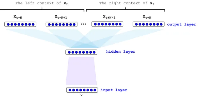
Figure 1.4. Skip-gram neural network for the training of language model-based embedding.

In this network for a given word the context words are predicted.

more general the source problem, the more target problems can benefit from the pre-trained network. Thus, an ideal scenario for a source problem would be a case with (i) enough training instances and (ii) general purpose task; then we train a proper network on the source problem and fine tune it for the target problem using a less number of training instances. This way, the pre-trained network serves as a prior knowledge from the source problem to the target problem.

Language modeling (prediction of the next word based on the given context) is an ideal task for the purpose of transfer learning because: (i) the training of a neural language model only requires the raw text without any meta-data or annotation (ii) language modeling is a very general task containing information about syntax and semantics of a language. Recently, transfer learning from the language modeling domain became very popular in NLP and successfully obtained state-of-the-art performance in many tasks. Here we describe the Skip-gram (Mikolov, Sutskever, K. Chen, et al. 2013), one of the most successful architecture to obtain the text representations, which is also used within the framework of this dissertation.

The objective of Skip-gram neural network (depicted in Figure 1.4) is analogous to the objective of the language modeling task. The difference is that the input and output are interchanged, the Skip-gram predicts the surroundings (context) for a given textual unit. Formally, the objective of skip-gram is to maximize the following log-likelihood:

M X t=1 X c2[t N,t+N] logp(wc | wt), (1.2)

where N is the surrounding window size around word wt, c is the context indices around

(33)

pairs. We parameterize this probability of observing a context word wc given wt by using word embedding: p(wc | wt;✓) = evc·vt P c0₂_Cevc0·vt , (1.3)

where C denotes all existing contexts in the training data. However, iterating over all

existing contexts is computationally expensive. This issue can be efficiently addressed by using negative sampling. In a negative sampling framework, we can rewrite Equation 1.2 as follows: T X t=1 2 4 X c2[t N,t+N] log 1 +e s(wt, wc) ₊ X wr2Nt,c log 1 +es(wt, wr) 3 5, (1.4)

where Nt,c denotes a set of randomly selected negative examples sampled from the vocabulary collection as non-contexts ofwt and s(wt, wc) =vt>·vc (parameterization with the word vector vt and the context vector vc). The sub-word level Skip-gram, known as fasttext (Bojanowski et al. 2017) improves the word representations by taking character n-grams of the sub-words into consideration in calculating the embedding of a given word. In the fasttext model, the scoring function will be based on the vector representation of n-grams (e.g., 2n6) that exist in textual units (e.g, word), s(wt, wc) = Px2Swtvx>vc.

Motivation for sub-word levels language processing in this

dissertation

Natural language processing relies on a preprocessing pipeline, such as the one described in (Gillick et al. 2016) and depicted in Figure 1.5. First, the document is tokenized. This step needs language-specific tokenization tools. The token sequence is then segmented into sentences. Afterward, the syntactic and semantic analysis is performed (usually sentence-wise). Syntactic analysis outputs part-of-speech tags, syntactic dependencies, etc. Semantic analysis extracts named entity tags, semantic roles, etc. The actual natural language process-ing/understanding (NLP/NLU) task (e.g., answering questions or extracting information) uses features from those preprocessing steps. Tokenization is a critical step in NLP that can have a great impact on the performance of the entire pipeline. Although tokenizable words in many languages seem to be an obvious choice of text processing unit, subword-level and character-level language processing has recently become popular among the NLP community to address the propagation of tokenization errors in the NLP pipeline. Since biological sequences often do not contain even naive segmentation boundaries of functional units, this problem is even more severe in bioinformatics. Thus, subword- and character-level language processing methods can be beneficial for language-agnostic processing of both natural languages and biological sequences. In section §1.3, we provide a brief survey of these new approaches organized by different task types in NLP (Adel et al. 2017).

(34)

Document token

sequence

Tokenization Segmention into

sentences POS tags, syntactic dependencies Syntactic analysis (per sentence) Semantic analysis Natural language understanding Sentences NER tags, semantic roles

Figure 1.5. Natural language preprocessing pipeline. POS, part of speech. First, the

document is tokenized. The token sequence is then segmented into sentences. Afterward, the syntactic and semantic analysis is performed (usually sentence-wise). Syntactic analysis outputs POS tags, syntactic dependencies, etc. Semantic analysis extracts named entity tags, semantic roles, etc. The actual natural language understanding (NLU) task (e.g., answering questions or extracting information) uses features from those preprocessing steps.